A multi-criteria assessment of the p-median, maximal coverage and p-center location models

ISSN 1330-3651 (Print), ISSN 1848-6339 (Online) https://doi.org/10.17559/TV-20160508131905

A MULTI-CRITERIA ASSESSMENT OF THE p-MEDIAN, MAXIMAL COVERAGE AND

p-CENTER LOCATION MODELS

Mumtaz Karatas, Nasuh Razi, Hakan Tozan

Original scientific paper Location problems consider locating facilities with the objective of finding their best locations. In most real world problems, it is common that a demand node is required to be covered with multiple facilities in order to ensure a backup supply. The backup supply is necessary especially for public or emergency service location problems where a covered demand may not be serviced if it’s designated facility is engaged serving other demands. In this study we consider three classic location models, i.e. p-median, maximal coverage and p-center, and compare their performances with respect to seven decision criteria under Q-coverage requirement. For this purpose, we generate multiple problem instances and solve each instance with the three models for different Q-values. Our numerical results reveal the pros and cons of each model to assist decision makers in determining the most promising model with respect to each assessment criteria.

Keywords: backup coverage; facility location; maximal coverage; p-center; p-median

Višekriterijska procjena modela lokacije p-srednje, maksimalne pokrivenosti i p-centralno

Izvorni znanstveni članak Problemi lokacije znače lociranje objekata s ciljem pronalaženja najbolje lokacije. Kod većine stvarnih problema uobičajeno je da zahtijevani čvor zadovoljava višestruke uvjete kako bi osigurao rezervnu opskrbu. Ta je rezervna opskrba posebno potrebna kod javnih ili problema lokacije hitne službe kada se pokrivena potražnja ne može osigurati ako je njezin za to određeni objekt zauzet pružanjem usluge drugim zahtijevima. U ovom radu razmatramo tri klasična modela lokacije, t.j. p-srednje, maksimalne pokrivenosti i p-centralno, te uspoređujemo njihovo funkcioniranje u odnosu na sedam kriterija za donošenje odluke u okviru zahtjeva Q-pokrivenosti (Q-coverage). U tu svrhu generiramo slučajeve višestrukih problema i svaki slučaj rješavamo s tri modela za različite Q vrijednosti. Naši numerički rezultati otkrivaju argumente za i protiv svakog modela koji pomažu u donošenju odluke o određivanju modela koji bi najviše odgovarao u odnosu na svaki od kriterija koji se uzimaju u obzir pri donošenju procjene.

Ključne riječi: lokacija objekta; maksimalna pokrivenost; p-centralno; p-srednje; rezervna pokrivenost 1 Introduction

Facility location problems seek the best locations for facilities such as warehouses, emergency stations, ports, fire stations or military installations. In most real life situations, the requirement of satisfying a demand with multiple facilities is essential in order to provide a backup supply. This is especially common in large scale emergency location problems where a covered (satisfied) demand may not be serviced immediately if its designated nearest facility is engaged serving other demands. In such cases one alternative would be to create a queue for the demands and serve them when their nearest facility is available. However, in emergencies, the difference between life and death can sometimes be measured in minutes. Thus a better alternative is to serve the demand with another facility with appropriate resources. This brings the necessity of developing Q-coverage location models which allow the demand to be covered by multiple facilities so that it can be served by another available facility at the time of the emergency incident. A similar concept was first introduced in [1] as backup coverage location problem. The authors define backup coverage as a situation where an extra facility can cover a demand so that the backup coverage of the node will satisfy the demand [2]. In [3], authors discuss a multiple coverage problem where each demand node must be satisfied by a number of facilities. The concept of

Q-coverage is also common in wireless sensor networks

(WSNs). In WSNs, the main purpose of providing multiple coverage is to monitor an area of interest as frequently as possible. It is also used to increase the energy efficiency of a network [4].

There exist a number of location problems and solution techniques in the literature. Research on location problems mainly focuses on three models, i.e. the p-median problems (p-MP) [5÷8], p-centre problems (p-CP) [9, 10, 11], and covering problems. Covering problems can be categorized as the set coverage problems (SCP) [12, 13, 14] and the maximal covering location problems (MCLP) [15, 16, 17]. The p-MP aims to find the locations of p facilities among n candidate locations such that the total weighted distance between all demands and their nearest facilities is minimized [18]. It arises naturally in both public and private sector for locating plants, factories, warehouses or emergency stations to serve/satisfy demand at other plants, warehouses or incident locations. The p-CP problem, aims to determine the locations of p facilities with the objective of minimizing the maximum distance of any demand to its closest facility [19]. In his work [20], Haghani states that the facility location problem mainly interests in two factors: operating cost and timeliness of response to demand. However, in some cases, decision-makers make an effort to meet maximum demand in pre-determined coverage level with limited resources. The maximal covering location problem (MCLP) seeks to maximize the total number of demands supplied with a given number of facilities and designated budget [17, 21].

Although there is a rich stream of literature on these classic facility location models, there is no study that evaluates and compares the performances of the models under Q-coverage requirement with respect to multiple criteria. In this study, our main ambition is to compare the classic p-MP, MCLP and p-CP location models with respect to multiple performance criteria that are

specifically designed to reveal the strong and weak sides of each model when multiple coverage, i.e. backup coverage, for each demand node is required. For this purpose, we first generate several problem instances by creating demand and candidate facility locations random uniformly in a square region. Next, we solve each instance by all the three location models for different coverage requirement and coverage range. Finally, we analyse the performance of each location model with respect to the seven performance criteria and discuss their strong and weak sides for each problem setting.

The paper is organized as follows: a literature research of location models is presented in Section 2. We explain the formulation of Q-coverage location models in Section 3. Section 4 includes the numerical results. Sections 5 and 6 include a discussion and conclusion of our work, respectively.

2 Literature Review

There are a number of p-MP model applications in literature considering interesting location problems. In their study [22], authors utilize p-MP Mixed Integer Program (MIP) model to determine sensor locations in municipal water networks with the aim of minimizing impact of contamination in municipal water. They use the analytic model to react rapidly in case of emergencies such as accidental contamination or chemical terrorist attacks on municipal water networks, which are threatening cases on the public health. In [23], Antunes formulates a combined optimization model of p-MP and capacitated-facility-location models to deal with the problem of determining solid-waste facility locations in Central Portugal. The problems associated with allocating large-scale emergency response systems is also a common application field of p-MP models. For example, in their study [24], Serra and Marianov develop a p-MP model to allocate fire stations in Barcelona. In another study [25], authors evaluate the efficiency of p-MP approach with others, such as covering and center models, on Large-scale Emergency Medical Service (LEMS) in the Los Angeles area. In [26], an optimization model with p-MP is prepared to allocate SAR helicopters with the aim of intercept maritime incidents rapidly.

In [27] the authors utilize p-MP and p-CP models in order to seek the locations of security teams to maintain security for United States Air Force (USAF) Intercontinental Ballistic Missile Systems. Their model minimizes both the distances travelled and the maximum distance from any missile site to required security forces. First defined in [15], researchers applied the MCLP to various facility location sectors such as allocation of security-military firms, warehouses, emergency systems and healthcare facilities. In their study [28], authors formulate a MCLP model for determining the locations of video sensors to control the security of an urban area. In another military application, [29] study the problem of enhancing maintenance schedules of Intercontinental Ballistic Missiles (ICBM) for a given security requirement level. They formulate a two-stage MCLP model with the objective of maximizing the satisfaction level of demands at missile alert facilities while

systems and healthcare facilities, it is important to develop a location plan which allows serving maximum number of people with limited resources on hand. In [30], researchers study the problem of determining the locations for delivering medicines in a large city under a possible bio-terror attack. They develop a special case of the MCLP which considers the distance-dependent coverage and demand uncertainty and apply the model to a possible anthrax attack scenario in the city of Los Angeles. In a similar study [31], a Capacitated MCLP model is utilized to allocate the healthcare facilities in Selangor, Malaysia. As a solution approach, they propose a genetic algorithm which analyses the ratio of coverage of the emergency facilities within the allowable distance specified. In another study [32], the researchers develop a multi-objective MCLP formulation with the objective of locating the regional assets to respond to large-scale emergencies. Ref. [33] discusses and reviews the use of MCLP model for the maximum covering species problem. In a number of facility location problems, decision makers require covering each demand point for more than one facility at any time. Thus, the problem becomes a

Q-coverage (also known as K-coverage) problem in

which the objective is to cover each demand point in the area of interest with at least Q facilities. WSN problems constitute a large amount of Q-coverage applications in literature. Chaudhary and Pujari study the problem with the objective of maximizing sensor network lifetime while satisfying the desired Q-coverage level and propose a heuristic algorithm which provides approximate solutions to optimal [34]. In their study [35], authors consider three kinds of sensor deployment patterns, such as square unit grids deployment, random uniform deployment and Poisson deployment of n sensors while retaining Q-coverage level of protected area at all times. In addition, they consider the sleep schedule of sensors in order to extend the lifetime of the WSN. In another study [36], Hefeeda and Bagheri aim to deploy a WSN for early detection of forest fires in British Columbia, Canada and formulate the problem as a node Q-coverage problem. In [37] Curtin, Hayslett-McCall, and Qiu develop a methodology to integrate Geographic Information System (GIS) with linear programming optimization for generating alternative optimal solutions. They also study the problem of locating police patrol and account for the backup coverage.

Classic facility location problems have been modified to interest in multiple facility types and multiple coverage. In [38], Daskin and Stern formulate Hierarchical Objective Set Covering (HOSC) to determine minimum number of emergency medical service (EMS) vehicles for covering all demand locations while maximizing the extent of multi-covered zones. In [39], authors formulate a model to deploy ambulances in Santa Domingo, Dominican Republic. They aim to maximize the multiple coverage of demands within a pre-determined critical response time with limited number of vehicles. In [40], McLay develops the maximum expected coverage location problem with two types of servers (MEXCLP2) to consider multiple server/facility and demand types and improves survival rates achieved in previous EMS models. In addition to these approaches

excellent vision to covering problems in facility location. For example, [41] reviews the classic median, center and covering models. Another distinguished review [2] categorizes covering problems and presented all aspects of each sub-categorize neatly. In [42], authors survey classical facility locations problems and develop a general facility location model which can be shaped as median, center and covering model. They apply the model as covering, center and median models for allocating medical supply storage to distribute antibiotics, vaccines and drugs rapidly under a possible chemical, biological, radiological and nuclear (CBRN) terrorist attack in the city of Los Angeles and compare those models.

3 Location model formulations

Different from the classical facility location problems, in this study we consider the Q-coverage problem with primary and backup facility assignments and compare the location models with respect to seven criteria. For each demand, we name its nearest facility as the primary facility. In cases when multiple coverage (Q>1) is required, all non-primary facilities that are assigned to a demand are named as the backup facilities. Since the coverage range is not considered in p-MP and

p-CP models, for those location models we provide Q-coverage to a demand by assigning it with one primary

and Q-1 backup facilities regardless of their distance to the demand.

3.1 Q-coverage p-MP problem formulation 3.1.1 Sets and Indices

i I∈ : set of candidate locations

j J∈ : set of demand locations 3.1.2 Parameters

m = number of candidate sites (m = |I|) p = number of candidate facilities n = number of demand locations (n = |J|) hj = weight of demand j

dij = distance between locations i and j

Q = minimum number of coverage (assignment)

required

3.1.3 Decision variables

1, demand is assigned to a facility at location 0, otherwise

ij j i

x =  

1, a facility is sited at location 0, otherwise i i y =   3.1.4 Objective function min _{j ij ij} i I j J h d x ∈ ∈

∑∑

(1) 3.1.5 Constraints i i I y p ∈ =

∑

(2) , ij i I x Q j J ∈ = ∀ ∈

∑

(3) , , ij i x ≤y ∀ ∈i I j J∈ (4)

{ }

, 0,1 , , i ij y x ∈ ∀ ∈i I j J∈ (5) The objective function (1) seeks to minimize the total weighted distance between demands and their nearest facilities. Constraint (2) restricts the number of sited facilities to p. Constraint (3) ensures that all demand locations are covered by Q facilities. Constraint (4) ensures that the facilities that are not activated cannot cover any demand. Constraint (5) declares the variable types.

3.2 Q-coverage MCLP problem formulation

In addition to the notation defined above, for formulating the MCLP problem we define the additional set Nj = ∈

{

i I dij ≤r

}

where r is the maximum range of

a facility. We also define the xj variable as follows:

1, demand is assigned to a facility 0, otherwise j j x =   3.2.1 Objective function max j j j J h x ∈

∑

(6) 3.2.2 Constraints i i I y p ∈ =

∑

(7) , i j i N j y x Q j J ∈ ≥ ∀ ∈

∑

(8)

{ }

, 0,1 , , i j y x ∈ ∀ ∈i I j J∈ (9) The objective function (6) aims to maximize the total weighted number of demands covered. Constraint (7) restricts the number of sited facilities to p. Constraint (8) ensures that all demand locations are covered by at least

Q facilities. Constraint (9) declares the variable types.

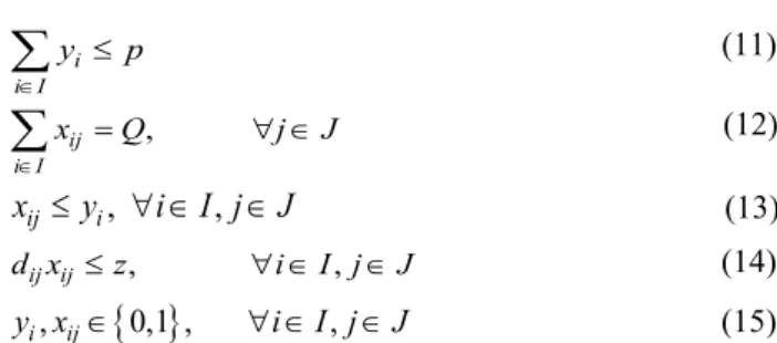
3.3 Q-coverage p-Center problem formulation

The p-CP model aims to minimize the maximum distance between demand nodes and facilities. For this reason, the p-CP model is also known as the minimax model.

3.3.1 Objective function

3.3.2 Constraints i i I y p ∈ ≤

∑

(11) , ij i I x Q j J ∈ = ∀ ∈

∑

(12) , , ij i x ≤ y ∀ ∈i I j J∈ (13) , , ij ij d x ≤z ∀ ∈i I j J∈ (14)

{ }

, 0,1 , , i ij y x ∈ ∀ ∈i I j J∈ (15) The objective function (10) seeks to minimize the maximum distance between demands and their nearest facilities. Constraint (11) restricts the number of sited facilities to p. Constraint (12) ensures that all demand locations are covered by Q facilities. Constraint (13) ensures that the facilities that are nor activated cannot cover any demand. Constraint (14) assigns the maximum distance to the objective function value. Finally, Constraint (15) declares the variable types.

3.4 Performance Criteria

This section introduces the criteria used to compare the performances of three location models. The criteria considered in this study aim to measure and examine the efficiency of the solutions basically in terms of mean distances between demand locations and facilities, number of demand covered and maximum distance between demand locations and facilities. In specific we define seven performance criteria as follows:

• C1 - Mean distance to primary: This criterion

evaluates the mean distance between each demand location and its nearest facility. Being a very common criterion, especially in emergency service location analysis studies, this performance metric aims to measure the effectiveness of a given solution in terms of average travel distance. If the problem incorporates mobile demands or facilities with different speeds (such as ambulances or search and rescue vehicles) another alternative to measure of proximity would be the mean response time instead of distance. For the MCLPand p-CP models, we assign each demand with a primary facility without considering the maximum range of a facility. • C2 - Mean distance to primary and backup: This

criterion evaluates the mean distance between each demand and its all designated Q facilities. In other words, this criterion measures the performance of a solution considering the distances to both primary and backup coverage locations.

• C3 - Mean distance to backup(s): This criterion

evaluates the mean distance between each demand and its designated Q-1 backup facilities. The main purpose of this criterion is to measure the effectiveness of backup supplies when the primary is busy with serving other demands. A short mean distance to the backup facilities plays an important role to enhance the performance of an allocation plan especially in cases where the amount of demand is high.

• C4 - Ratio of demand with both primary and backup

coverage within a range threshold: This criterion

by at least Q facilities. To make a fair comparison, when measuring the performance of the p-MP and p-CP models, we compute this value by implementing the coverage range r to each facility as utilized in the MCLP model. This ratio expresses the ratio of demands that can receive both primary and backup service within a certain time.

• C5 - Ratio of demand with at least primary coverage

within a range threshold: This metric quantifies the ratio of demand locations that are covered by at least one facility. Once again we utilize the r parameter for measuring the performance of the p-MP and p-CP models. By computing this ratio we seek to determine the ratio of demands that receive at least one service within a time or distance threshold.

• C6 - Maximum distance to primary: In this criterion

we aim to determine the worst case performance of a location model by computing the maximum distance between a demand and its primary facility.

• C7 - Maximum distance to backup(s): Similar to C6,

this criterion determines the maximum distance between a demand and its backup facilities.

4 Numerical Results

In our numerical trials, we generate demand and candidate facility locations uniform randomly inside a 100 × 100 km square region. We fix the basic parameters as m=20, n=200 and p=10. For all trials we assume that demands are of equal weight of 1. For each problem setting we perform 30 replications and solve each replication with all location models for r = 10, 15, 20, 25, 30, 35 and 40 km and for each Q = 1, 2 and 3. Fig. 1 shows the primary and backup facility assignments for an exemplary problem instance. In Fig. 1(a) each demand is assigned to its nearest facility (primary only) since Q = 1. In Figs. 1(b) and 1(c) each demand is additionally assigned to one and two backup facilities, respectively.

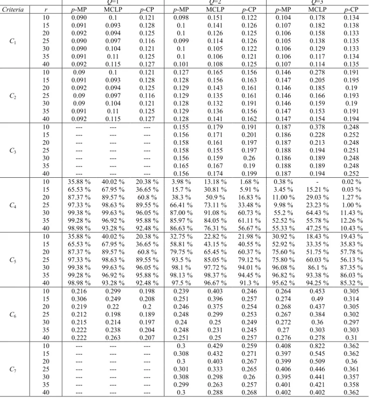
We generate problem instances and solve the optimization models in the General Algebraic Modeling System (GAMS©) environment using CPLEX 12.2.0.2. Tab. 1 summarizes the performances of models with respect to all criteria for each r value. The values for C1,

C2, C3, C6 and C7 in the table are normalized by dividing

each of them with the maximum distance possible in the area, 100 2 . The values in the tables represent the averaged values over all 30 replications. We use those averaged values to compare the models considered in this study.

Numerical results reveal the strong and weak sides of location models in terms of seven performance criteria. Figures 2 to 6 (see Appendix A) show the results for each criteria except C2 and C3. In particular;

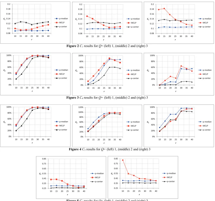
• For C1: p-MP outperforms MCLP and p-CP for all

values of Q and r. However, although MCLP outperforms

p-CP when Q=1, for Q>1 MCLP ends up with shorter

mean distances to primary facilities when r is large. • For C2: similar to C1, p-MP outperforms MCLP and

p-CP for all values of Q and r. In this case, for Q>1

MCLP outperforms p-CP when r is small (r=15 and 20). • For C3: since there is no backup assignment for Q=1,

p-MP almost outperforms MCLP and p-CP for all values

of Q>1 and r. When Q=2, p-CP performs worst, but for

Q=3, p-CP performs better than MCLP for only r=10.

• For C4: In this criterion MCLP outperforms other

models for all Q and r, except in the case where p-MP performs better for the maximum value of r. In all cases,

p-CP is the worst location model.

• For C5: p-MP outperforms other two models for all Q

values. For the case where r is large, MCLP performs best.

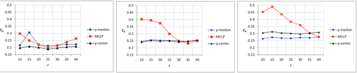
• For C6: When Q=1, p-CP outperforms the other

models for all values of r. When Q=2, p-MP and p-CP perform almost the same and the difference with MCLP gets smaller as r increases. Furthermore, MCLP outperforms p-MP and p-CP for r>30. The characteristic of MCLP is the same for Q=3, however p-MP performs significantly better than p-CP for all r.

• For C7: since there is no backup assignment for Q=1,

this data is only available for Q>1. In all cases p-CP outperforms MCLP and p-MP. The performance of MCLP gets better as r increases.

Table 1 Experimental results

Q=1 Q=2 Q=3 Criteria r p-MP MCLP p-CP p-MP MCLP p-CP p-MP MCLP p-CP C1 10 0.090 0.1 0.121 0.098 0.151 0.122 0.104 0.178 0.134 15 0.091 0.093 0.128 0.1 0.141 0.126 0.107 0.182 0.138 20 0.092 0.094 0.125 0.1 0.126 0.125 0.106 0.158 0.133 25 0.090 0.097 0.116 0.099 0.114 0.126 0.105 0.138 0.135 30 0.090 0.104 0.121 0.1 0.105 0.122 0.106 0.129 0.133 35 0.091 0.11 0.125 0.1 0.106 0.121 0.106 0.117 0.134 40 0.092 0.115 0.127 0.101 0.108 0.125 0.107 0.114 0.135 C2 10 0.09 0.1 0.121 0.127 0.165 0.156 0.146 0.278 0.191 15 0.091 0.093 0.128 0.128 0.156 0.163 0.147 0.205 0.195 20 0.092 0.094 0.125 0.129 0.143 0.161 0.146 0.185 0.19 25 0.09 0.097 0.116 0.129 0.135 0.161 0.146 0.166 0.193 30 0.09 0.104 0.121 0.128 0.132 0.191 0.146 0.159 0.19 35 0.091 0.11 0.125 0.129 0.136 0.156 0.147 0.153 0.191 40 0.092 0.115 0.127 0.128 0.141 0.162 0.147 0.154 0.194 C3 10 --- --- --- 0.155 0.179 0.191 0.187 0.378 0.248 15 --- --- --- 0.156 0.171 0.201 0.186 0.228 0.252 20 --- --- --- 0.158 0.161 0.197 0.187 0.213 0.248 25 --- --- --- 0.158 0.155 0.197 0.188 0.194 0.251 30 --- --- --- 0.156 0.159 0.26 0.186 0.189 0.248 35 --- --- --- 0.165 0.167 0.19 0.188 0.189 0.248 40 --- --- --- 0.156 0.174 0.199 0.187 0.194 0.252 C4 10 35.88 % 40.02 % 20.38 % 3.98 % 13.18 % 1.68 % 0.38 % - 0.02 % 15 65.53 % 67.95 % 36.65 % 15.7 % 30.81 % 5.91 % 3.45 % 15.21 % 0.03 % 20 87.37 % 89.57 % 60.8 % 38.3 % 50.9 % 16.83 % 11.00 % 29.03 % 1.27 % 25 97.33 % 98.63 % 89.55 % 66.41 % 73.11 % 33.48 % 9.98 % 23.23 % 1.00 % 30 99.38 % 99.63 % 96.05 % 87.00 % 91.08 % 60.73 % 55.2 % 64.43 % 11.43 % 35 99.28 % 96.92 % 95.88 % 85.97 % 84.05 % 61.11 % 52.52 % 55.78 % 12.26 % 40 98.98 % 93.28 % 92.48 % 86.63 % 76.31 % 56.67 % 55.33 % 47.25 % 10.43 % C5 10 35.88 % 40.02 % 20.38 % 32.75 % 22.82 % 21.98 % 30.92 % 18.43 % 19.43 % 15 65.53 % 67.95 % 36.65 % 58.81 % 43.15 % 40.55 % 52.92 % 33.35 % 35.83 % 20 87.37 % 89.57 % 60.8 % 79.75 % 65.45 % 60.37 % 75.60 % 51.75 % 57.78 % 25 97.33 % 98.63 % 89.55 % 93.5 % 85.05 % 79.12 % 75.80 % 60.03 % 56.13 % 30 99.38 % 99.63 % 96.05 % 98.1 % 97.72 % 94.01 % 96.08 % 86.1 % 87.35 % 35 99.28 % 96.92 % 95.88 % 98.13 % 98.37 % 94.45 % 96.82 % 93.38 % 86.03 % 40 98.98 % 93.28 % 92.48 % 97.5 % 96.67 % 91.3 % 95.62 % 94.25 % 85.32 % C6 10 0.216 0.299 0.198 0.239 0.403 0.246 0.264 0.453 0.305 15 0.306 0.249 0.208 0.251 0.396 0.257 0.274 0.49 0.314 20 0.219 0.22 0.2 0.246 0.375 0.254 0.268 0.437 0.305 25 0.212 0.198 0.189 0.248 0.299 0.253 0.267 0.384 0.302 30 0.215 0.214 0.197 0.24 0.25 0.249 0.272 0.36 0.297 35 0.222 0.238 0.204 0.248 0.231 0.245 0.27 0.303 0.303 40 0.222 0.263 0.207 0.251 0.25 0.257 0.276 0.278 0.31 C7 10 --- --- --- 0.3 0.429 0.259 0.408 0.822 0.362 15 --- --- --- 0.308 0.432 0.271 0.397 0.545 0.362 20 --- --- --- 0.3 0.403 0.267 0.399 0.509 0.36 25 --- --- --- 0.301 0.333 0.265 0.406 0.446 0.361 30 --- --- --- 0.308 0.298 0.26 0.395 0.441 0.357 35 --- --- --- 0.299 0.263 0.257 0.401 0.421 0.358 40 --- --- --- 0.3 0.288 0.268 0.402 0.402 0.362

Figure 1 Example of primary and backup facility assignments for (a) Q = 1; (b) Q = 2; (c) Q = 3. Each line represents the assignment for a demand. For

Q = 2 and Q = 3 each demand is assigned with both primary and backup facilities. Blue solid, green dashed and purple dotted lines represent the assigned primary, first backup and second backup facilities, respectively.

Figure 2 C1 results for Q= (left) 1, (middle) 2 and (right) 3

Figure 3 C4 results for Q= (left) 1, (middle) 2 and (right) 3

Figure 4 C5 results for Q= (left) 1, (middle) 2 and (right) 3

Figure 5 C6 results for Q= (left) 1, (middle) 2 and (right) 3 In general, for all values of r, p-MP outperforms

MCLP and p-CP in terms of mean distance to primary, mean distance to primary and backup, and mean distance to backup(s), as expected. The average difference for all r

between p-MP and MCLP increases as the required coverage is increased. On the average p-MP outperforms MCLP in C1 by 4 % for Q=1, 36 % for Q=2 and 49 % for

Q=3. Considering C, p-MP outperforms MCLP 0 20 40 60 80 100 0 10 20 30 40 50 60 70 80 90 100 (a) Q=1 0 20 40 60 80 100 0 10 20 30 40 50 60 70 80 90 100 (b) Q=2 0 20 40 60 80 100 0 10 20 30 40 50 60 70 80 90 100 (c) Q=3 0.08 0.1 0.12 0.14 0.16 0.18 0.2 10 15 20 25 30 35 40 C1 r p-median MCLP p-center 0.08 0.1 0.12 0.14 0.16 0.18 0.2 10 15 20 25 30 35 40 C1 r p-median MCLP p-center 0.08 0.1 0.12 0.14 0.16 0.18 0.2 10 15 20 25 30 35 40 C1 r p-median MCLP p-center 0% 20% 40% 60% 80% 100% 10 15 20 25 30 35 40 C4 r p-median MCLP p-center 0% 20% 40% 60% 80% 100% 10 15 20 25 30 35 40 C4 r p-median MCLP p-center 0% 20% 40% 60% 80% 100% 10 15 20 25 30 35 40 C4 r p-median MCLP p-center 0% 20% 40% 60% 80% 100% 10 15 20 25 30 35 40 C5 r p-median MCLP p-center 0% 20% 40% 60% 80% 100% 120% 10 15 20 25 30 35 40 C5 r p-median MCLP p-center 0% 20% 40% 60% 80% 100% 10 15 20 25 30 35 40 C5 r p-median MCLP p-center 0.25 0.35 0.45 0.55 0.65 0.75 0.85 10 15 20 25 30 35 40 C7 r p-median MCLP p-center 0.25 0.35 0.45 0.55 0.65 0.75 0.85 10 15 20 25 30 35 40 C7 r p-median MCLP p-center

approximately by 4 % for Q=1, 20 % for Q=2 and 24 % for Q=3. Lastly the difference in C3 is approximately 10

% for Q=2 and 17 % for Q=3. MCLP outperforms p-MP and p-CP only in terms of the ratio of demand with both primary and backup coverage (C4) within the range

threshold. This is mainly because the purpose of MCLP is solely to maximize the number of demands with Q-coverage. As expected both models perform better for large values of r.

Figure 6 C7 results for Q= (left) 2 and (right) 3 5 Discussion

Among the seven criteria, the first group: C1, C2 and

C3 aim to measure the performance of the models in terms

of mean distance to their assigned facilities, the second group: C4 and C5 measure the ratio of demands within a

certain range threshold, and the third group: C6 and C7

aim to measure to worst case performances by determining the maximum distance of a demand to its assigned facility. Hence, one would attempt to adopt

p-MP to satisfy first group of criteria, MCLP for the

second group, and p-CP in the third group. However, our numerical results revealed some interesting facts and showed that the perceived selection strategies do not always perform as good as expected.

Table 2 Best location models with respect to each criterion.

Q=1 Q=2 Q=3

r small large small large small large

C1 p-MP p-MP p-MP p-MP p-MP p-MP C2 p-MP p-MP p-MP p-MP p-MP p-MP C3 --- --- p-MP p-MP p-MP p-MP C4 MCLP p-MP MCLP p-MP MCLP p-MP C5 MCLP p-MP p-MP p-MP p-MP p-MP C6 p-CP p-CP p-MP MCLP p-MP p-MP C7 --- --- p-CP p-CP p-CP p-CP

Tab. 2 represents the best location models with respect to each criterion, Q value and r range. In general

p-MP is the most effective model that can be used to

maximally satisfy the criteria C1, C2, C3 and C5. Although,

based on its definition, MCLP seems to have an advantage for criteria C4 and C5, it only outperforms other

for small r in C4. On the other hand, p-CP is only

suggested in problems where the main objective is to minimize the maximum distance to only the primary when Q=1, and to the backups for Q>1. Interestingly

p-MP and in some cases MCLP outperforms p-CP in the

third group. 6 Conclusion

In this study we evaluated the performances of three classic facility location problems, i.e. p-MP, MCLP and

p-CP, under Q-coverage requirement with respect to

seven performance criteria. Our methodology involves generating multiple scenarios and solving each scenario

by three location models for different Q and r values. In order to create a fair comparison of models, we evaluated them for three groups of criteria; mean distances to primary and/or backup coverages, ratio of demand with primary and/or backup coverage, and maximum distance to primary/backup coverages. The results reveal some interesting facts on the suggested use of each location model. In general, p-MP outperforms other models in four criteria out of seven. MCLP is only preferred when the decision maker wants to maximize the ratio of demand with both primary and backup coverage when the range threshold r is small. For higher ranges, p-MP is the best option. And, for Q>1, p-CP is not the best option even though the decision maker seeks to minimize the maximum distance to primary. Thus, a decision maker who wants to minimize the mean distance to designated facilities while trying to maximize the ratio of demand locations with at least a primary coverage should prefer p-MP to MCLP.

We believe that this study is novel in the sense that it is the only study which compares the classic facility location models with respect to multiple criteria and Q-coverage requirement. Future work may consider the sensitivity of our comparison results to changes in other factors, such as the number of demands and facilities, and the size of the area. Future work may also extend the comparison for other extensions of the models, such as capacitated facilities, stochastic demand, etc.

Acknowledgements

An earlier version of this paper was presented at the International Conference on Manufacturing Engineering and Materials (ICMEM 2016), Nový Smokovec, Slovakia.

7 References

[1] Hogan, K.; ReVelle, C. Concepts and applications of backup coverage. // Management Science. 32, 11(1986), pp. 1434-1444. https://doi.org/10.1287/mnsc.32.11.1434

[2] Farahani, R. Z.; Asgari, N.; Heidari, N.; Hosseininia, M.;Goh, M. Covering problems in facility location: A review. // Computers & Industrial Engineering. 62, 1(2012), pp. 368-407. https://doi.org/10.1016/j.cie.2011.08.020

[3] Kolen, A.; Tamir, A. Discrete location theory. Wiley-Interscience, New York, 1990.

0.15 0.2 0.25 0.3 0.35 0.4 0.45 0.5 10 15 20 25 30 35 40 C6 r p-median MCLP p-center 0.15 0.2 0.25 0.3 0.35 0.4 0.45 0.5 10 15 20 25 30 35 40 C6 r p-median MCLP p-center 0.15 0.2 0.25 0.3 0.35 0.4 0.45 0.5 10 15 20 25 30 35 40 C6 r p-median MCLP p-center

[4] Zoë, A.; Goel, A.; Plotkin, S. Set k-cover algorithms for energy efficient monitoring in wireless sensor networks. // Proceedings of the 3rd International Symposium on Information Processing in Sensor Networks / Berkeley CA, 2004, pp. 424-432.

[5] Hakimi, S. L. Optimum locations of switching centers and the absolute centers and medians of a graph. // Operations Research. 12, 3(1964), pp. 450-459.

https://doi.org/10.1287/opre.12.3.450

[6] Church, R. L.; ReVelle, C. S. Theoretical and Computational Links between the p-Median, Location Set-covering, and the Maximal Covering Location Problem. // Geographical Analysis. 8, 4(1976), pp. 406-415.

https://doi.org/10.1111/j.1538-4632.1976.tb00547.x

[7] Campbell, J. F. Hub location and the p-hub median problem. // Operations Research. 44, 6(1996), pp. 923-935. https://doi.org/10.1287/opre.44.6.923

[8] Church, R. L.; Scaparra, M. P.; Middleton, R. S. Identifying critical infrastructure: the median and covering facility interdiction problems. // Annals of the Association of American Geographers. 94, 3(2004), pp. 491-502.

https://doi.org/10.1111/j.1467-8306.2004.00410.x

[9] Drezner, Z. The planar two-center and two-median problems. // Transportation Science. 18, 4(1984), pp. 351-361. https://doi.org/10.1287/trsc.18.4.351

[10] Suzuki, A.; Drezner, Z. The p-center location problem in an area. // Location science. 4, 1(1996), pp. 69-82.

https://doi.org/10.1016/S0966-8349(96)00012-5

[11] Davidović, T.; Ramljak, D.; Šelmić, M.; Teodorović, D. Bee colony optimization for the p-center problem. // Computers & Operations Research. 38, 10(2011), pp. 1367-1376. https://doi.org/10.1016/j.cor.2010.12.002

[12] Beasley, J. E.; Jörnsten, K. Enhancing an algorithm for set covering problems. // European Journal of Operational Research. 58, 2(1992), pp. 293-300.

https://doi.org/10.1016/0377-2217(92)90215-U

[13] Badri, M. A.; Mortagy, A. K.; Alsayed, C. A. A multi-objective model for locating fire stations. // European Journal of Operational Research. 110, 2(1998), pp. 243-260. https://doi.org/10.1016/S0377-2217(97)00247-6

[14] Caprara, A.; Toth, P.; Fischetti, M. Algorithms for the set covering problem. // Annals of Operations Research. 98, 1-4(2000), pp. 353-371.

[15] Church, R.; ReVelle, C. The maximal covering location problem. // Papers in Regional Science. 32, 1(1974), pp. 101-118. https://doi.org/10.1007/BF01942293

[16] Schilling, D. A.; Jayaraman, V.; Barkhi, R. A Review of Covering Problems In Facility Location. // Computers & Operations Research.1, 1(1993), pp. 25-55.

[17] Balcik, B.; Beamon, B. M. Facility location in humanitarian relief. // International Journal of Logistics. 11, 2(2008), pp. 101-121. https://doi.org/10.1080/13675560701561789

[18] Tansel, B. C.; Francis, R. L.; Lowe, T. J. State of the art— location on networks: a survey. Part I: the center and p-median problems. // Management Science. 29, 4(1983), pp. 482-497. https://doi.org/10.1287/mnsc.29.4.482

[19] Razi, N.; Karatas, M. A multi-objective model for locating search and rescue boats. // European Journal of Operational Research. 254, 1(2016), pp. 279-293.

https://doi.org/10.1016/j.ejor.2016.03.026

[20] Haghani, A. Capacitated maximum covering location models: Formulations and solution procedures. // Journal of Advanced Transportation. 30, 3(1996), pp. 101-136. https://doi.org/10.1002/atr.5670300308

[21] Karatas, M.; Razi, N.; Tozan, H. A Comparison of p-median and Maximal Coverage Location Models with Q– coverage Requirement. // Procedia Engineering, 149, (2016), pp. 169-176.

https://doi.org/10.1016/j.proeng.2016.06.652

[22] Berry, J.; Hart, W. E.; Phillips, C. A.; Uber, J. G.; Watson, J. P. Sensor placement in municipal water networks with temporal integer programming models. // Journal of Water Resources Planning and Management. 132, 4(2006), pp. 218-224.

https://doi.org/10.1061/(ASCE)0733-9496(2006)132:4(218) [23] Antunes, A. P. Location analysis helps manage solid waste

in central Portugal. // Interfaces. 29, 4(1999), pp. 32-43. https://doi.org/10.1287/inte.29.4.32

[24] Serra, D.; Marianov, V. The p-median problem in a changing network: The Case of Barcelona. // Location Science. 6, 1(1998), pp. 383-394.

https://doi.org/10.1016/S0966-8349(98)00049-7

[25] Jia, H.; Ordó-ez, F.; Dessouky, M. A modeling framework for facility location of medical services for large-scale emergencies. // IIE transactions. 39, 1(2007), pp. 41-55. https://doi.org/10.1080/07408170500539113

[26] Razi,N.; Karatas, M.; Gunal, M.M. A combined optimization and simulation based methodology for locating search and rescue helicopters. // IEEE Spring Simulation Conference / Pasadena, CA, 2016, pp. 5. [27] Dawson, M. C.; Bell, J. E.; Weir, J. D. A Hybrid Location

Method for Missile Security Team Positioning. // Journal of Business and Management. 13, (2007), pp. 5-17.

[28] Murray, A. T.; Kim, K.; Davis, J. W.; Machiraju, R.; Parent, R. Coverage optimization to support security monitoring. // Computers, Environment and Urban Systems. 31, 2(2007), pp. 133-147.

https://doi.org/10.1016/j.compenvurbsys.2006.06.002

[29] Overholts II, D. L.; Bell, J. E.; Arostegui, M. A. A location analysis approach for military maintenance scheduling with geographically dispersed service areas. // Omega. 37, 4(2009), pp. 838-852.

https://doi.org/10.1016/j.omega.2008.05.003

[30] Murali, P.; Ordó-ez, F.; Dessouky, M. M. Facility location under demand uncertainty: Response to a large-scale bio-terror attack. // Socio-Economic Planning Sciences. 46, 1(2012), pp. 78-87. https://doi.org/10.1016/j.seps.2011.09.001 [31] Shariff, S. R.; Moin, N. H.; Omar, M. Location allocation

modeling for healthcare facility planning in Malaysia. // Computers & Industrial Engineering. 62, 4(2012), pp. 1000-1010. https://doi.org/10.1016/j.cie.2011.12.026

[32] Paul, N. R.; Lunday, B. J.; Nurre, S. G. A multiobjective, maximal conditional covering location problem applied to the relocation of hierarchical emergency response facilities. // Omega. 66, (2017), pp. 147-158.

https://doi.org/10.1016/j.omega.2016.02.006

[33] Snyder, S. A.; Haight, R. G. Application of the maximal covering location problem to habitat reserve site selection: a review. // International Regional Science Review. 39, 1(2016), pp. 28-47.

https://doi.org/10.1177/0160017614551276

[34] Chaudhary, M.; Pujari, A. K. Q-coverage problem in wireless sensor networks. // International conference on Distributed Computing and Networking / Hyderabad, 2009, pp. 325-330.

[35] Kumar, S.; Lai, T. H.; Balogh, J. On k-coverage in a mostly sleeping sensor network. // 10th annual international conference on Mobile computing and networking / Philadelphia, 2004, pp. 144-158.

[36] Hefeeda, M.; Bagheri, M. Forest Fire Modeling and Early Detection using Wireless Sensor Networks. // Ad Hoc & Sensor Wireless Networks. 7, 3-4(2009), pp. 169-224. [37] Curtin, K. M.; Hayslett-McCall, K.; Qiu, F. Determining

optimal police patrol areas with maximal covering and backup covering location models. // Networks and Spatial Economics. 10, 1(2010), pp. 125-145.

https://doi.org/10.1007/s11067-007-9035-6

deployment. // Transportation Science. 15, 2(1981), pp. 137-152. https://doi.org/10.1287/trsc.15.2.137

[39] Eaton, D. J.; Héctor Ml. Sánchez U.; Morgan, J. Determining ambulance deployment in Santo Domingo, Dominican Republic. // Journal of the Operational Research Society.37, 2(1986), pp. 113-126.

https://doi.org/10.1057/jors.1986.21

[40] McLay, L. A. A maximum expected covering location model with two types of servers. // IIE Transactions. 41, 8(2009), pp. 730-741.

https://doi.org/10.1080/07408170802702138

[41] Hale, T. S.; Moberg, C. R. Location science research: a review. // Annals of Operations Research. 123, 1-4(2003), pp. 21-35.

[42] Jia, H.; Ordó-ez, F.; Dessouky, M. A modeling framework for facility location of medical services for large-scale emergencies. // IIE transactions. 39, 1(2007), pp. 41-55. https://doi.org/10.1080/07408170500539113

Authors’ addresses

Mumtaz Karatas, Assistant Professor Department of Industrial Engineering,

Turkish Naval Academy, Istanbul, 34942, Turkey [email protected]

Nasuh Razi, MS Student

Institute of Naval Science and Engineering, Turkish Naval Academy, Istanbul, 34942, Turkey [email protected]

Hakan Tozan, Associate Professor School of Engineering and Natural Sciences, Istanbul Medipol University, Istanbul, 34810, Turkey [email protected]