The effect of the oil prices after Iraq War on the industrial production index in Turkey

i

The Effect of Oil Prices After Iraq War on the Industrial Production Index In Turkey

by Ümit Levent Göncü

Submitted to the Graduate School Social Sciences Istanbul Bilgi University

iii ABSTRACT

THE EFFECT OF OIL PRICES AFTER IRAQ WAR ON THE INDUSTRIAL PRODUCTION INDEX IN TURKEY

Ümit Levent Göncü

Master of Banking and Finance, 2015

Okan Aybar, Supervisor

Keywords: Crude oil prices, industrial production index, Iraq War, VAR estimation

The factors that affect production level of Turkey has been examined by several scholars. In this analysis we try to reveal the effect of crude oil prices on industrial production index of Turkey. Here our study differentiate itself from bulk of studies because we take account the Iraq invasion of the U.S. as breakpoint and analyze the effect of oil prices on industrial production index in before and after war separately, moreover we compare the obtained results from those two periods. Here we aim to compare and contrast the effect of oil prices on industrial production index in after and before war periods of Turkey. During estimation of effect of oil prices on industrial production index we follow VAR estimation procedure and put some additional control variables to estimation equation such as export volume of Turkey and exchange rate. Our VAR results show that between before and after war period, the effect of crude oil prices on industrial production index did not changed substantially. However, our Granger causality analysis show that despite presence of causality among those variables in those periods, the direction of causality has changes between before and after war periods.

iv Özet

IRAK SAVAŞI SONRASINDA PETROL FİYATLARININ TÜRKİYE’DEKİ SANAYİ ÜRETİM ENDEKSİNE ETKİSİ

Ümit Levent Göncü

Bankacılık ve Finans Yüksek Lisans Programı, 2015

Okan Aybar, Danışman

Anahtar kelimeler: Ham petrol fiyaları, Sanayi üretim endeksi, Irak Savaşı, VAR tahmini

Türkiyede sanayi üretim endeksini etkileyen faktörler birçok araştırmacı tarafından incelendi. Biz bu analizde ham petrol fiyatlarının sanayi üretim endeksine olan etkisini ölçmeyi amaçlıyoruız. Bizim çalışmamız kendisini birçok çalışmadan ayırıyor, çünkü biz Amerika’nın Irak’ı işgalini bir kırılma noktası olarak alıyoruz ve analizimizi savaş öncesi ve sonrası dönem için ayrı ayrı yürütüyoruz dahası iki dönem için elde edilen sonuçları karşılaştırıyoruz. Petrol fiyatlarının sanayi üretim endeksine olan etkisini tahmin ederken VAR tahmin prosedürünü kullandık ve kontrol amaçlı bir kaç değişkeni regresyon denklemimize ekledik. Bunlar, döviz kuru ve dolar bazında ihracat rakamları. VAR tahminimizin sonuçları gösterdiki savaş öncesi ve sonrası dönemde petrol fiyatlarının sanayi üretim endeksine olan etkisi çok büyük farklılıklar göstermiyor. Fakat Granger nedensellik testi gösteriyor ki savaş öncesi ve sonrası dönemlerde bu iki değişken arasındaki nedenselliğin yönü değişmiş.

v

Table of Content

Energy Consumption & Macro Variables: ... 3

Oil Prices - Stock Market Movements/Production Index Nexus: ... 6

Chapter 3 ... 12

Data and Methodology ... 12

3.1. Data ... 12

3.2. Methodology ... 21

3.2.1 Unit Root Analysis ... 21

3.2.2. Cointegration Test ... 22

3.2.3. VAR Estimation ... 23

3.2.4. Granger Causality Test ... 24

Chapter 4 ... 26

Results ... 26

Chapter 5 ... 39

vi

List of Tables

Table 4.1.: Results of Augmented Dickey Fuller Test ... 28

Table 4.2.: Johensen Cointegration Test, Before War ... 30

Table 4.3.: Johensen Cointegration Test, After War ... 30

Table 4.4.: Lag Order Selection: 1996:1 - 2003:3 Period ... 31

Table 4.5.:Lag Order Selection: 2003:4 - 2013:12 Period ... 31

Table 4.6.: VAR Estimation Results of Before War Period ... 33

Table 4.7.: VAR Estimation Results of After War Period ... 34

Table 4.7. Continue ... 35

Table 4.8.: Granger Causality Test, Before War Period ... 37

1

Chapter 1

Introduction

In this thesis we try to reveal the effect of oil prices after Iraq War on industrial production index in Turkey. Basically, we demonstrate the direction and the magnitude of existing association between oil prices and industrial production index in both before Iraq War and after Iraq war; moreover we compare obtained findings and try to indicate differences between those two era. According to our findings in both periods the effect of oil prices on industrial production index is statistically insignificant and obtained coefficients are slightly different from each other. Both in before and after war period there is positive relationship between oil prices and industrial production index. In after war period, specifically in late lags we see that the positive relationship is statistically significant. Our causality analysis between industrial production index and crude oil prices also show that in both periods between those variables causal mechanisms exist. But the we see that the direction of the causal mechanism has changes after war. We see that in before war era causality runs from industrial production index to crude oil prices; contrary in after war period the causality runs from crude oil prices to industrial production index.

There is vast literature that try to understand the crude oil prices industrial production index nexus in Turkey. For instance Barışık and Yayar (2012)

2

demonstrate the factors that effecting industrial production index in Turkey via VAR estimation and show that oil prices, exchange rate and export have statistically significant impact on industrial production index and the most powerful impact on production index come from export. They validate their results with causality analysis as well as VAR analysis. Cunado and Garcia (2005) studied this subject with macroeconomic perspective. In their study they investigate the oil prices and macro variables relationship. They focus on the impact of crude oil price shocks on economic activity and inflation indicators for Japan, Singapore, South Korea, Malaysia, Thailand and The Philipines; in other words six major Asian economies. The examination covers as time interval from first quarter of 1975 to second quarter of 2003; as variables, real oil price levels, exchange rates, inflation rates, industrial index and GDP. According to their results impact of oil prices on those variables is very slight. The results of their examination for six major Asian economies is inline with our findings for Turkish economy. Henceforth, we will say that in this context Turkey and those six Asian countries are similar.

Our thesis differentiate itself from literature on oil prices production nexus in two points. First of all, in our analysis Iraq War oriented as a central point. Second, we approach this nexus in with aim of comparing these two periods rather than determination of general effect of oil prices on industrial production index. Henceforth, our study diverge itself from rest of time series literature.

This thesis is organized as follows. In this chapter we try to provide brief information about our aims and provide some insight about ongoing debates on production index oil prices nexus. In chapter 2, we provide a detailed literature review. Our literature survey covers studies from various economies. Chapter 3, introduces data and the methodology. In this chapter we present some descriptive graphs about our variables and detailed explanation of followed econometric methodology. In chapter 4, we present and interpret our results. In final chapter we conclude our thesis.

3

Chapter 2

Literature Review

In this chapter of our thesis we exhibit our literature survey on the effect of oil prices on industrial production index. During reviewing literature we see that some of the scholars widen the conceptualization and examine the effect of energy prices on production and definition of production varies across studies. In other words, they not only examine the effects of oil prices on industrial production index but also examined as a bulk effect of energy prices on economy. Henceforth in our literature review part the reader will see that we review vast of literature that concern relationship between a number of macroeconomic variables including stock market index, inflation, GDP, employment production index; and energy prices including oil prices, natural gas prices, electricity prices etc.

In addition to that although we focus on effect of oil prices on industrial production index in Turkey, we provide number of studies from other countries and some cross country analysis. In this way we try to provide insight about the literature on association between energy and economic variables.

Energy Consumption & Macro Variables:

“Oil is so significant in the international economy that forecasts of

economic growth are routinely quailified with caveat: provided there is no oil shock” (Adelman, 1993, p.537)

In order to explain association between macro variables and energy prices, the benchmark study was conducted by Kraft and Kraft (1978). In their study they

4

examined the causal relationship between GDP and energy consumption between 1950-1970 period for the United States. As methodology they follow Sim’s causality analysis in their study and reveal positive causal relationship from GDP to energy consumption.

However in some other studies for same period and variables contradictory findings had been obtained. For instance Akarca and Long (1980) use Sim’s causality analyzes between GDP and energy consumption for the U.S and their data covers 1950-1970 period as well. In contrast to Kraft and Kraft’s results, they cannot find any causal relationship between analyzed variables.

On the other hand similar methodologies had been used in order to explain association between energy consumption and GDP by Yu and Choi (1985). They examine 1954-1976 period for South Korea and Philippines with Sim’s causality methodology. They come with results indicate causality from economic growth to energy consumption.

According to literature focus on energy – production nexus Stern’s (1993) study open up a new page to causality analysis between energy consumption and GDP literature via using multivariate Vector Auto Regressive (VAR) Model. In this study Stern examines causal relationship between GDP and energy use of the U.S. for the period 1947-1990. The motivation behind used VAR model was shortcomings of previously used causality tests and the fact that this tests do not allow a direct test of the relative explanatory power of the models. Hence, he use multivariate adaptation of the VAR. A VAR of GDP, energy use, capital stock employment is estimated and Granger tests for causal relationships between the variables were carried out by him. After analyzes, he cannot find evidence that gross energy use Granger causes GDP yet, measure of final energy use adjusted for changing fuel composition does Granger cause GDP.

A parallel study to Stern’s examination conducted by Ghali and Sakka (2004). In their study, they follow cointegration and VECM analyzes and try to estimate

5

relationship between energy, output, capital and employment for Canadian economy.

Oh and Lee (2004) used more advanced methodology than Yu and Choi (1985) and conduct VECM analysis in order to analyze the energy consumption – GDP nexus for South Korea for period covers 1970-1999. They provide evidence to support the bi-directional causal relationship between two variables.

One another similar study conducted by Soytas and Sari (2003) for G-7 countries (Turkey, France, Germany, Japan, Korea, Italy and Argentina) via Vector Error Correction Method (VECM) and they found bi-directional causality in Argentina. Also their results indicate that causality runs from GDP to energy consumption in Italy and Korea, and from energy consumption to GDP in Turkey, France, Germany and Japan. And they conclude their analysis with this statement “energy conservation will harm economic growth of Turkey, France, Germany and Japan”. Cheng (1999) examines causality relationship between energy consumption and gross domestic product for India via Johensen co - integration test. His first results demonstrate that causality takes place from economic growth to energy consumption, yet when he follow Hsiao’s version of the Granger causality method with the aid of co - integration and error correction modeling, cannot find causality from energy consumption to economic growth. Fatai et al (2004) expand the analyze and add employment to the analyzes. He examined New Zealand and find that there is no unidirectional causality from electricity consumption to employment and from oil to employment.

The causal relationship between energy consumption and economic growth were examined specifically for Turkey by several scholars. Kaplan et al. (2011) focus on 1971-2006 period of Turkey and employ two multivariate models, demand and production models, which are based on Vector Error Correction procedure (VECM). After that they proceed with Granger causality thanks to found co - integration among examined variables for each models. According to their findings energy consumption and economic growth are co - integrated and there is

6

bidirectional causality running from energy consumption to economic growth. Moreover, according to their results economic growth also drive further energy consumption. In sum, they say that energy is a limiting factor to economic growth for Turkey and that is reason way shocks to energy supply will have a negative impact on economic growth.

Oil Prices - Stock Market Movements/Production Index Nexus:

The effect of crude oil prices on stock exchange market attracts scholars attention as well as the effect on industrial production index. Hence, vast of the literature try to estimate the effect of oil prices on stock market indexes such as BIST, S&P500 etc. Thus, in our literature review we also touch upon those studies as well.

The pioneering study of Hamilton (1983) demonstrate that in general one of the main cause of economic recessions in the U.S. is oil price increase except the 1960 recession. Then after vast literature have been developed on the effect of oil price movements on stock market prices.

The underlying rationale of studies on effect of oil prices on stock market rely on the idea that oil price is one of the most important economic factor directing the world economy and even a very slight movement in oil prices has positive or negative effects on all of the economic factors.

Study of Toraman et. al (2011) conducted a study with this awareness and they aim to investigate the effects of oil price changes on Istanbul Stock Exchange 100 composite index, service index, industrial index and technology index of ISE. In their analyzes, they follow co-integration test in order to reveal long-run relationship and follow Vector Error Correction Model (VECM) in order to reveal short-run relationship. Their results show that 32.71 percent of the forecasting error variance of industrial index and 16.40 percent is explained via crude oil prices of the forecasting error variance of ISE 100 indices. On the side of other indices, 12.60 percent of the forecasting error variance of service index, 11.82

7

percent of forecasting error variance of financial indices and 5.38 percent of the forecasting error variance were explained with crude oil prices. They conclude that agents of ISE, especially agents of ISE industrial index and ISE 100 index should precisely follow the movements of oil prices before taking actions.

One another study from Turkey conducted by Eryiğit (2009). He tries to analyze the impact of oil price movements on the sectoral indices of Istanbul Stock Exchange. His study rely on monthly data covers 2000 – 2008 period. Despite wide usage of VAR and VECM methodology in literature, Eryiğit employs OLS estimation. According to results of his study, oil price changes effecting electricity, whole sale and retail trade, holding, investment, wood, paper, insurance, printing, machinery and nonmetal and mineral production, basic metal indices significantly. In sum, his study show that oil price movements have positive significant effect on BIST returns.

Jones and Kaul (1996) study with quarterly data and try to test the reaction of international stock markets to oil shocks can be justified by current and future changes in cash flows and expected returns. They used Campbell’s (1991) cash-flow dividend valuation model and find that the response of Canadian and the United States stock prices to oil price shocks can be completely accounted by the impact of these shocks on flows. Yet, their findings are not robust enough for Japan and United Kingdom. On the other hand, Huang et. al. (1996) follow vector auto regression (VAR) methodology to reveal the relationship between daily oil futures returns and the United States stock market returns. They demonstrate that oil’s future returns do lead certain company’s stock returns but oil future returns don’t substantial impact of foreign based market indices such as Standard and Poor 500.

Sadorsky (1999) investigates the interaction between crude oil prices, stock returns and economic activity. In other words, he tries to reveal the effects of oil prices and oil price volatility on stock exchange return. With this aim he estimates unrestricted vector autoregression model with dataset includes USA industrial

8

index (index of industrial production, 1982=100), interest rates (T-bill rate, FYGM3) and oil prices between January 1947 – April 1996 period. Obtained results from vector autoregression confirmed that oil prices and volatility of oil prices both have significant effect on economic activity of the United States. His results suggest that movements in oil prices has effect on economic activity but, changes in economic activity have slight effect on oil prices. Further examinations of Sadorsky show that change in oil prices are important in explaining changes in stock market.

Papapetrou (2001) tries to shed light on the dynamic interactions between interest rates, real oil prices, real stock returns, industrial production and the employment for Greece economy. His analyzes conducted with monthly data covers 1989-1996 period and those dataset were examined with vector autoregression estimation (VAR). Their results indicate the way in which oil price movements effect economic activity in Greece. According to interpretation of Papapetrou, oil prices play really important role in effecting economic activity and also employment structure. He shows that oil price shocks could explain a significant proportion of the fluctuations in output growth and employment growth. Moreover, owing to this study we see that oil prices shocks have immediate negative effect on industrial production and employment in Greece. In addition, he shows that oil prices have substantial importance for explaining stock market movements. Briefly, results suggest that positive oil price shocks decrease stock returns. Although, oil prices explain the movements of stock prices, index returns have no effect on economic activity and employment in Greece.

Cunado and Garcia (2005) studied this subject with macroeconomic perspective. In their study they investigate the oil prices and macro variables relationship. They focus on the impact of crude oil price shocks on economic activity and inflation indicators for Japan, Singapore, South Korea, Malaysia, Thailand and The Philippines; in other words six major Asian economies. The examination covers as time interval from first quarter of 1975 to second quarter of 2003; as variables, real oil price levels, exchange rates, inflation rates, industrial index and

9

GDP. According to results of them, there is no co-integrating relationship between oil prices and economic activity measures. They interpret that result as the impact of oil shocks on these variables is limited to the short run. Moreover, they cannot find any clue for long run relationship between these variables after allowing for a structural break around mid-1980s. It means even after capturing the oil market collapse occurred in 1985, there is no long run relationship. Their short run investigation between oil prices and growth rates show that oil price shocks are Granger cause of economic growth in Japan, South Korea and Thailand but not others. Moreover, the relationship between oil prices and inflation indicators appears to be more significant compared to relationship between oil prices and economic activity in examined Asian countries. Lastly, they demonstrate that response of Asian countries to oil shocks. Specifically, for Malaysia the oil price – macro indicators relationship is less significant compared to rest of the Asian countries.

Chinese stock market were examined by Cong (2008). In his study, Cong aims to investigate the interactive relationship between crude oil price shocks and Chinese stock market movements via multivariate auto regression methodology. Specifically he focus on 1996-2007 period with monthly data. His data covers UK Brent crude oil prices as a representative of world real oil price, exchange rate and interest rates obtained from National Bureau of Statistics of China, stock price data obtained from Shanghai stock exchange and Shenzen stock exchange. According to his findings, oil prices shocks have not statistically significant effect on most of the stock market indices. However the stock returns of manufacturing index and oil companies are increasing as a consequence of oil price shocks. After adding further controls to the regression, his results remain robust. One another point is, the asymmetric effect of oil price shocks on oil companies’ stock returns cannot be validated with econometric analysis for China. Also he reveal that increase in oil price volatility has no effect on most of the stock returns, yet it will increase the speculations in mining index and petroleum sector index. The final finding of Cong is both the world price shocks and China oil price shocks can be

10

explained more than interest rates of manufacturing. It is interpreted as the oil price movements are significant reason behind monthly stock return volatility. Park and Ratti (2008) try to estimate the impact of oil price movements on the stock market returns in the United States and 13 European countries. They use VAR model in order to capture the complexities of the dynamic relationships between short term interest rates, consumer prices, industrial production and oil prices. They use monthly data covers January 1986 – December 2005. After econometric analysis they found that oil price shocks have statistically significant effect on real stock returns in same month and within one month, after adding further controls to regression equation robustness had been showed. One another contribution of Park and Ratti’s study is that the effect of oil price shocks on stock market prices vary between countries. For instance for most of the European countries, increase in volatility of oil prices significantly decreases stock returns. Millar and Ratti (2009) conduct an analyzes in order to reveal the long run relationship between the crude oil prices and international stock exchange prices for period 1971:1 – 2008:3 by estimating co-integrated vector error correction model with additional control variables. Their results indicate obvious long run relationship between real stock prices for six OECD countries with positive and significant cointegration coefficients for real stock market prices and the oil prices. These results were interpreted as stock exchange prices increase when oil prices decrease or it decreases as the oil prices increase over the long time.

In addition to investigation of oil price stock market movements relationship in advanced countries, similar studies had been conducted for less developed economies such as Vietnam. Narayan and Narayan (2010) aim to model the effect of oil prices on Vietnam’s stock market prices. In their study, Narayan and Narayan use daily data covers 2000-2008 period. In addition to oil prices and stock market prices they also consider exchange rate as control variable in their investigation. They find that stock prices, crude oil prices and exchange rates are cointegrated thus they have long run relationship. Moreover, the effect of oil

11

prices on stock market prices is positive and statistically significant. In contrast to long run results, in short run they cannot find any statistically significant effect of oil prices and exchange rates on stock prices. They explain found long run relationship with following factors: the increasing foreign portfolio investments inflows that estimated to have doubled from 2005 to 2006 an local market participants have changed preferences from holding foreign currencies and domestic bank deposits for stocks. They conclude that these factors are more dominant than oil price rise for the Vietnamese stock exchange market.

With same motivation and model, similar study conducted by Mashi, Peters and De Mello (2011) for South Korean economy. Owing to their study, we see that crude oil price movements significantly effects stock market index.

Those empirical studies rely on the idea of “increasing oil prices effect the profit of organizations negatively because it creates higher costs for them” (Le and Chang, 2011).As a consequence of higher costs, dividends of companies decline thus stock prices fall (Al-Fayoumi, 2009).

12

Chapter 3

Data and Methodology

3.1. Data

In this section of this thesis we present our variables and provide some descriptive tables in order to provide a brief information about those variables. In this thesis we use two separate time series, one covers 1996:1 – 2003:4 period and the other covers 2003:5 – 2013:12 period. The cut point between two series is Iraq invasion of the U.S. Here the aim is understanding the effect of oil prices on industrial production index before and after Iraq War. Henceforth, the first period can be considered as before war period and the second period can be considered as after war period. All the variables are monthly series and obtained from several domains. The industrial production index that used in model obtained from TUİK database and original data cover 1986- 2013 period. Here we only use data belongs to after 1996 period. The underlying rationale is making examined two periods’ length similar. The original data provide insight about the production index of each NACE 2 coded sectors, here we use aggregate industrial production index. The base year of index is 2010. In TUİK database several industrial production index series are available, according to sector codes, data coverage they differentiate. We use that one because it was covering both before and after war period and does not demand extra calculations. The series obtained from TUIK seasonally adjusted thus do not demand extra seasonal trend elimination progress.

On the other hand world crude oil price data were obtained from U.S. Energy Information Administration Office. The used data were named as “Cushing, OK

13

Crude Oil Future Contract 1” and basically indicate cost of one barrel crude oil in terms of dollars. It is monthly time series and original data covers 1983:4-2015:01 period. The original data were tailed according to needs of our study.

In addition to our main variables, in our analysis we add some other variables to in order to increase the validity of model. During determination of which parameters will be added to model we take the study of Barışık and Yayar (2012) as reference point. In this study Barışık and Yayar aim to demonstrate which factors are effecting industrial production index in Turkey. Henceforth, while trying to reveal the effect of oil prices on industrial production index we add their parameters to our analysis as well. Barışık and Yayar show that total export in dollar and price of U.S. dollar per Turkish lira – exchange rate- has effect on industrial production index thus those variables were added to analysis.

Exchange rate data were obtained from Turkish Central Bank’s database. Original series covers 1950 – 2015 period and provides daily information about exchange rates. We capture only related period and converted the daily data to monthly data by taking averages. The period after 2005 were reported with consideration of YTL (New Turkish Lira) reform, hence we converted data covers before 2005 period to YTL. Export data obtained from Turkstat’s external trade statistics. Tukstat provides trade statistics in various foreign currency. Here we use export in US dollars.

In order to provide an overview about the used time series, for each series we present line graphs. In all graphs, certain time of Iraq Invasion were marked and with red line before and after periods highlighted.

In first graph (3.1.) we try to describe industrial production index. As seen from graph, during before war period the industrial production index fluctuating around 3.8 and 4.2. In this portrait we cannot capture any negative of positive trend rather it seems stabile. Moreover there is no dramatic breakpoint until April 2003. When we focus on after invasion period, it is obvious that until middle of 2009 there is rising trend. Hence we can say that after Iraq War in Turkey industrial production

14

index is increasing with fluctuation up until 2009 global financial crises. During crises we see dramatic decline in industrial production index which is expected. Thus, we can label global crises as significant breakpoint for industrial production. For further queries see graph 3.1 below.

15

Graph 3.1: Industrial Production Index; Line Graph

3,6 3,8 4 4,2 4,4 4,6 4,8 5 19 96m 1 19 96m 6 19 96m 11 19 97m 4 19 97m 9 19 98m 2 19 98m 7 19 98m 12 19 99m 5 19 99m 10 20 00m 3 20 00m 8 20 01m 1 20 01m 6 20 01m 11 20 02m 4 20 02m 9 20 03m 2 20 03m 4 20 03m 9 20 04m 2 20 04m 7 20 04m 12 20 05m 5 20 05m 10 20 06m 3 20 06m 8 20 07m 1 20 07m 6 20 07m 11 20 08m 4 20 08m 9 20 09m 2 20 09m 7 20 09m 12 20 10m 5 20 10m 10 20 11m 3 20 11m 8 20 12m 1 20 12m 6 20 12m 11 20 13m 4 20 13m 9

16

In graph 3.2. we demonstrate the crude oil prices’ movements throughout the examined period. First of all we focus on before war period. In this period, same as industrial production index there is no dramatic break point or fluctuation. From 1996 to 1999 oil prices declining slightly and after 1999 there is obvious increase until 2001. When we compare the initial and final point of before war period we cannot find any substantial change. On the other hand, when we look to after war period; from 2003 to 2009 there is strong increase trend in oil prices. At end of 2008 it comes to pick point then after it is declining dramatically. This declining period and crises era is corresponding. After 2009 period crude oil prices are relatively stable until 2013. Despite fluctuations, there is no strike break point, decline or upward trend. In order to obtain further information about crude oil prices see graph 3.2.

In graph 3.3. we present the line graph of total export numbers of Turkey. Here we see that except global crises era around 2009, before and after war periods are nearly identical. In both periods there is obvious linear increasing trend with little fluctuations. The difference is during before war period we cannot capture any breakpoint, contrary in after war period during 2008-2009 as a consequence of global economic crises there is dramatic decline in export numbers. Then after it seems like recovered yet the slope of after crises period is not as vertical as before crises era. In other words, recovery and eradication amounts are not equivalent. For further examination of export numbers see graph 3.3. below.

17

Graph 3.2: Crude Oil Prices, Line Graph

2 2,5 3 3,5 4 4,5 5 5,5 19 96m 1 19 96m 6 19 96m 11 19 97m 4 19 97m 9 19 98m 2 19 98m 7 19 98m 12 19 99m 5 19 99m 10 20 00m 3 20 00m 8 20 01m 1 20 01m 6 20 01m 11 20 02m 4 20 02m 9 20 03m 2 20 03m 4 20 03m 9 20 04m 2 20 04m 7 20 04m 12 20 05m 5 20 05m 10 20 06m 3 20 06m 8 20 07m 1 20 07m 6 20 07m 11 20 08m 4 20 08m 9 20 09m 2 20 09m 7 20 09m 12 20 10m 5 20 10m 10 20 11m 3 20 11m 8 20 12m 1 20 12m 6 20 12m 11 20 13m 4 20 13m 9

18

Graph 3.3: Total Export in U.S. Dollar, Line Graph

14 14,5 15 15,5 16 16,5 19 96m 1 19 96m 6 19 96m 11 19 97m 4 19 97m 9 19 98m 2 19 98m 7 19 98m 12 19 99m 5 19 99m 10 20 00m 3 20 00m 8 20 01m 1 20 01m 6 20 01m 11 20 02m 4 20 02m 9 20 03m 2 20 03m 4 20 03m 9 20 04m 2 20 04m 7 20 04m 12 20 05m 5 20 05m 10 20 06m 3 20 06m 8 20 07m 1 20 07m 6 20 07m 11 20 08m 4 20 08m 9 20 09m 2 20 09m 7 20 09m 12 20 10m 5 20 10m 10 20 11m 3 20 11m 8 20 12m 1 20 12m 6 20 12m 11 20 13m 4 20 13m 9 Export

19

Here in graph 3.4. we demonstrate the evolution of exchange rate of U.S. dollar during 1996- 2013 period with consideration of Iraq War. When we look the before war and after war period exchange rates, the portrait is substantially different from one period to another. Here the underlying reason is taken tremendous reforms after 2001 crises in terms of exchange rate policies. Henceforth, during examination of exchange rate number we should consider that exchange rate policy in Turkey had been changed and in order to escape from 2001 economic dilemma devaluation had been followed by policy makers.

Apart from those factors, when we compare before and after war periods in terms of exchange rate for before war we say that volatility is tremendously high compared to after war period and also there are several breakpoints that follows immense declines. On the other hand when we come to after Iraq War period, the exchange rate is much more stabile compared to before war period. In addition to that we cannot find any substantial breakpoint except 2009 crises in after war period in terms of exchange rate.

When we analyze the graph with more attention we will see that from 1996 to 2001 these is increasing trend but the rate is not immense, yet after 2001 price of dollar double itself when we come to 2001:12. Despite slight declines, it is stabilized in these maximum price. The policies that initiated after 2001 crises does not decrease the exchange rate rather it made exchange rate more stabile less volatile and also eliminate the dramatic breakpoints.

20

Graph 3.4: Exchange Rate of U.S. Dollar, Line Graph

0 0,5 1 1,5 2 2,5 19 96m 1 19 96m 6 19 96m 11 19 97m 4 19 97m 9 19 98m 2 19 98m 7 19 98m 12 19 99m 5 19 99m 10 20 00m 3 20 00m 8 20 01m 1 20 01m 6 20 01m 11 20 02m 4 20 02m 9 20 03m 2 20 03m 4 20 03m 9 20 04m 2 20 04m 7 20 04m 12 20 05m 5 20 05m 10 20 06m 3 20 06m 8 20 07m 1 20 07m 6 20 07m 11 20 08m 4 20 08m 9 20 09m 2 20 09m 7 20 09m 12 20 10m 5 20 10m 10 20 11m 3 20 11m 8 20 12m 1 20 12m 6 20 12m 11 20 13m 4 20 13m 9 Exchange Rate

21 3.2. Methodology

In this part of thesis we try to present the methodological tools that we use throughout the analysis. In below part we exhibit unit root analysis, cointegration test procedure and VAR methodology and Granger causality test procedure with details.

3.2.1 Unit Root Analysis

In econometric analysis, in order to capture the reliable association between variables, examined series have to be stationary. In other words, stationarity of the examined series is very important for both estimation and interpretation of results. The reason is, trend or lack of stationarity is effecting the properties and behaviors of series throughout periods. As highlighted by Vosvrda (2013) and Akram (2011), if the examined variables are not stationary, the very basic assumptions of asymptotic analysis will be violated hence the conducted analysis and findings will be misleading.

The very basic definition is; if time series with a constant mean and variance show no systematic change of seasonal movements is called stationary (Işık et al., 2004). In other words, stationarity is that the mean, variance and autocorrelation structure do not change over time, thus series is time invariant. If the examined variables are not stationary, those variables will be transformed stationary variables in two following common ways. The most common technique is differencing the data. In this way a new series will be created. The difference series will contain one missing point than original series. This procedure will be repeated until obtaining stationary series. On the other hand if series contain trend, it will be fitted to some type of curve to the data and then model the residuals from that fit. It will remove the long term trend and makes series stationary. In our analysis we test the stationarity situation of used variables via Augmented Dickey Fuller (ADF) test which developed by Dickey and Fuller in 1981.

22

used vast of the time series analysis. Henceforth, we being our analysis with ADF unit root test. Below we present the null hypothesis and alternative hypothesis of Augmented Dickey Fuller test.

𝐻₀ = The series have unit root, series are not stationary. 𝐻₁ = The series have no unit root, series are stationary.

And also regression estimation of the ADF can be formulized as follows (equation 1).

∆𝑌_𝑡 = 𝛽₀+ 𝛽₁𝑡 + 𝛿𝑌_𝑡−1+ ∑𝑚 𝛽_𝑖∆𝑌_𝑡−𝑖

𝑖=1 + 𝑢𝑡 (1)

In here ∆ denotes change in series, 𝛽0 denotes constant term, 𝑡 denotes time trend

and 𝑢_𝑡 denotes error term. Moreover, 𝑌_𝑡 represent examined time series, 𝑚 represent the lag order that stand for capture the autocorrelation of error terms. This model will estimated via Ordinary Least Squares and obtained 𝛿 coefficient will be interpreted according to t-statistics.

3.2.2. Cointegration Test

In order to understand do non stationary time series have long run relationship or not; cointegration analysis has been used by vast of scholars. Owing to cointegration analysis we will detect long run association between variables. Separating the relationship type between variable is crucial in model selection procedure. For instance, VAR analysis rely on the assumption that series do not have long run relationship, on the other hand VECM procedures do assume there is long run relationship between variables. Therefore, during determination of model and valid estimation, cointegration analysis is must. The most widely used cointegration test were developed by Johensen (1988) to exhibit long run relationship between time series.

There are two types of Johensen tests, one is trace and the other is eigenvalue. Those two tests’ inferences assumed to be little different. In Johensen cointegration test procedure same as unit root procedures lagged ratios of

23

variables suppose to be specified by VAR estimation and with those lags’ of variables cointegration test will be run.

The null hypothesis of the Johensen test is “there is no cointegration between variables”. It means null indicate there is no long relationship between variables. Alternative hypothesis try to reveal cointegration level of variables.

3.2.3. VAR Estimation

VAR (Vector Auto regression) is a model that involves separate regression equations for each variable. In each regression equation of VAR, dependent variables regressed on its own lagged values and past value of the remaining explanatory variables. It has been using as a tool for summarize the dynamics of macroeconomic data for years. As indicated by Sims (1980) and some other scholars VAR estimation held out the promise of providing a coherent and credible approach for both data description, forecast and policy evaluation.

VAR provides several convenience during macro economic analysis. First of all in VAR estimation all variables can be included to the analysis without any consideration of endogeneity/exogeneity of examined variables. In addition to that VAR does not demand any economic theory for model specification (Ozgen and Guloglu, 2004). Henceforth, in our analysis, in order to understand the relationship between oil prices, production index, export and exchange rate, without looking for any economic theory for model specification we can run VAR estimation. In our analysis, for each sub period with valid lags below equation had been run. [ 𝑃𝑟𝑜𝑑𝑢𝑐𝑡𝑖𝑜𝑛 𝐼𝑛𝑑𝑒𝑥 𝑂𝑖𝑙 𝑃𝑟𝑖𝑐𝑒 𝐸𝑥𝑐ℎ𝑎𝑛𝑔𝑒 𝑅𝑎𝑡𝑒 𝐸𝑥𝑝𝑜𝑟𝑡 ] + [ 𝐶1 𝐶2 𝐶₃ 𝐶4 ] + [ 𝛼11… . 𝛼14 𝛼21… . 𝛼24 𝛼₃₁… . 𝛼₃₄ 𝛼₄₁… . 𝛼₄₄ ] + [ 𝑃𝑟𝑜𝑑𝑢𝑐𝑡𝑖𝑜𝑛 𝐼𝑛𝑑𝑒𝑥𝑡−𝑖 𝑂𝑖𝑙 𝑃𝑟𝑖𝑐𝑒𝑡−𝑖 𝐸𝑥𝑐ℎ𝑎𝑛𝑔𝑒 𝑅𝑎𝑡𝑒𝑡−𝑖 𝐸𝑥𝑝𝑜𝑟𝑡_𝑡−𝑖 ] + [ 𝑒11 𝑒21 𝑒₃₁ 𝑒₄₁ ]

Despite conformities of VAR, in order to obtain valid results VAR estimation has some demands. For instance, all used variables have to be stationary (Enders, 1995).

24

In addition, one another important step of the VAR analysis is estimation of lag lengths of used variables. The optimal lag for VAR analysis can be determined via several ways, such as Akaike Information Criteria (AIC), Shwarz Criteria (SC), Hannah Quinn (HQ). For our two different VAR estimation we determine optimum lags with Akaike Information Criteria (AIC).

3.2.4. Granger Causality Test

As all we know testing causality relationship between economic variables is one of the crucial and most difficult issues of economic studies. But revealing causality relations is not that much easy because in economic studies different variables are affecting each other in same time simultaneously and repeated experiments under control are not possible. The main challenges are can be formulated as follows; correlation does not directly indicate causality, distinguishing those two is not that easy; also there are always possible ignored common factors. Those factor will lead causal relationship and when it disappear the causality will be disappeared as well. In sum, despite mentioned shortages remain, in order to proceed time series analysis Clive Granger (1969) developed a test which is called as granger causality.

Granger causality rely on estimation of below regression equations: 𝑌_𝑡= 𝛽₀ + ∑𝑛 𝛽₁𝑌_𝑡−𝑖

𝑖=1 + ∑𝑛𝑖=1𝛽2𝑋𝑡−𝑖+ 𝜀𝑖 (3)

𝑋_𝑡= 𝛽₀+ ∑𝑛 𝛽₁𝑌_𝑡−𝑖

𝑖=1 + ∑𝑛𝑖=1𝛽2𝑋𝑡−𝑖+ 𝜀𝑖 (4)

Here we test the hypothesis suggest causality relations from X to Y. 𝐻₀ = ∑ 𝛽₁= 0 (There is no causality from X to Y)

𝐻0 = ∑ 𝛽1≠ 0 (There is causality from X to Y)

In this sense reminder of the definition of causality will be fruitful for the sake of our test and result interpretation. The way Granger’s define “causality” is not identical to the definitions of “causation” in the philosophy of science. But the existence of causal ordering in Granger’s sense gives respectable motivation for

25

proceed examination for finding a law of causation. Furthermore, predictability implied by Granger causality was quite useful in empirical work. Nevertheless results of the causality tests should be interpreted with caution. In addition to difference between definition of causation among philosophy of science and Granger test, the test of whether “A” causes “B” will fail to detect the effect on “B” of contemporaneous innovations in “A”.

26

Chapter 4

Results

In this section of thesis we present our results obtained from above presented methods. Here we not only present obtained findings but also try to interpret the results of econometric analysis. In addition to that we compare the results of before war and after war period. In this way we aim to understand the difference between these two periods.

We start our econometric analysis with unit root test. As we indicated before, in time series analysis working with stationary series is crucial and unit root test basically test whether series are stationary or not. The vast majority of time series literature use Augmented Dickey Fuller test during examination of series in terms of stationarity. Henceforth, we conduct Augmented Dickey Fuller test in order to capture unit roots in our series if it exists.

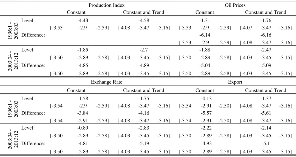
In table 4.1. we present our unit root test results. In table for each sub period – before and after war- and for each variables ADF test results were documented. Here we provide test statistics and critical values for %1, %5 and %10 confidence intervals. Before testing for stationarity we took natural logarithm of all variables in order to reduce the volatility of variables as suggested by literature. In addition during conducting ADF test we both test with constant and with constant and trend. Presence of these two separate tests increase the validity of obtained results. Before conduct ADF test we have to determine optimum lags that should be included to regression estimation of ADF test via VAR procedure. The included lags of variables for first period is as follows: industrial production index’s three

27

lag, for oil prices one lag, for exchange rate four lag, for export five lag included to the ADF test. In second period’s analysis; for industrial production index six lags, for oil prices, seven lags, for exchange rate five lags and for total export three lags were included to test procedure.

The test results of our analysis show that in first period except industrial production index all remaining variables have unit root. In other words, apart from industrial production index, all variables are not stationary in level. Henceforth, we took first difference of those variables and repeated the ADF test and we see that according to results we can reject null hypothesis of Augmented Dickey Fuller test, it means series became stationary after taking first difference of those variables. In short, except industrial production index all series are I(1) series, thus, they have unit root in level and it disappears after taking first difference. Therefore we going to proceed our analysis with first difference of all our variables for first period.

As next step we follow same procedure for second period’s variables. This time we cannot reject the null hypothesis of Augmented Dickey Fuller test results even for industrial production index. It means all series of second period have unit root, thus non stationary in level. Therefore we take first difference of all series and repeated the test and results indicate that all series became stationary after taking first difference. Their unit root has disappeared. In other words, all variables of second period are I(1). Henceforth we proceed our further analysis with first difference of second period’s variables.

All results obtained via ADF unit root test exhibited in table 4.1. For further queries about the results see below table.

28

Table 4.1.: Results of Augmented Dickey Fuller Test

Production Index Oil Prices

Constant Constant and Trend Constant Constant and Trend

1996:1 - 2003:03 Level: -4.43 -4.58 -1.31 -1.76 [-3.53 -2.9 -2.59] [-4.08 -3.47 -3.16] [-3.53 -2.9 -2.59] [-4.07 -3.47 -3.16] Difference: -6.14 -6.16 [-3.53 -2.9 -2.59] [-4.08 -3.47 -3.16] 2003:04 - 2013:12 Level: -1.85 -2.7 -1.88 -2.47 [-3.50 -2.89 -2.58] [-4.03 -3.45 -3.15] [-3.50 -2.89 -2.58] [-4.03 -3.45 -3.15] Difference: -4.85 -4.89 -5.04 -5.09 [-3.50 -2.89 -2.58] [-4.03 -3.45 -3.15] [-3.50 -2.89 -2.58] [-4.03 -3.45 -3.15]

Exchange Rate Export

Constant Constant and Trend Constant Constant and Trend

1996:1 - 2003:03 Level: -1.58 -1.75 -0.13 -1.37 [-3.54 -2.9 -2.59] [-4.08 -3.47 -3.16] [-3.54 -2.91 -2.50] [-4.08 -3.47 -3.16] Difference: -3.84 -4.16 -5.57 -5.61 [-3.54 -2.91 -2.59] [-4.08 -3.47 -3.16] [-3.54 -2.91 -2.50] [-4.08 -3.47 -3.16] 2003:04 - 2013:12 Level: -0.89 -2.83 -2.22 -2.14 [-3.50 -2.89 -2.58] [-4.03 -3.45 -3.15] [-3.50 -2.89 -2.58] [-4.03 -3.45 -3.15] Difference: -4.81 -5.19 -4.93 -5.1 [-3.50 -2.89 -2.58] [-4.03 -3.45 -3.15] [-3.50 -2.89 -2.58] [-4.03 -3.45 -3.15]

29

Our results of Unit Root test indicate that most of the variables of each sub period are I(1), in other words include unit root in level. During model specification we have to be sure about the existence of long relationship of those I(1) series. The reasons is if there is long run relationship between those non stationary variables we cannot follow VAR estimation procedure rather we prefer to use VECM analysis. The underlying reasons is VAR estimation assumes that there is no long run association between non stationary variables.

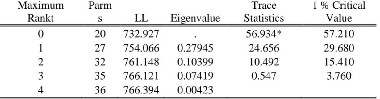
As mentioned above in methodology section we use Johensen cointegration analyses in order to determine whether I(1) series have long run relationship or not. In first period we put non stationary variables; log of export, log of oil prices and log of exchange rate to the Johensen cointegration analysis. For second period, according to results of unit root test, we put logarithm of industrial production index, logarithm of exchange rate, logarithm of crude oil prices and logarithm of export level to the cointegration analysis. For those variables optimum lag were determined via VAR estimation as done for Augmented Dickey Fuller Analysis.

Johensen cointegration test reveals those variables have how many number of cointegrated vectors if there is long run association. If the results indicate zero cointegrated vectors for variables it means the series are not cointegrated in other words, among series there are no long run relationship.

In our econometric analysis as data generator we use Stata throughout the examination and Stata’s cointegration feature is determining number of cointegration vectors of variables with consideration of both eigenvalues and trace statistics and marking the number of cointegrated vectors. According to results, in both periods the series have no cointegration vectors. In other words, examined series neither in before war period, nor after war period have long run relationship. The results of cointegration analysis of our series presented in table 4.2. and table 4.3. For further queries see below tables. Lack of cointegration vectors makes use proceed our analysis with VAR estimation.

30

Table 4.2.: Johensen Cointegration Test, Before War Maximum

Rank Parms LL Eigenvalue

Trace Statistics 1 % Critical Value 0 12 324.164 . 16.589* 35.650 1 17 329.311 0.11406 6.295 20.040 2 20 331.681 0.05423 1.556 6.650 3 21 332.459 0.01814 1

Table 4.3.: Johensen Cointegration Test, After War Maximum Rankt Parm s LL Eigenvalue Trace Statistics 1 % Critical Value 0 20 732.927 . 56.934* 57.210 1 27 754.066 0.27945 24.656 29.680 2 32 761.148 0.10399 10.492 15.410 3 35 766.121 0.07419 0.547 3.760 4 36 766.394 0.00423

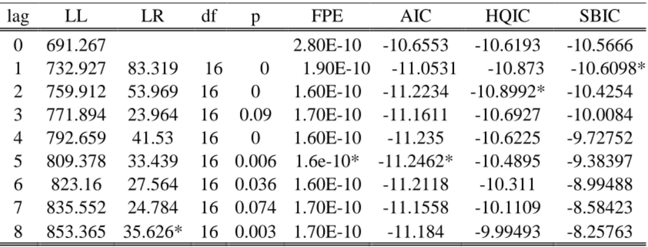
The next step of our econometric time series analysis is determination of optimum lags of variables that will be estimated via VAR estimation. As we describe above the Vector auto regression uses own lags of dependent variables as regressors in each equation. Therefore adding how many log to the regression equation should be determined before running regression. Adding less than optimum lag to the regression analysis will violate the validity of regression, contrary adding more lags than optimum will ruin degrees of freedom, thus significance of independent variables.

During determination of optimum lags as suggested by literature we follow Akaika Information Criteria (Akaike, 1974) and Hannah-Quinn Information Criteria (Hannah and Quinn, 1979) .

Same as cointegration analysis Stata marking the optimum lag according to each information criteria. And for first period Stata suggests adding only first lags of each variables to the VAR analysis according to Akaika Information Criteria and Hannah-Quinn Information Criteria. On the other hand, for second period (after war) used two information criteria’s suggest diverse lags. Hannah-Quinn

31

Information Criteria suggest adding two lags of variables to the analysis, yet Akaika Information Criteria suggests adding five lags of used variables to the VAR estimation. Here we decided to use AIK suggestion because the usage of AIK is much more wide compared to Hannah-Quinn Information Criteria.

The results of optimum lag selection procedures exhibited in table 4.4. and table 4.5. For further analyses see below tables.

Table 4.4.: Lag Order Selection: 1996:1 - 2003:3 Period

lag LL LR df p FPE AIC HQIC SBIC

0 373.494 9.00E-10 -9.4742 -9.42582 -9.35335 1 422.797 98.606 16 0 3.8e-10* -10.3281* -10.0862* -9.72385* 2 434.604 23.614 16 0.098 4.30E-10 -10.2206 -9.78519 -9.13291 3 446.376 23.544 16 0.1 4.80E-10 -10.1122 -9.48326 -8.54108 4 457.532 22.312 16 0.133 5.60E-10 -9.98801 -9.16553 -7.93345 5 465.528 15.991 16 0.454 7.00E-10 -9.78277 -8.76676 -7.24477 6 475.075 19.094 16 0.264 8.60E-10 -9.6173 -8.40777 -6.59588 7 487.119 24.088 16 0.088 1.00E-09 -9.51587 -8.11281 -6.01102 8 506.303 38.369* 16 0.001 1.00E-09 -9.59752 -8.00094 -5.60925

Table 4.5.:Lag Order Selection: 2003:4 - 2013:12 Period

lag LL LR df p FPE AIC HQIC SBIC

0 691.267 2.80E-10 -10.6553 -10.6193 -10.5666 1 732.927 83.319 16 0 1.90E-10 -11.0531 -10.873 -10.6098* 2 759.912 53.969 16 0 1.60E-10 -11.2234 -10.8992* -10.4254 3 771.894 23.964 16 0.09 1.70E-10 -11.1611 -10.6927 -10.0084 4 792.659 41.53 16 0 1.60E-10 -11.235 -10.6225 -9.72752 5 809.378 33.439 16 0.006 1.6e-10* -11.2462* -10.4895 -9.38397 6 823.16 27.564 16 0.036 1.60E-10 -11.2118 -10.311 -8.99488 7 835.552 24.784 16 0.074 1.70E-10 -11.1558 -10.1109 -8.58423 8 853.365 35.626* 16 0.003 1.70E-10 -11.184 -9.99493 -8.25763

After controlling for stationarity and presence of cointegration analysis we run VAR for our variables and for two periods separately. Here our aim is estimating the effect of oil prices on industrial production in before and after war period and compare the obtained coefficients. In this way we can say what happened to

32

association between industrial production index and crude oil prices after war; in addition to that we can compare the level of association between those variables. In our estimation, explained before we add further controls to our equation such as exchange rate and export level. Thanks to previous literature’s studies we know that those parameters are effecting industrial production index as well as crude oil prices.

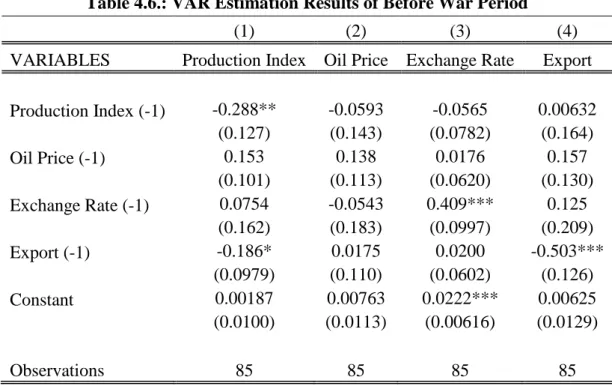
Before comparing the results of VAR estimation of sub periods we would like to interpret each estimation results separately. In this way we aim to provide detailed information about the association between variables in examined two periods. For before war period, during VAR analysis we put only first lags of our variables to the analyses. It was determined as a results of optimum lag determination procedure. Here we not only see the effects of oil prices, exchange rates and export on production index, but also we see those all variables effect on other variables. Because as we explained before in VAR procedure for each of variables separate regression analyses had been conducted.

According to results of first regression analysis (dependent variable is first difference of industrial production index), the first lag of industrial production index and export level have statistically significant effect on industrial production index. Remaining variables have no statistical significant impact on industrial production index. In addition to that we see from analysis, between industrial production index and export level there is negative association, with one percent change in export, industrial production index decreases twenty percent.

Despite lack of statistical significance as we examine the effect of crude oil prices on industrial production index we want to highlight the coefficient of oil prices. One percent increase in first lag of crude oil prices increase industrial production index fifteen percent. In other words, between first lag of oil prices and industrial production index there is positive association. See table 4.6. for details.

33

Table 4.6.: VAR Estimation Results of Before War Period

(1) (2) (3) (4)

VARIABLES Production Index Oil Price Exchange Rate Export Production Index (-1) -0.288** -0.0593 -0.0565 0.00632 (0.127) (0.143) (0.0782) (0.164) Oil Price (-1) 0.153 0.138 0.0176 0.157 (0.101) (0.113) (0.0620) (0.130) Exchange Rate (-1) 0.0754 -0.0543 0.409*** 0.125 (0.162) (0.183) (0.0997) (0.209) Export (-1) -0.186* 0.0175 0.0200 -0.503*** (0.0979) (0.110) (0.0602) (0.126) Constant 0.00187 0.00763 0.0222*** 0.00625 (0.0100) (0.0113) (0.00616) (0.0129) Observations 85 85 85 85

Standard errors in parentheses *** p<0.01, ** p<0.05, * p<0.1

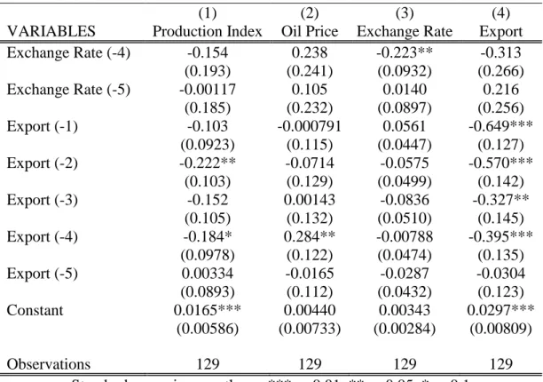
In table 4.7. we present the VAR estimation results of after war period. Same as regression estimation of before war period, here again we use same variables; log of industrial production index, log of crude oil prices, log of exchange rate and log of export volume. Here we use first difference of all variables due to unit root test results, as we touch upon above, in after war period all variables are non stationary in level but stationary in first difference. One another difference of this regression estimation is number of used lags in regression estimation. Our examination of optimum lag for regression estimation for post – war period, we see that five lags of all variables should be added to the model. Henceforth, instead of one lag as used in before war period regression here we put five lags of variables.

Our obtained results show that all added variables to the analysis have statistically significant impact on industrial production index but the significance level and the magnitude of the effect varies across variables.

34

Table 4.7.: VAR Estimation Results of After War Period

(1) (2) (3) (4)

VARIABLES Production Index Oil Price Exchange Rate Export Production Index (-1) -0.594*** 0.0940 -0.141** -0.387** (0.126) (0.157) (0.0609) (0.174) Production Index (-2) -0.247* 0.123 0.0631 -0.252 (0.128) (0.161) (0.0621) (0.177) Production Index (-3) -0.230* 0.172 0.0379 -0.173 (0.128) (0.160) (0.0618) (0.176) Production Index (-4) -0.279** -0.141 -0.0904 -0.0209 (0.129) (0.161) (0.0623) (0.178) Production Index (-5) -0.392*** 0.107 -0.0172 -0.485*** (0.128) (0.161) (0.0621) (0.177) Oil Price (-1) 0.0782 0.235** -0.00909 0.221** (0.0740) (0.0926) (0.0358) (0.102) Oil Price (-2) 0.255*** 0.187** -0.0130 0.259** (0.0733) (0.0917) (0.0355) (0.101) Oil Price (-3) 0.0108 -0.138 -0.0426 0.0435 (0.0748) (0.0935) (0.0362) (0.103) Oil Price (-4) 0.163** -0.120 0.0102 0.338*** (0.0746) (0.0932) (0.0361) (0.103) Oil Price (-5) -0.0152 0.00176 0.0470 0.0872 (0.0721) (0.0901) (0.0349) (0.0994) Exchange Rate (-1) -0.0165 -0.482** 0.494*** -0.240 (0.187) (0.234) (0.0907) (0.258) Exchange Rate (-2) -0.121 0.244 -0.395*** -0.140 (0.203) (0.253) (0.0981) (0.280) Exchange Rate (-3) -0.343* -0.235 0.152 -0.443 (0.204) (0.255) (0.0986) (0.281)

Standard errors in parentheses *** p<0.01, ** p<0.05, * p<0.1

First of all we see that lags of industrial production index has significant negative effect on current industrial production index. In details first and fifth lag has strongest effect on it when we consider significance level of coefficients. The effect of second, third and fourth lags are barely significant and the coefficient estimates are lower than first and fifth lag. On the other hand, when we focus on effect of crude oil prices on industrial production index we see that only second and fourth lags are effecting it significantly. Furthermore both significant or insignificant coefficient estimates are positive, thus we can say that between crude oil prices and industrial production index there is positive association in 2003-

35

2013 period. The effect of exchange rate on industrial production index is barely significant only at third lag and remaining coefficients are statistically insignificant. Despite lack of significance, coefficients indicate negative relationship between crude oil prices and industrial production index. When we look to export, similar to exchange rate only second and forth lags are statistically significant. Again sign of coefficients indicate reverse relationship between export and industrial production index, while export is increasing, industrial production index is declining.

Table 4.7. Continue

(1) (2) (3) (4)

VARIABLES Production Index Oil Price Exchange Rate Export

Exchange Rate (-4) -0.154 0.238 -0.223** -0.313 (0.193) (0.241) (0.0932) (0.266) Exchange Rate (-5) -0.00117 0.105 0.0140 0.216 (0.185) (0.232) (0.0897) (0.256) Export (-1) -0.103 -0.000791 0.0561 -0.649*** (0.0923) (0.115) (0.0447) (0.127) Export (-2) -0.222** -0.0714 -0.0575 -0.570*** (0.103) (0.129) (0.0499) (0.142) Export (-3) -0.152 0.00143 -0.0836 -0.327** (0.105) (0.132) (0.0510) (0.145) Export (-4) -0.184* 0.284** -0.00788 -0.395*** (0.0978) (0.122) (0.0474) (0.135) Export (-5) 0.00334 -0.0165 -0.0287 -0.0304 (0.0893) (0.112) (0.0432) (0.123) Constant 0.0165*** 0.00440 0.00343 0.0297*** (0.00586) (0.00733) (0.00284) (0.00809) Observations 129 129 129 129

Standard errors in parentheses *** p<0.01, ** p<0.05, * p<0.1

As last step of our VAR estimation analysis we would like to compare regression results of two sub periods. Here we aim to reveal difference between two period in terms of effects of crude oil prices on industrial production index. However we know that there are some shortages of this comparison and we are aware about these shortcomings.

36

First of all we know that coefficient estimates of VAR analysis do not indicate certain effects, in order to capture it decomposition and impulse response analysis is much more valid. However, difference between optimal lags between regression estimations and the different size of observations do not let us follow those methodologies. Henceforth we proceed our comparative analysis with comparison of coefficients with caution. Even in comparison of coefficients lack of several lag of variables in second period’s VAR estimation (second, third, forth and fifth lags) constraint our comparison. Nevertheless we can capture some of the differences of before and after war periods.

During comparison basically we compare coefficient estimates of two VAR estimations. Here we see that in first period first lag of production index do significantly effects itself, but in second period the effect is captured as negative. However the magnitudes of coefficients are slightly different. On the side of effect of crude oil prices on industrial production index we cannot capture any difference. In both regression analysis the coefficients of first lag of crude oil prices are statistically insignificant and positive. The only difference that we captured, the coefficient of crude oil prices in first period is higher than second period. Yet, the difference is not substantial enough. In addition to that in first period we cannot find statistically significant relationship between crude oil prices and industrial production index, however in second period’s VAR estimation in late lags we find statistically significant positive relationship between crude oil prices and industrial production index. In sum, our VAR estimation do not reveal any robust and significant change in relationship between industrial production index and crude oil prices. Overall the effect of oil prices on production index remains constant compared to before war period in after war period.

In our last part of results section we present our Grange causality test results. Granger causality test had been used to test the hypothesis of the absence of causal relationship between time series and according to Yıldırım and Öztürk (2014) it can be applied on the relationship between oil price and industrial production.

37

Same as before, we initiate our analysis with determination of optimum lags by using Akaika Information criteria. Then after, with optimum lags we run granger causality analysis for both directions, causality from crude oil prices to industrial production index and causality from industrial production index to crude oil prices. Our Granger causality test results were presented in table 4.8.

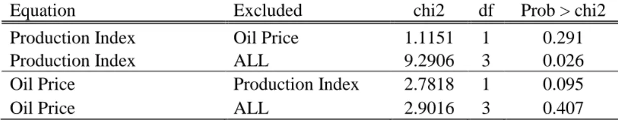
The null hypothesis of the test is lagged oil price does not cause industrial production index and the alternative hypothesis is oil prices does cause industrial production index. Here our chi-square value is 29 percent which is higher than 5 percent; thus we cannot reject null hypothesis rather accept null hypothesis. It means in before war period oil prices does not cause production index. In second Granger causality test we test for reverse causality, from production index to crude oil prices. Here the chi-square value is 9.5 percent it means in %5 critical value we accept null hypothesis but in %10 critical values we do reject null hypothesis. In other words, in %10 critical value, in before war period production index are Granger cause of oil prices. These results can be interpreted as in before war period between oil prices and industrial production index there is unilateral causal relationship; from production index to oil prices.

Table 4.8.: Granger Causality Test, Before War Period

Equation Excluded chi2 df Prob > chi2

Production Index Oil Price 1.1151 1 0.291

Production Index ALL 9.2906 3 0.026

Oil Price Production Index 2.7818 1 0.095

Oil Price ALL 2.9016 3 0.407

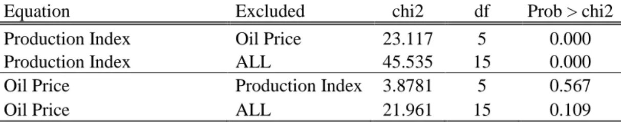
As second step of our analysis we run Granger causality test for same variables but for second period. Therefore we analyze the causal relationship between crude oil prices and industrial production index in after war period. The results were exhibited in table 4.9. and they indicate that for first test; we reject null. It means industrial production index does cause crude oil prices. On the other hand in second test we cannot reject null hypothesis. It means production index does not Granger cause of oil prices. These results say that there is unilateral relationship