published as:
Measurement of χ_{cj} decaying into pn[over ¯]π^{-} and
pn[over ¯]π^{-}π^{0}
M. Ablikim et al. (BESIII Collaboration)
Phys. Rev. D 86, 052011 — Published 26 September 2012
DOI:
10.1103/PhysRevD.86.052011
REVIEW COPY
NOT FOR DISTRIBUTION
Measurement of χ
cJdecaying into p¯
nπ
−and p¯
nπ
−π
0M. Ablikim1, M. N. Achasov5, O. Albayrak3, D. J. Ambrose39, F. F. An1, Q. An40, J. Z. Bai1, Y. Ban27, J. Becker2,
J. V. Bennett17, M. Bertani18A, J. M. Bian38, E. Boger20,a, O. Bondarenko21, I. Boyko20, R. A. Briere3, V. Bytev20,
X. Cai1, O. Cakir35A, A. Calcaterra18A, G. F. Cao1, S. A. Cetin35B, J. F. Chang1, G. Chelkov20,a, G. Chen1,
H. S. Chen1, J. C. Chen1, M. L. Chen1, S. J. Chen25, X. Chen27, Y. B. Chen1, H. P. Cheng14, Y. P. Chu1,
D. Cronin-Hennessy38, H. L. Dai1, J. P. Dai1, D. Dedovich20, Z. Y. Deng1, A. Denig19, I. Denysenko20,b,
M. Destefanis43A,43C, W. M. Ding29, Y. Ding23, L. Y. Dong1, M. Y. Dong1, S. X. Du46, J. Fang1, S. S. Fang1, L. Fava43B,43C, F. Feldbauer2, C. Q. Feng40, R. B. Ferroli18A, C. D. Fu1, J. L. Fu25, Y. Gao34, C. Geng40,
K. Goetzen7, W. X. Gong1, W. Gradl19, M. Greco43A,43C, M. H. Gu1, Y. T. Gu9, Y. H. Guan6, A. Q. Guo26,
L. B. Guo24, Y. P. Guo26, Y. L. Han1, F. A. Harris37, K. L. He1, M. He1, Z. Y. He26, T. Held2, Y. K. Heng1,
Z. L. Hou1, H. M. Hu1, T. Hu1, G. M. Huang15, G. S. Huang40, J. S. Huang12, X. T. Huang29, Y. P. Huang1,
T. Hussain42, C. S. Ji40, Q. Ji1, Q. P. Ji26,c, X. B. Ji1, X. L. Ji1, L. L. Jiang1, X. S. Jiang1, J. B. Jiao29, Z. Jiao14,
D. P. Jin1, S. Jin1, F. F. Jing34, N. Kalantar-Nayestanaki21, M. Kavatsyuk21, W. Kuehn36, W. Lai1, J. S. Lange36,
C. H. Li1, Cheng Li40, Cui Li40, D. M. Li46, F. Li1, G. Li1, H. B. Li1, J. C. Li1, K. Li10, Lei Li1, Q. J. Li1, S. L. Li1,
W. D. Li1, W. G. Li1, X. L. Li29, X. N. Li1, X. Q. Li26, X. R. Li28, Z. B. Li33, H. Liang40, Y. F. Liang31,
Y. T. Liang36, G. R. Liao34, X. T. Liao1, B. J. Liu1, C. L. Liu3, C. X. Liu1, C. Y. Liu1, F. H. Liu30, Fang Liu1,
Feng Liu15, H. Liu1, H. H. Liu13, H. M. Liu1, H. W. Liu1, J. P. Liu44, K. Y. Liu23, Kai Liu6, P. L. Liu29,
Q. Liu6, S. B. Liu40, X. Liu22, Y. B. Liu26, Z. A. Liu1, Zhiqiang Liu1, Zhiqing Liu1, H. Loehner21, G. R. Lu12,
H. J. Lu14, J. G. Lu1, Q. W. Lu30, X. R. Lu6, Y. P. Lu1, C. L. Luo24, M. X. Luo45, T. Luo37, X. L. Luo1,
M. Lv1, C. L. Ma6, F. C. Ma23, H. L. Ma1, Q. M. Ma1, S. Ma1, T. Ma1, X. Y. Ma1, Y. Ma11, F. E. Maas11,
M. Maggiora43A,43C, Q. A. Malik42, Y. J. Mao27, Z. P. Mao1, J. G. Messchendorp21, J. Min1, T. J. Min1,
R. E. Mitchell17, X. H. Mo1, C. Morales Morales11, C. Motzko2, N. Yu. Muchnoi5, H. Muramatsu39, Y. Nefedov20,
C. Nicholson6, I. B. Nikolaev5, Z. Ning1, S. L. Olsen28, Q. Ouyang1, S. Pacetti18B, J. W. Park28, M. Pelizaeus37,
H. P. Peng40, K. Peters7, J. L. Ping24, R. G. Ping1, R. Poling38, E. Prencipe19, M. Qi25, S. Qian1, C. F. Qiao6,
X. S. Qin1, Y. Qin27, Z. H. Qin1, J. F. Qiu1, K. H. Rashid42, G. Rong1, X. D. Ruan9, A. Sarantsev20,d,
B. D. Schaefer17, J. Schulze2, M. Shao40, C. P. Shen37,e, X. Y. Shen1, H. Y. Sheng1, M. R. Shepherd17, X. Y. Song1,
S. Spataro43A,43C, B. Spruck36, D. H. Sun1, G. X. Sun1, J. F. Sun12, S. S. Sun1, Y. J. Sun40, Y. Z. Sun1, Z. J. Sun1,
Z. T. Sun40, C. J. Tang31, X. Tang1, I. Tapan35C, E. H. Thorndike39, D. Toth38, M. Ullrich36, G. S. Varner37,
B. Wang9, B. Q. Wang27, D. Wang27, D. Y. Wang27, K. Wang1, L. L. Wang1, L. S. Wang1, M. Wang29,
P. Wang1, P. L. Wang1, Q. Wang1, Q. J. Wang1, S. G. Wang27, X. L. Wang40, Y. D. Wang40, Y. F. Wang1,
Y. Q. Wang29, Z. Wang1, Z. G. Wang1, Z. Y. Wang1, D. H. Wei8, J. B. Wei27, P. Weidenkaff19, Q. G. Wen40,
S. P. Wen1, M. Werner36, U. Wiedner2, L. H. Wu1, N. Wu1, S. X. Wu40, W. Wu26, Z. Wu1, L. G. Xia34,
Z. J. Xiao24, Y. G. Xie1, Q. L. Xiu1, G. F. Xu1, G. M. Xu27, H. Xu1, Q. J. Xu10, X. P. Xu32, Z. R. Xu40,
F. Xue15, Z. Xue1, L. Yan40, W. B. Yan40, Y. H. Yan16, H. X. Yang1, Y. Yang15, Y. X. Yang8, H. Ye1,
M. Ye1, M. H. Ye4, B. X. Yu1, C. X. Yu26, H. W. Yu27, J. S. Yu22, S. P. Yu29, C. Z. Yuan1, Y. Yuan1, A. A. Zafar42, A. Zallo18A, Y. Zeng16, B. X. Zhang1, B. Y. Zhang1, C. Zhang25, C. C. Zhang1, D. H. Zhang1,
H. H. Zhang33, H. Y. Zhang1, J. Q. Zhang1, J. W. Zhang1, J. Y. Zhang1, J. Z. Zhang1, S. H. Zhang1, X. J. Zhang1,
X. Y. Zhang29, Y. Zhang1, Y. H. Zhang1, Y. S. Zhang9, Z. P. Zhang40, Z. Y. Zhang44, G. Zhao1, H. S. Zhao1,
J. W. Zhao1, K. X. Zhao24, Lei Zhao40, Ling Zhao1, M. G. Zhao26, Q. Zhao1, Q. Z. Zhao9,f, S. J. Zhao46,
T. C. Zhao1, X. H. Zhao25, Y. B. Zhao1, Z. G. Zhao40, A. Zhemchugov20,a, B. Zheng41, J. P. Zheng1, Y. H. Zheng6,
B. Zhong1, J. Zhong2, Z. Zhong9,f, L. Zhou1, X. K. Zhou6, X. R. Zhou40, C. Zhu1, K. Zhu1, K. J. Zhu1,
S. H. Zhu1, X. L. Zhu34, Y. C. Zhu40, Y. M. Zhu26, Y. S. Zhu1, Z. A. Zhu1, J. Zhuang1, B. S. Zou1, J. H. Zou1
(BESIII Collaboration)
1 Institute of High Energy Physics, Beijing 100049, P. R. China
2 Bochum Ruhr-University, 44780 Bochum, Germany
3 Carnegie Mellon University, Pittsburgh, PA 15213, USA
4 China Center of Advanced Science and Technology, Beijing 100190, P. R. China
6 Graduate University of Chinese Academy of Sciences, Beijing 100049, P. R. China
7 GSI Helmholtzcentre for Heavy Ion Research GmbH, D-64291 Darmstadt, Germany
8 Guangxi Normal University, Guilin 541004, P. R. China
9 GuangXi University, Nanning 530004,P.R.China
10 Hangzhou Normal University, Hangzhou 310036, P. R. China
11 Helmholtz Institute Mainz, J.J. Becherweg 45,D 55099 Mainz,Germany
12 Henan Normal University, Xinxiang 453007, P. R. China
13 Henan University of Science and Technology, Luoyang 471003, P. R. China
14 Huangshan College, Huangshan 245000, P. R. China
15 Huazhong Normal University, Wuhan 430079, P. R. China
16 Hunan University, Changsha 410082, P. R. China
17 Indiana University, Bloomington, Indiana 47405, USA
18 (A)INFN Laboratori Nazionali di Frascati, Frascati, Italy;
(B)INFN and University of Perugia, I-06100, Perugia, Italy
19 Johannes Gutenberg University of Mainz, Johann-Joachim-Becher-Weg 45, 55099 Mainz, Germany
20 Joint Institute for Nuclear Research, 141980 Dubna, Russia
21 KVI/University of Groningen, 9747 AA Groningen, The Netherlands
22 Lanzhou University, Lanzhou 730000, P. R. China
23 Liaoning University, Shenyang 110036, P. R. China
24 Nanjing Normal University, Nanjing 210046, P. R. China
25 Nanjing University, Nanjing 210093, P. R. China
26 Nankai University, Tianjin 300071, P. R. China
27 Peking University, Beijing 100871, P. R. China 28 Seoul National University, Seoul, 151-747 Korea
29 Shandong University, Jinan 250100, P. R. China
30 Shanxi University, Taiyuan 030006, P. R. China
31 Sichuan University, Chengdu 610064, P. R. China
32 Soochow University, Suzhou 215006, China
33 Sun Yat-Sen University, Guangzhou 510275, P. R. China
34 Tsinghua University, Beijing 100084, P. R. China
35 (A)Ankara University, Ankara, Turkey; (B)Dogus University,
Istanbul, Turkey; (C)Uludag University, Bursa, Turkey
36 Universitaet Giessen, 35392 Giessen, Germany
37 University of Hawaii, Honolulu, Hawaii 96822, USA
38 University of Minnesota, Minneapolis, MN 55455, USA
39 University of Rochester, Rochester, New York 14627, USA
40 University of Science and Technology of China, Hefei 230026, P. R. China
41 University of South China, Hengyang 421001, P. R. China
42 University of the Punjab, Lahore-54590, Pakistan
43(A)University of Turin, Turin, Italy; (B)University of Eastern Piedmont, Alessandria, Italy; (C)INFN, Turin, Italy
44 Wuhan University, Wuhan 430072, P. R. China
45 Zhejiang University, Hangzhou 310027, P. R. China
46 Zhengzhou University, Zhengzhou 450001, P. R. China
a also at the Moscow Institute of Physics and Technology, Moscow, Russia b on leave from the Bogolyubov Institute for Theoretical Physics, Kiev, Ukraine
c Nankai University, Tianjin,300071,China
d also at the PNPI, Gatchina, Russia
e now at Nagoya University, Nagoya, Japan
f Guangxi University,Nanning,530004,China
Using a data sample of 1.06 × 10⁸
ψ′ events collected with the BESIII detector in 2009, the
branching fractions of χcJ → p¯nπ−and χcJ → p¯nπ−π0 (J=0,1,2) are measured1. The results for
measurements. The decays of χc1→ p¯nπ−and χcJ→ p¯nπ−π0are observed for the first time.
PACS numbers: 14.20.Gk, 13.75.Gx, 13.25.Gv
I. INTRODUCTION
Exclusive heavy quarkonium decays constitute an important laboratory for investigating perturbative Quantum Chromodynamics (pQCD). Compared to J/ψ and ψ′, relatively little is known concerning χcJ decays [1]. More
experimental data on exclusive decays of P-wave charmonia is important for a better understanding of the nature of χcJ states, as well as testing QCD based calculations. Although these states are not directly produced in e+e−
collisions, they are produced copiously in radiative decays of ψ′, with branching fractions around 9% [1]. The large ψ′
data sample taken with the Beijing Spectrometer (BESIII) located at the Beijing Electron-Positron Collider (BEPCII) provides an opportunity for a detailed study of χcJ decays.
Previous studies indicate that the Color Octet Mechanism (COM) [2], c¯cg → 2(q¯q) could have large effects on the observed decay patterns of these P-wave charmonia states [3–7]. To arrive at a comprehensive understanding about P-wave dynamics, both theoretical predictions employing the COM and new precise experimental measurements for χcJ many-body final states decays are required.
Also, the decays of χcJ with baryons in the final states provide an excellent place to investigate the production
and decay rates of excited nucleon N∗ states, which are a very important source of information for understanding the
internal structure of the nucleon [8].
The decays χcJ → p¯nπ− and χcJ→ p¯nπ−π0were studied by the BESII experiment with 14×106ψ′ events [9]. Due
to limited statistics and the detector performance, only χc0 → p¯nπ− and χc2 → p¯nπ− were observed and measured
with large uncertainties. A series of three-body and four-body decays of χcJ, including channels with similar final
states to ours such as p¯pπ0 and p¯pπ0π0, were measured by the CLEO-c Collaboration [10, 11].
In this paper, we present a measurement of χcJ decaying into p¯nπ−and p¯nπ−π0. The samples used in this analysis
consist of 156.4 pb−1 of ψ′ data corresponding to (1.06±0.04) × 108 [12] events taken at √s = 3.686 GeV/c2, and
42.6 pb−1 of continuum data taken at√s = 3.65 GeV/c2.
II. DETECTOR AND MONTE-CARLO SIMULATION
BESIII [13] is a major upgrade of the BESII experiment at the BEPCII accelerator [14] for studies of hadron spectroscopy as well as τ -charm physics [15]. The design peak luminosity of the double-ring e+e− collider, BEPCII,
is 1033 cm−2s−1 at center-of-mass energy of 3.78 GeV. The BESIII detector with a geometrical acceptance of 93%
of 4π, consists of the following main components: 1) a small cell, helium-based main draft chamber (MDC) with 43 layers. The average single wire resolution is 135 µm, and the momentum resolution for 1 GeV/c charged particles in a 1 T magnetic field is 0.5%; 2) an electromagnetic calorimeter (EMC) comprised of 6240 CsI (Tl) crystals arranged in a cylindrical shape (barrel) plus two end-caps. For 1.0 GeV/c photons, the energy resolution is 2.5% (5%) and the position resolution is 6 mm (9 mm) in the barrel (end-caps); 3) a Time-Of-Flight system (TOF) for particle identification (PID) composed of a barrel part constructed of two layers with 88 pieces of 5 cm thick, 2.4 m long plastic scintillators in each layer, and two caps with 48 fan-shaped, 5 cm thick, plastic scintillators in each end-cap. The time resolution is 80 ps (110 ps) in the barrel (end-caps), corresponding to a K/π separation by more than 2σ for momenta below about 1 GeV/c; 4) a muon chamber system (MUC) consisting of 1000 m2 of Resistive Plate
Chambers (RPC) arranged in 9 layers in the barrel and 8 layers in the end-caps and incorporated in the return iron yoke of the superconducting magnet. The position resolution is about 2 cm.
The optimization of the event selection and the estimation of backgrounds are performed through Monte Carlo (MC) simulation. The geant4-based simulation software boost [16] includes the geometric and material description
of the BESIII detectors and the detector response and digitization models, as well as the tracking of the detector running conditions and performance. The production of the ψ′ resonance is simulated by the MC event generator
kkmc[17], while the decays are generated by evtgen [18] for known decay modes with branching fractions being set to world average values [1], and by lundcharm [19] for the remaining unknown decays.
III. EVENT SELECTION
Charged-particle tracks in the polar angle range | cos θ| <0.93 are reconstructed from hits in the MDC. Only the tracks with the point of closest approach to the beamline within ±5 cm of the interaction point in the beam direction, and within 0.5 cm in the plane perpendicular to the beam are selected. The TOF and dE/dx information are used to form particle identification (PID) confidence levels for π, K and p hypotheses. Each track is assigned to the particle type that corresponds to the hypothesis with the highest confidence level. Exactly one proton and one π−, or one
antiproton and one π+ in the event are required in the analysis.
Photon candidates are reconstructed by clustering the EMC crystal energies. The minimum energy is 25 MeV for barrel showers (| cos θ| < 0.80) and 50 MeV for end-cap showers (0.86 < | cos θ| < 0.92). EMC cluster timing requirements are made to suppress electronic noise and energy deposits unrelated to the events.
A. Selection of ψ′→γχcJ, χcJ→pnπ¯ −
For the channel ψ′ → γχ
cJ, χcJ → p¯nπ−, at least one photon with energy greater than 80 MeV is required. To
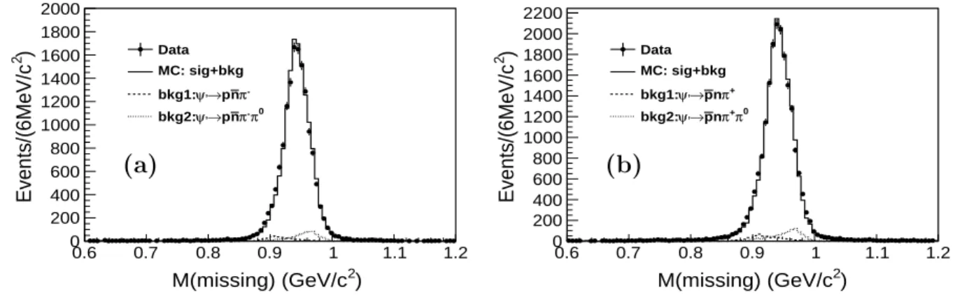
remove photons coming from interactions of charged particles or neutrons (antineutrons) in the detector, the angles between the photon and the antiproton, antineutron and other particles (pion, proton and neutron) are required to be greater than 30◦, 20◦, and 10◦, respectively. A one-constraint (1C) kinematic fit is performed under the ψ′ → γp¯nπ−
hypothesis, where the neutron (antineutron) is treated as a missing particle. For events with more than one isolated photon candidate, the combination with the smallest χ2
1C is retained, and χ21C< 10 is required. The distributions of
the recoiling mass against γpπ− and γ ¯pπ+ are shown in Fig. 1 (a) and Fig. 1 (b), respectively. Clear neutron and
antineutron peaks are observed around 0.938 GeV/c2.
) 2 M(missing) (GeV/c 0.6 0.7 0.8 0.9 1 1.1 1.2 ) 2 Events/(6MeV/c 0 200 400 600 800 1000 1200 1400 1600 1800 2000 Data MC: sig+bkg -π n p → , ψ bkg1: 0 π -π n p → , ψ bkg2:
(a)
) 2 M(missing) (GeV/c 0.6 0.7 0.8 0.9 1 1.1 1.2 ) 2 Events/(6MeV/c 0 200 400 600 800 1000 1200 1400 1600 1800 2000 2200 Data MC: sig+bkg + π n p → , ψ bkg1: 0 π + π n p → , ψ bkg2:(b)
FIG. 1: The distributions of mass recoiling (a) against γpπ−in ψ′
→ γp¯nπ−and (b) against γ ¯pπ+
in ψ′
→ γ ¯pnπ+
. Dots with error bars are data, and the solid histograms are the sum of signal and backgrounds, where the backgrounds are estimated from the inclusive MC and the continuum data at√s = 3.65 GeV/c2. The dominant
background contributions from ψ′
→ p¯nπ−(¯pnπ+
) and ψ′
→ p¯nπ−π0
(¯pnπ+
π0
) are shown as dashed and dotted lines, respectively.
An antineutron can form a cluster in the EMC with very high probability due to annihilation in the detector. To further purify the events with antineutrons and more than one photon, α < 15◦ is required, where α is the angle
between the expected antineutron direction and the nearest photon. Further, Mpπ−( ¯pπ+) > 1.15 GeV/c2 is required
to remove background events with Λ or ¯Λ. Finally, the transverse momentum for the proton or antiproton is required to be greater than 0.3 GeV/c due to the difference of the tracking efficiency at low transverse momentum between data and MC.
B. Selection of ψ′→γχ
cJ, χcJ→p¯nπ−π0
For ψ′→ γχ
cJ, χcJ → p¯nπ−π0, at least three isolated photons are required, where the photon isolation criteria are
the same as those in ψ′→ γχ
cJ, χcJ → p¯nπ−. π0candidates are selected from any pair of photon candidates that can
be kinematically fitted to the π0 mass and satisfy χ2< 20. There must be at least one π0candidate. A 1C kinematic
fit is performed to the ψ′→ γγγp¯nπ−hypothesis constraining the mass of the missing particle to that of the neutron,
where the three photons are a π0 candidate together with another photon. Kinematic fits are carried out over all
possible three-photon combinations. The kinematic fit with the smallest χ2
γγγp¯nπ− is retained, and χ2γγγp¯nπ− < 10 is
required. If there is more than one π0 candidate among the three photons, the pair with the invariant mass closest
to the π0 mass is assigned to be from the π0 decay. To further suppress backgrounds with final states γγp¯nπ− and
γγγγp¯nπ−, 1C kinematic fits are performed under γγp¯nπ−and γγγγp¯nπ−hypotheses,1and χ2γγγp¯nπ− < χ2γγp¯nπ− and
χ2
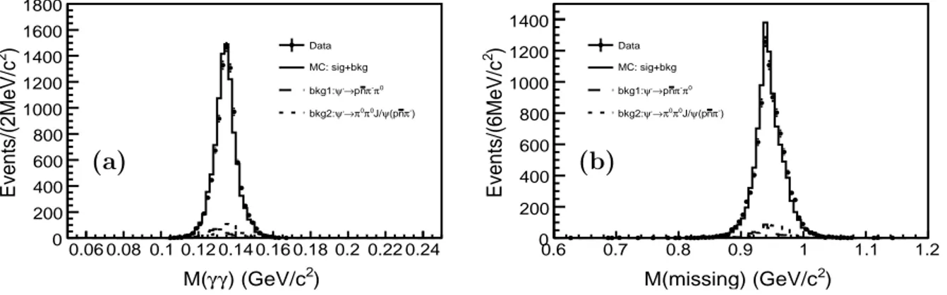
γγγp¯nπ− < χ2γγγγp¯nπ− are required. With the above selection criteria, the invariant mass of π0 and the distribution
of the recoiling mass against γpπ−π0in ψ′ → γp¯nπ−π0 are shown in Fig. 2 (a) and Fig. 2 (b), respectively. Similar
distributions are obtained in the charge conjugate channel.
) 2 ) (GeV/c γ γ M( 0.06 0.08 0.1 0.12 0.14 0.16 0.18 0.2 0.22 0.24 ) 2 Events/(2MeV/c 0 200 400 600 800 1000 1200 1400 1600 1800 Data MC: sig+bkg 0 π -π n p → , ψ bkg1: ) -π n (p ψ J/ 0 π 0 π → , ψ bkg2:
(a)
) 2 M(missing) (GeV/c 0.6 0.7 0.8 0.9 1 1.1 1.2 ) 2 Events/(6MeV/c 0 200 400 600 800 1000 1200 1400 Data MC: sig+bkg 0 π -π n p → , ψ bkg1: ) -π n (p ψ J/ 0 π 0 π → , ψ bkg2:(b)
FIG. 2: The invariant mass distribution of (a) γγ from π0 and (b) the distribution of recoiling mass against
γpπ−π0
in ψ′
→ γp¯nπ−π0
. Dots with error bars are data, and the solid histograms show the sum of signal and backgrounds, where the backgrounds are estimated from the inclusive MC and the continuum data at√s = 3.65 GeV/c2
. The dominant background contributions from ψ(2S) → p¯nπ−π0
and ψ(2S) → π0π0
J/ψ,J/ψ → p¯nπ−
are shown as dashed and dotted lines, respectively.
To suppress the background from ψ′ → π0π0J/ψ, for events with at least four photons, π0π0 combinations are
formed with any four photons, the one with the smallest ∆ =p(mγ1γ2− mπ0)2+ (mγ3γ4− mπ0)2 is selected, and
|Mrecoil− MJ/ψ| > 50 MeV/c2 is required, where Mrecoil is the mass recoiling against π0π0. To purify the channel
with antineutrons, the same requirement α < 15◦ as that for the channel ψ′ → γχ
cJ, χcJ → p¯nπ− is applied, and
the transverse momentum for proton or antiproton is required to be greater than 0.3 GeV/c in order to reduce the systematic uncertainty.
With the above criteria, clear χcJ signals are observed in the invariant mass distributions of p¯nπ−(¯pnπ+) in
χcJ → p¯nπ−(¯pnπ+) and of p¯nπ−π0(¯pnπ+π0) in χcJ → p¯nπ−π0(¯pnπ+π0), as shown in Figs. 3 (a) and (b) and Figs. 4
(a) and (b), respectively.
IV. BACKGROUND STUDIES
Background is investigated using both exclusive and inclusive MC samples, as well as continuum data. For ψ′ →
γχcJ, χcJ → p¯nπ−, a number of individual channels from the inclusive MC sample have been found to contribute to the
background. The following reactions have been found to be important: ψ′→ p¯nπ−π0(≈ 20% of the total background),
ψ′ → p¯nπ− (8%), ψ′ → π0π0J/ψ with J/ψ → p¯nπ− (1%), and ψ′ → γχ
cJ with χcJ → p¯nπ−π0 (4%). For the first
1 The two-photon combinations are pairs of photons from π0candidates, and the four-photon combination are pairs of photons from π0
) 2 ) (GeV/c -π n M(p 3.3 3.35 3.4 3.45 3.5 3.55 3.6 ) 2 Events/(5MeV/c 0 200 400 600 800 1000 1200 Exp.DataContinuum BG Resonant BG Sum of the BG
(a)
) 2 ) (GeV/c + π n p M( 3.3 3.35 3.4 3.45 3.5 3.55 3.6 ) 2 Events/(5MeV/c 0 200 400 600 800 1000 1200 1400 Exp.Data Continuum BG Resonant BG Sum of the BG(b)
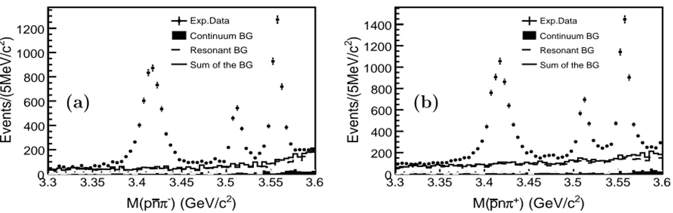
FIG. 3: Invariant mass distribution of (a) p¯nπ−for ψ′→ γp¯nπ−events, and of (b) ¯pnπ+
for the charge conjugate channel. Dots with error bars are data, and the filled histogram is the normalized non-resonant contribution estimated from continuum data at√s = 3.65 GeV/c2
. Resonant background, shown as the dashed histogram, is dominant and is estimated from MC. The sum of both background contributions is shown as the solid histogram.
) 2 ) (GeV/c 0 π -π n M(p 3.3 3.35 3.4 3.45 3.5 3.55 3.6 3.65 ) 2 Events/(5MeV/c 0 100 200 300 400 500 600 700 800 Exp.Data Continuum BG Resonant BG Sum of the BG
(a)
) 2 ) (GeV/c 0 π + π n p M( 3.3 3.35 3.4 3.45 3.5 3.55 3.6 3.65 ) 2 Events/(5MeV/c 0 100 200 300 400 500 600 700 800 900 Exp.Data Continuum BG Resonant BG Sum of the BG(b)
FIG. 4: Invariant mass distribution of (a) p¯nπ−π0 for the ψ′ → γp¯nπ−π0 channel, and of (b) ¯pnπ+π0 for the
charge conjugate channel. Dots with error bars are data, and the filled histogram is the normalized non-resonant
background contribution estimated from continuum data at√s = 3.65 GeV/c2
. Resonant background, shown as the dashed histogram, is dominant and is estimated from MC. The sum of both background contributions is shown as the solid histogram.
three background channels, the world average branching fractions listed in PDG [1] are used for normalization, and for χcJ → p¯nπ−π0, we use our own measurement as described in Sect. VI. The background originating from
non-resonant processes is estimated using a continuum data sample collected at a center-of-mass energy of 3.65 GeV/c2
after normalizing it to the integrated luminosity and the production cross section. The invariant mass distributions of p¯nπ−and of the charged conjugate state ¯pnπ+are shown in Figs. 3 (a) and (b), respectively. No peaking background
is observed in the signal region. Also ψ′ → γχ
cJ, χcJ → p¯nπ−π0 contains a number of individual background channels according to studies with
the inclusive MC sample. The dominant sources are the reactions ψ′ → p¯nπ−π0 (≈ 25% of the total background),
ψ′ → π0π0J/ψ with J/ψ → p¯nπ− (10%), and ψ′ → γχ
cJ with χcJ → p¯nπ− (1%). Again, for the latter channel
the branching fraction obtained from our own measurement is used for normalization (see Sect. VI); for the first two background channels the PDG [1] branching fractions are used. Additional background is studied using the inclusive MC sample, and the continuum data sample. The invariant mass distributions of p¯nπ−π0 and ¯pnπ+π0 are shown in
Fig. 4 (a) and Fig. 4 (b), respectively. Also in this case, no peaking background is observed in the signal region. It has been explicitly verified that the process ψ′ → γχ
cJ, χcJ → γJ/ψ with J/ψ → p¯nπ− or J/ψ → p¯nπ−π0 does not
V. INTERMEDIATE STATES
We have searched for potential intermediate N∗baryon resonances decaying into either pπ− or ¯nπ−. Such a study
is needed for correct modeling of χcJ → p¯nπ− and χcJ → p¯nπ−π0 in order to determine the efficiencies used in
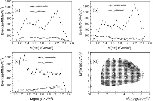
the calculation of the branching fractions of these decays, which is the main purpose of this work. Selecting χc0
events in the p¯nπ− decay mode, |M
p¯nπ−− Mχc0| < 45 MeV/c
2, the efficiency corrected pπ− and ¯nπ− invariant mass
distributions are shown in Fig. 5 (a) and Fig. 5 (b), respectively. Background contributions are also shown and are obtained from the sideband invariant mass region 45 MeV/c2 < |M
p¯nπ− − Mχc0| < 75 MeV/c
2. Fig. 5 (d) shows
in addition the corresponding Dalitz plot M2(¯nπ−) vs. M2(pπ−). The structures of the N∗ states at around 1.4
GeV/c2 and 1.7 GeV/c2 can be seen in both the pπ− and ¯nπ− invariant mass spectra as well as the bands in the
Dalitz plot. The p¯n invariant mass is shown in Fig. 5 (c). A large enhancement in the p¯n threshold region is observed, which is also visible as a diagonal band along the upper right-band edge in the Dalitz plot in Fig. 5 (d). A similar threshold enhancement has qualitatively been observed elsewhere, such as a p¯p threshold enhancement in B meson decays [20–25], ψ′ decays [26], and in the shape of the timelike electromagnetic form factor of the proton measured
at BaBar [27].
The peak at around 2.2 GeV/c2in both the pπ−and ¯nπ−invariant mass spectra is partly due to the reflection of the
threshold enhancement of p¯n. It might also be partly due to high mass N∗states, such as N∗(2190) or N∗(2220). The
same structures are observed in the charge conjugate mode of χc0 → ¯pnπ+ and the decays of χc1,2→ p¯nπ−. A partial
wave analysis is necessary to obtain more information about the N∗ components and the threshold enhancement in
the invariant mass distribution of p¯n.
) 2 ) (GeV/c -π M(p 1 1.2 1.4 1.6 1.8 2 2.2 2.4 2.6 ) 2 Events/(40MeV/c 0 200 400 600 800 1000 1200 1400 mass region c0 χ sideband c0 χ (a) ) 2 ) (GeV/c -π n M( 1 1.2 1.4 1.6 1.8 2 2.2 2.4 2.6 ) 2 Events/(40MeV/c 0 200 400 600 800 1000 1200 χc0 mass region sideband c0 χ (b) ) 2 ) (GeV/c n M(p 1.8 2 2.2 2.4 2.6 2.8 3 3.2 3.4 ) 2 Events/(40MeV/c 0 200 400 600 800 1000 χc0 mass region sideband c0 χ (c) 2 ) 2 )(GeV/c -π (p 2 M 0 1 2 3 4 5 6 7 2) 2 )(GeV/c -π n( 2 M 0 1 2 3 4 5 6 7 (d)
FIG. 5: The invariant mass distributions with the efficiency correction of (a) pπ−, (b) ¯nπ−, (c) p¯n and
(d) Dalitz plot for χc0 → p¯nπ− events. The dots with error bars are data, and the histograms are for
backgrounds obtained from sideband events.
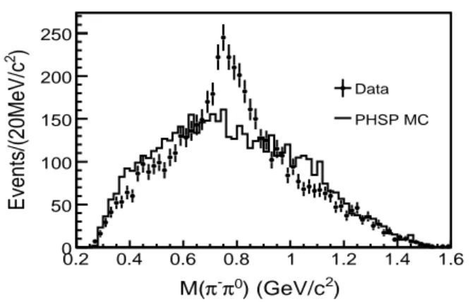
In χcJ → p¯nπ−π0, various two-body and three-body invariant mass distributions for events within the χcJ signal
region were investigated as well. No obvious N∗state is observed. The distributions are very similar to those of phase
) 2 ) (GeV/c 0 π -π M( 0.2 0.4 0.6 0.8 1 1.2 1.4 1.6 ) 2 Events/(20MeV/c 0 50 100 150 200 250 Data PHSP MC
FIG. 6: The invariant π−π0
mass distribution in χcJ → p¯nπ−π0 where a significant ρ signal is observed in the
data.
VI. SIGNAL EXTRACTION
Signal yields are extracted using unbinned maximum likelihood fits to the observed p¯nπ− and the p¯nπ−π0invariant
mass distributions. The following formula has been used for the fit:
2
X
i=0
BW (m; Mi; Γi) ⊗ G(m; σi) + BG, (1)
where BW (m; Mi; Γi) is the Breit-Wigner function for the natural lineshape of the χcJ resonance, BG represents
the background shape and is described by a third order Chebychev polynomial, and G(m; σi) is a modified Gaussian
function parameterizing the instrumental mass resolution, which was used by ZEUS Collaboration in ref [28] and expressed by: G(m; σi) = √1 2πσi e−(| m σi|) 1+(1+|1m σi| ) . (2)
In the fit, the natural widths of the χcJ states are fixed to the PDG [1] values, while their masses and corresponding
instrumental resolutions are floated. For ψ′ → γχ
cJ, χcJ → p¯nπ−, this fit is performed in the mass region of 3.30
GeV/c2≤ M(p¯nπ−) ≤ 3.60 GeV/c2, for the process ψ′ → γχ
cJ, χcJ → p¯nπ−π0 the mass region of 3.30 GeV/c2 ≤
3.64 GeV/c2 has been chosen.
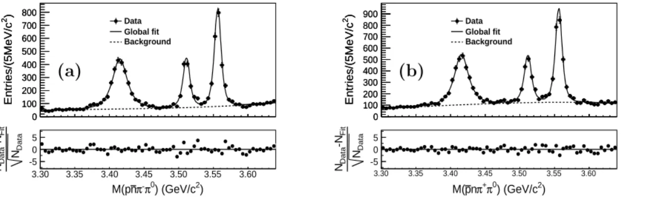
The fits to the p¯nπ− and ¯pnπ+ invariant mass distributions are shown in Fig. 7 (a) and 7 (b), respectively.
The corresponding fits to the p¯nπ−π0 and ¯pnπ+π0 invariant mass distributions are shown in Figs. 8 (a) and (b),
respectively.
MC samples for signal events have been generated to obtain the relevant detection efficiencies. In the underlying event generators, for the decay ψ′ → γχ
cJ an angular distribution proportional to 1+λ cos2(θ) has been assumed,
where θ is the angle between the direction of the radiative photon and the positron beam, and λ = 1, -1/3, 1/13 for J = 0, 1, 2, respectively, in accordance with expectations of electric dipole (E1) transitions. Since in the case of ψ′ → γχ
cJ, χcJ → p¯nπ−, structures have been observed in the pπ−, ¯nπ−, and p¯n invariant mass spectra (see
Sect. V), the decays of χcJ into p¯nπ− are generated taking these structures and the polar angle distribution of the
proton/neutron into account. The MC samples of χcJ → p¯nπ−π0 used to determine the detection efficiencies were
generated with a flat angular distribution, although a ρ± intermediate state is seen. To estimate the systematic
uncertainty associated with the missing ρ± intermediate state, a MC production of χ
cJ → p¯nρ− with the correct
angular distribution of ρ±→ π±π0has been generated (see Sect. VIII).
The χc0, χc1 and χc2 MC samples are finally weighted with the amplitudes observed in data, and the same fitting
process as that for data is performed to the mixed MC sample. The detection efficiencies of χcJ are calculated by
εcJ = NcJf it/N gen
cJ , where N f it
cJ is the number of χcJ events extracted from the fit, and NcJgenis the number of generated
) 2 Entries/(5MeV/c 0 200 400 600 800 1000 1200 1400 ) 2 Entries/(5MeV/c 0 200 400 600 800 1000 1200 1400 Data Global fit Background ) 2 ) (GeV/c -π n M(p 3.30 3.35 3.40 3.45 3.50 3.55 3.60 Data N Fit -N Data N -5 0 5
(a)
) 2 Entries/(5MeV/c 0 200 400 600 800 1000 1200 1400 1600 ) 2 Entries/(5MeV/c 0 200 400 600 800 1000 1200 1400 1600 Data Global fit Background ) 2 ) (GeV/c + π n p M( 3.30 3.35 3.40 3.45 3.50 3.55 3.60 Data N Fit -N Data N -5 0 5(b)
FIG. 7: Upper plot: The fit to the invariant mass distributions of (a) p¯nπ−and (b) the charge conjugate state
¯ pnπ+
. Dots with error bars are data, the solid curve is showing the fit to signal events, and the dashed line is the fitted background distribution. Lower plot: The distribution of NData√ −NF it
NData
from the fit.
) 2 Entries/(5MeV/c 0 100 200 300 400 500 600 700 800 ) 2 Entries/(5MeV/c 0 100 200 300 400 500 600 700 800 Data Global fit Background ) 2 ) (GeV/c 0 π -π n M(p 3.30 3.35 3.40 3.45 3.50 3.55 3.60 Data N Fit -N Data N -5 0 5
(a)
) 2 Entries/(5MeV/c 0 100 200 300 400 500 600 700 800 900 ) 2 Entries/(5MeV/c 0 100 200 300 400 500 600 700 800 900 Data Global fit Background ) 2 ) (GeV/c 0 π + π n p M( 3.30 3.35 3.40 3.45 3.50 3.55 3.60 Data N Fit -N Data N -5 0 5(b)
FIG. 8: Upper plot: The fit to the invariant mass distributions of (a) p¯nπ−π0 and (b) the charge conjugate state
¯ pnπ+
π0
. Dots with error bars are data, the solid curve is showing the fit to signal events, and the dashed line is the fitted background distribution. Lower plot: The distribution of NData−NF it
√
NData
from the fit.
VII. BRANCHING FRACTIONS
A. Branching fractions of χcJ→ p¯nπ−
The branching fractions of χcJ → p¯nπ− are calculated according to:
B(χcJ → p¯nπ−) = Nsig
Nψ′ × B(ψ′→ γχcJ) × εcJ, (3)
where Nsigis the number of signal events extracted from the fit to the invariant mass distribution, Nψ′ is the number
of ψ′ events, B(ψ′→ γχ
cJ) is the branching fraction of ψ′ → γχcJ as quoted in the PDG [1], and εcJ is the detection
efficiency. The results are summarized in the left column in Table I. The same calculation for the charge conjugate channel is performed, and the results are summarized in the right column.
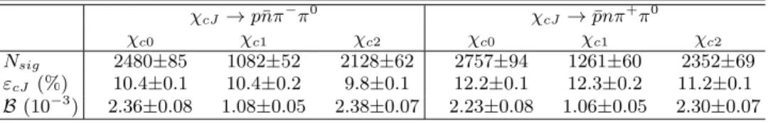
B. Branching fractions of χcJ → p¯nπ−π0
Considering the branching fraction of π0→ γγ, the branching fraction of χ
cJ → p¯nπ−π0 is calculated according to:
B(χcJ → p¯nπ−π0) =
Nsig
TABLE I: The number of signal events Nsig, the detection efficiency εcJ, and the branching fractions of χcJ → p¯nπ−, where
the errors are statistical only.
χcJ→ p¯nπ− χcJ→ ¯pnπ+
χc0 χc1 χc2 χc0 χc1 χc2
Nsig 5150±102 1412±58 3309±79 5808±121 1625±73 3732±89
εcJ (%) 38.6±0.2 35.9±0.3 39.2±0.2 40.9±0.2 40.7±0.3 41.2±0.2
B (10−3) 1.30±0.03 0.40±0.02 0.91±0.02 1.38±0.03 0.41±0.02 0.98±0.02
The results are summarized in the left column in Table II. The corresponding results for the charge conjugate channel are also shown in the right column.
TABLE II: The number of signal events Nsig, the detection efficiency εcJ and the branching fractions of χcJ→ p¯nπ−π0, where
the errors are statistical only.
χcJ→ p¯nπ−π0 χcJ → ¯pnπ+π0
χc0 χc1 χc2 χc0 χc1 χc2
Nsig 2480±85 1082±52 2128±62 2757±94 1261±60 2352±69
εcJ (%) 10.4±0.1 10.4±0.2 9.8±0.1 12.2±0.1 12.3±0.2 11.2±0.1
B (10−3) 2.36±0.08 1.08±0.05 2.38±0.07 2.23±0.08 1.06±0.05 2.30±0.07
VIII. ESTIMATION OF SYSTEMATIC UNCERTAINTIES
Several sources of systematic uncertainties are considered in the measurement of the branching fractions. These include differences between data and the MC simulation for the tracking algorithm, the particle identification (PID), photon detection, the kinematic fit, the requirement on the angle α, π0 reconstruction, the fitting procedure, and
the number of ψ′ events. Also possible imperfections in the description of intermediate resonances in the MC are considered.
a. Tracking and PID The uncertainties from tracking efficiency and PID are investigated using an almost
background-free control sample of J/ψ → p¯pπ+π− from (225.3 ± 2.8) × 108 J/ψ decays [29]. The tracking efficiency
is calculated with ǫ = Nf ull/Nall, where Nf ullis the number of events with all final tracks reconstructed successfully
and Nall is the number of events with three of them reconstructed while one track is missing. The PID efficiency is
the ratio of the number of selected events with and without PID. Both efficiencies are studied for pions and protons (antiprotons) as a function of transverse momentum and cos θ. The data - MC simulation difference for the tracking efficiency is estimated to be 1% per track. Therefore, a 2% uncertainty is taken for two-track events. For the PID efficiency, a 2% difference between data and MC is found for antiprotons, and 1% for any other charged particle. Therefore, 2% (3%) is taken as the systematic uncertainty for the final states including pπ− (¯pπ+).
b. Photon detection The uncertainty due to photon detection and photon conversion is 1% per photon. This
value is determined from a study using clean control samples, such as J/ψ → ρ0π0 and e+e− → γγ. Therefore, a
1% uncertainty is taken for the ψ′ → γχ
cJ → γp¯nπ− channel, while for the ψ′ → γχcJ → γp¯nπ−π0 channel, with 3
photons in the final state, a 3% uncertainty is taken.
c. Kinematic fit The systematic uncertainty stemming from the 1C kinematic fit is investigated using J/ψ → p¯nπ−
and J/ψ → p¯nπ−π0 events, where ¯n is treated as a missing particle with a mass of 0.938 GeV/c2. To obtain the
systematic uncertainty associated with the fit, pure control samples of J/ψ → p¯nπ− and J/ψ → p¯nπ−π0are selected,
and the 1C kinematic fit is applied to both charge states, both for data and MC. The efficiency of the 1C kinematic fit is estimated calculating the ratio of the number of events with and without the kinematic fit. From the two charge conjugate states, the larger difference between data and MC is taken as the systematic uncertainty. We assign an uncertainty of 2.9% for the kinematic fit in the case of p¯nπ−(π0) and 2.7% for ¯pnπ+(π0).
d. Angle α Another source of systematic uncertainty is the requirement on the angle αγ ¯n < 15◦. This uncertainty
is studied using the J/ψ → p¯nπ− sample and an uncertainty of 1.8% is assigned for this item.
e. π0reconstruction The uncertainty from the π0reconstruction is determined with a high purity and high statistics
the π+π− recoiling mass distribution with and without the standard π0 selection (1C kinematic fit). The data - MC
simulation difference has been measured to be 0.7%, and it has been verified that there is no dependence of this value from the π0 momentum and π0 polar angle.
f. Uncertainty from intermediate states As mentioned above, in χcJ → p¯nπ−, obvious N∗ intermediate states
and a p¯n threshold enhancement are observed in the invariant mass spectra of pπ− (¯nπ−) and p¯n (Fig. 5). To
account for these structures in the determination of the detection efficiency for χcJ → p¯nπ−, MC samples were
produced including these structures at the generator level. To determine the systematic error associated with this procedure, an alternative method is used, where the efficiency, including the effect of these structures for χcJ → p¯nπ−,
is determined by re-weighting MC events generated according to phase space by the ratio of data and MC events in the two-dimensional distribution of pπ− versus ¯nπ− invariant mass. The difference in the detection efficiencies
determined by the two methods is assigned as the systematic uncertainty. In χcJ → p¯nπ−π0, a strong ρ± signal is
observed in the π±π0invariant mass spectrum (Fig. 6), while MC samples used to estimate the detection efficiencies
are generated assuming phase space only. To study the effect of the intermediate state on the efficiencies, a sample of χcJ → p¯nρ− events is generated and analyzed. The efficiency difference between the two MC samples with and
without a ρ± intermediate state, (ε
pnππ0− εpnρ)/εpnππ0, is taken as the systematic uncertainty.
g. Fitting procedure As described above, the yields of the χcJ signal events are derived from fits to the invariant
mass spectra of p¯nπ− and p¯nπ−π0. To evaluate the systematic uncertainty associated with the fitting procedure, we
have studied the following aspects: (i) Fitting range: In the nominal fit, the mass spectra of p¯nπ− and p¯nπ−π0 are
fitted from 3.30 GeV/c2to 3.60 GeV/c2and from 3.30 GeV/c2 to 3.64 GeV/c2, respectively. We have changed these
intervals to 3.32−3.60 GeV/c2in the case of p¯nπ− and 3.32−3.62 GeV/c2 for p¯nπ−π0 events. The differences in the
finally obtained branching fractions by changing the fit intervals, are taken as the systematic uncertainties associated with the fit intervals. (ii) Signal lineshape: The partial width for an E1/M1 radiative transition is proportional to the cube of the radiative photon energy (E3
γ), which leads to a diverging tail in lower mass region. Two damping
functions have been proposed by the KEDR [30] and the CLEO [31] collaborations and have been used in addition to the standard approach in the formula describing the fit to the signal lineshape. Differences with respect to the fit not taking into account this damping factor have been observed, and the greater of the two differences is taken as the systematic uncertainty associated with the signal lineshape. (iii) Mass resolution parameterization: A single Gaussian formula instead of the modified Gaussian formula (Formula 2) has been used to describe the instrumental mass resolution. The resulting differences for the final branching fractions are taken as the systematic uncertainties. (iv) Mass resolution: Studies have shown that the χcJ mass resolutions, as simulated by MC, are underestimated.
To evaluate the systematic effects associated with this aspect, the invariant masses of p¯nπ− and p¯nπ−π0 in the MC
samples are smeared with a Gaussian function, where the width of this Gaussian depends on the invariant mass as well as on the channel. The same fitting processes as in the nominal cases are performed on the smeared mass spectra of p¯nπ− and p¯nπ−π0, and the detection efficiencies are recalculated. The efficiency difference between the smeared
and unsmeared case is taken as the systematic uncertainty. (v) Background shape: To estimate the uncertainties due to the background parameterizations, a second order instead of a third order Chebychev polynomial is applied in the fitting. Again, the difference between the two cases is used as an estimate of the systematic uncertainty.
h. Other systematic uncertainties The number of ψ′events is determined from an inclusive analysis of ψ′ hadronic
events and an uncertainty of 4% [12] is associated to it. The uncertainties due to the branching fractions of ψ′→ γχ cJ
and π0→ γγ are taken from the PDG [1]. A small uncertainty due to the statistical error of the efficiencies is also
considered.
In Table III a summary of all contributions to the systematic error is shown. In each case, the total systematic uncertainty is obtained by adding the individual contributions in quadrature.
IX. SUMMARY
Based on a data sample of 1.06×10⁸ ψ′ events collected with the BESIII detector, the branching fractions of
χcJ → p¯nπ− and χcJ → p¯nπ−π0 are measured for J = 0, 1, 2. The results are summarized in Table IV, where for
each branching fraction the first error is statistical and the second systematic. The product branching fractions of B(ψ′ → γχ
cJ) × B(χcJ → p¯nπ−) and B(ψ′ → γχcJ) × B(χcJ → p¯nπ−π0) are also summarized in Table V. For
χc0 → p¯nπ− and χc2 → p¯nπ−, the results are consistent with the world average values within one standard deviation,
while the precision is improved significantly. For the other χcJ decay modes, the branching fractions are measured
for the first time. A comparison of individual branching fraction shows good agreement between charge conjugate channels. The measurements improve the existing knowledge of the χcJ states and may provide further insight into
TABLE III: Summary of systematic errors (in %) for the branching fraction measurements of χcJ → p¯nπ−and χcJ → p¯nπ−π0. χcJ → p¯nπ− χcJ → ¯pnπ+ χcJ→ p¯nπ−π0 χcJ→ ¯pnπ+π0 χc0 χc1 χc2 χc0 χc1 χc2 χc0 χc1 χc2 χc0 χc1 χc2 MDC tracking 2.0 2.0 2.0 2.0 2.0 2.0 2.0 2.0 2.0 2.0 2.0 2.0 PID 2.0 2.0 2.0 3.0 3.0 3.0 2.0 2.0 2.0 3.0 3.0 3.0 Photon detection 1.0 1.0 1.0 1.0 1.0 1.0 3.0 3.0 3.0 3.0 3.0 3.0 Kinematic fit 2.9 2.9 2.9 2.7 2.7 2.7 2.9 2.9 2.9 2.7 2.7 2.7 αγ ¯n< 15◦ 1.8 1.8 1.8 - - - 1.8 1.8 1.8 - - -π0 reconstruction - - - 0.7 0.7 0.7 0.7 0.7 0.7 Intermediate states 5.3 6.2 8.2 4.0 1.2 5.0 3.0 1.7 0.7 1.5 1.8 2.3 Fit range 0.3 0.1 0.1 0.6 0.2 0.1 0.0 1.6 1.1 0.4 2.4 0.8 Signal lineshape 1.4 2.4 1.1 0.9 5.4 1.4 0.8 2.5 1.1 1.5 1.7 0.8 Resolution para. 1.9 4.6 3.0 3.1 5.3 3.1 2.1 5.5 1.7 0.4 4.9 2.2 Resolution diff. 0.3 1.4 1.3 0.5 0.2 0.7 1.9 1.9 1.0 0.8 2.4 1.8 Background shape 1.7 5.8 1.2 0.3 1.1 0.2 1.3 1.6 1.1 1.1 2.4 0.9 N(ψ′) 4.0 4.0 4.0 4.0 4.0 4.0 4.0 4.0 4.0 4.0 4.0 4.0 B(ψ′→ γχ cJ) 3.2 4.3 3.9 3.2 4.3 3.9 3.2 4.3 3.9 3.2 4.3 3.9 B(π0 → γγ) - - - 0.03 0.03 0.03 0.03 0.03 0.03 MC statistics 0.2 0.3 0.2 0.2 0.3 0.2 0.1 0.2 0.1 0.1 0.2 0.1 Total 9.1 12.5 11.5 8.6 10.8 9.5 8.6 10.6 8.3 7.9 10.6 8.8
their decay mechanisms. Based on the results of this work, detailed studies concerning the intermediate states may follow in the future.
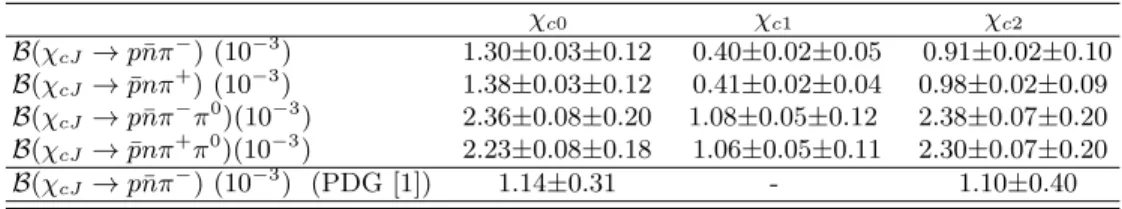
TABLE IV: Summary of branching fractions for χcJ → p¯nπ− and χcJ → p¯nπ−π0. The first errors are statistical, and the
second ones are systematic.
χc0 χc1 χc2 B(χcJ → p¯nπ−) (10−3) 1.30±0.03±0.12 0.40±0.02±0.05 0.91±0.02±0.10 B(χcJ → ¯pnπ+) (10−3) 1.38±0.03±0.12 0.41±0.02±0.04 0.98±0.02±0.09 B(χcJ → p¯nπ−π0)(10−3) 2.36±0.08±0.20 1.08±0.05±0.12 2.38±0.07±0.20 B(χcJ → ¯pnπ+π0)(10−3) 2.23±0.08±0.18 1.06±0.05±0.11 2.30±0.07±0.20 B(χcJ → p¯nπ−) (10−3) (PDG [1]) 1.14±0.31 - 1.10±0.40
TABLE V: Summary of the product branching fractions of ψ′→ γχ
cJ, χcJ → p¯nπ−and ψ′→ γχcJ, χcJ → p¯nπ−π0. The first
errors are statistical, and the second ones are systematic.
χc0 χc1 χc2 B(ψ′ → γχcJ) × B(χcJ→ p¯nπ−) (10−4) 1.26±0.02±0.11 0.37±0.02±0.04 0.80±0.02±0.09 B(ψ′→ γχ cJ) × B(χcJ→ ¯pnπ+) (10−4) 1.34±0.03±0.11 0.38±0.02±0.04 0.85±0.02±0.07 B(ψ′→ γχ cJ) × B(χcJ→ p¯nπ−π0)(10−4) 2.29±0.08±0.18 1.00±0.05±0.10 2.07±0.06±0.15 B(ψ′→ γχ cJ) × B(χcJ→ ¯pnπ+π0)(10−4) 2.16±0.07±0.16 0.98±0.05±0.10 2.01±0.06±0.16 X. ACKNOWLEDGMENTS
The BESIII collaboration thanks the staff of BEPCII and the computing center for their hard efforts. This work is supported in part by the Ministry of Science and Technology of China under Contract No. 2009CB825200; Na-tional Natural Science Foundation of China (NSFC) under Contracts Nos. 10625524, 10821063, 10825524, 10835001,
10875113, 10935007, 11125525, 10979038, 11005109, 11079030; Joint Funds of the National Natural Science Founda-tion of China under Contracts Nos. 11079008, 11179007; the Chinese Academy of Sciences (CAS) Large-Scale Scientific Facility Program; CAS under Contracts Nos. KJCX2-YW-N29, KJCX2-YW-N45; 100 Talents Program of CAS; Re-search Fund for the Doctoral Program of Higher Education of China under Contract No. 20093402120022; Istituto Nazionale di Fisica Nucleare, Italy; Ministry of Development of Turkey under Contract No. DPT2006K-120470; U. S. Department of Energy under Contracts Nos. DE-FG02-04ER41291, DE-FG02-91ER40682, DE-FG02-94ER40823; U.S. National Science Foundation, University of Groningen (RuG) and the Helmholtzzentrum fuer Schwerionen-forschung GmbH (GSI), Darmstadt; WCU Program of National Research Foundation of Korea under Contract No. R32-2008-000-10155-0.
[1] J. Beringer et al. (Particle Data Group), Phys. Rev. D 86, 010001 (2012). [2] H. D. Trottier, Phys. Lett. B 320, 145-151 (1994).
[3] H. W. Huang and K. T. Chao, Phys. Rev. D 54, 6850 (1996). [4] A. Petrelli, Phys. Lett B 380, 159 (1996).
[5] J. Bolz, P. Kroll and G. A. Schuler, Phys. Lett. B 392, 198 (1997). [6] S. M. H. Wong, Nucl. Phys. A 674, 185 (2000).
[7] S. M. H. Wong, Nucl. Phys. Eur. Phys. J. C 14, 643 (2000). [8] N. Isgur, arXiv:nucl-th/0007008v1, 6 Jul 2000.
[9] M. Ablikim et al. (BES Collaboration), Phys. Rev. D 74, 012004 (2006). [10] S. Athar et al. (CLEO Collaboration), Phys. Rev. D 75, 032002 (2007). [11] Q. He et al. (CLEO Collaboration), Phys. Rev. D 78, 092004 (2008). [12] M. Ablikim et al. (BESIII Collaboration), Phys. Rev. D 81, 052005 (2010).
[13] M. Ablikim et al. (BESIII Collaboration), Nucl. Instrum. Methods Phys. Res., Sect. A 614, 345 (2010).
[14] J. Z. Bai et al. (BESIII Collaboration), Nucl. Instrum. Methods Phys. Res., Sect. A 344, 319 (1994); 458, 627(2001). [15] D. M. Asner et al., Int. J. Mod. Phys. A 24, No. 1, 499 (2009).
[16] Z. Y. Deng et al., HEP & NP 30, 371 (2006).
[17] S. Jadach, B. F. L. Ward and Z. Was, Comp. Phys. Commu. 130, 260 (2000); S. Jadach, B. F. L. Ward and Z. Was, Phys. Rev. D 63, 113009 (2001). [18] R. G. Ping et al., HEP & NP 32, 599 (2008).
[19] J. C. Chen, G. S. Huang, X. R. Qi, D. H. Zhang, and Y. S. Zhu, Phys. Rev. D 62, 034003 (2000). [20] K. Abe et al. (Belle Collaboration), Phys. Rev. Lett. 88, 181803 (2002).
[21] B. Aubert et al. (BaBar Collaboration), Phys. Rev. D 72, 051101(R) (2005). [22] K. Abe et al. (Belle Collaboration), Phys. Rev. Lett. 89, 151802 (2002). [23] B. Aubert et al. (BaBar Collaboration), Phys. Rev. D 74, 051101(R) (2006). [24] J. T. Wei et al. (Belle Collaboration), Phys. Lett. B 659, 80 (2008).
[25] M. Z. Wang et al. (Bell Collaboration), Phys. Rev. Lett 92, 131801 (2004). [26] J. P. Alexander et al. (CLEO Collaboration), Phys. Rev. D 82, 092002 (2010). [27] B. Aubert et al. (BaBar Collaboration), Phys. Rev. D 73, 012005 (2006). [28] S. Chekanov et al. (ZEUS Collaboration), Eur. Phys. J. C 44, 351-366 (2005).
[29] M. Ablikim et al. (BESIII Collaboration), arXiv:1207.2865, accepted by Chinese Physics C. [30] V. V. Anashin et al. (KEDR Collaboration), arXiv:hep-ex/1012.1694v1, 8 Dec 2010. [31] R. E. Mitchell et al. (CLEO Collaboration), Phys. Rev. Lett. 102, 011801 (2009).