Selçuk J. Appl. Math. Selçuk Journal of Special Issue. pp. 149-161, 2011 Applied Mathematics
Interval Estimation for the Two-Parameter Pareto Distribution Based on Record Values
A. Asgharzadeh1, M. Abdi1, C. Ku¸s2
1Department of Statistics, Faculty of Basic Science, University of Mazandaran, Post
code 47416-1467, Babolsar e-mail: a.asgharzadeh@ um z.ac.ir
2Department of Statistics, Selcuk University, Konya, Turkey
e-mail: coskun@ selcuk.edu.tr
Abstract. This paper considers the interval estimation problem for the Pareto distribution based on record statistics. We present some exact confidence inter-vals and exact joint confidence regions for the parameters of Pareto distribution based on record statistics. One of the applications of the joint confidence re-gions of the parameters is to find confidence bounds for the functions of the parameters. In addition, the predictive interval of the future record based on the observed record values is also proposed. A Monte Carlo simulation is con-ducted to compare the proposed joint confidence regions. Finally, two numerical examples are given also to illustrate the methods proposed in this paper. Key words: Confidence interval; Joint confidence region; Pareto distribution; Prediction interval; Record statistics.
2000 Mathematics Subject Classification: 62G30; 62F25. 1. Introduction
Let X1, X2, ... be a sequence of independent and identically distributed (iid) random variables with cumulative distribution function (cdf) F (x) and proba-bility density function (pdf) f (x). An observation Xj is called an upper record value if Xj> Xi for every i < j. We assume that Xj occurs at time j, then the record time sequence is defined as
U (1) = 1, U (n) = min{j : j > U(n − 1), Xj> XU (n−1},
for n ≥ 2. The sequence {XU (n), n ≥ 1} provides a sequence of upper record statistics. An analogous definition can be given for lower record statistics. For more details see Arnold et al. (1998).
Record statistics can be viewed as order statistics from a sample whose size is determined by the values and the order of occurrence of the observations. It is of interest to note that there are situations in which only records are observed,
such as, in meteorology, hydrology, athletic events and mining. The statistical study of record statistics started with Chandler (1952) and has now spread in different directions. Detailed discussions of record statistics and its applications can be found in Arnold et al. (1998).
The Pareto distribution was originated by Pareto as a model for the distribution of income but is now used as a model in such widely diverse areas as insurance, business, economics, engineering, reliability and hydrology. A great deal of research has been done on estimation and properties of the Pareto distribution, and a very good summary of this work can be found in Johnson et al. (1994). The two-parameter Pareto distribution has the cumulative distribution function (1) F (x; ν, θ) = 1 −³ x
θ ´−ν
, x > θ > 0, ν > 0, and the probability density function
(2) f (x; ν, θ) = ν θ ³x θ ´−ν−1 , x > θ > 0, ν > 0.
This distribution is called Pareto type-I distribution (see, for example, Johnson et al. (1994)) with parameters θ and ν. Here the parameter ν is the shape parameter and θ is the scale parameter.
In the recent years, some work has been done on exact confidence intervals and regions for the parameters of Pareto distribution based on complete and censored samples. Chen (1996) proposed a joint confidence region for the para-meters of Pareto distribution based on complete and type-II censored samples. Wu (2003) obtained the confidence intervals for the parameters and percentile of Pareto distribution based on progressive type-II censoring with random re-movals. Kus and Kaya (2007) are derived an exact confidence region based on progressively type-II censored samples. Wu (2008) considered the interval estimation for the Pareto distribution based on a doubly type II censored sam-ple. Parsi et al. (2010) considered the simultaneous confidence intervals of the unknown parameters of Pareto distribution under progressive censoring. But up to now, no work has been done on confidence regions of the parameters of Pareto distribution based on records. In this paper, two methods are proposed to construct confidence intervals and joint confidence regions for the parameters of Pareto distribution based on upper records.
The paper is organized as follows: In Section 2, confidence intervals for ν and θ are considered based on upper records. We also present two exact joint confi-dence regions for the parameters ν and θ. Based on the joint conficonfi-dence region of these two parameters, a lower-confidence bound for the expected value E(X) and reliability function R(t) are also given in Section 2. In addition to the estimation of the two parameters, the predictive interval of the future record based on the observed upper records is derived in Section 3. In Section 4, a Monte Carlo simulation is conducted to compare the proposed joint confidence regions. Finally in Section 5, two numerical examples are given to illustrate the proposed confidence intervals and regions.
2. Confidence Intervals and Regions
Let XU (1) < XU (2) < · · · < XU (n) be the first n upper record values from the Pareto distribution with pdf (1). For notation simplicity, we will write Xi for XU (i). It can be shown that if let Yi = − ln[1 − F (Xi; ν, θ)] = ν ln(Xθi) (i = 1, 2, . . . , n), then Y1 < Y2 < · · · < Yn are the first n upper record values from a standard exponential distribution. Moreover, it is easy to show that
(3)
Z1= Y1, Z2= Y2− Y1,
n − 1
are iid random variables from a standard exponential distribution. This re-sult can be easily obtained from the joint pdf of Y1, Y2, . . . , Yn using a simple Jacobian argument (see Arnold et al. (1998)). Hence
(4) V = 2 Z1= 2 Y1,
has a chi-square distribution with 2 degrees of freedom and
(5) U = 2
n X i=2
Zi= 2 (Yn− Y1),
has a chi-square distribution with 2n − 2 degrees of freedom. We can also find that U and V are independent random variables.
Now, let us define
(6) T1=U/(2n − 2) V /2 = U (n − 1)V = 1 n − 1 µY n− Y1 Y1 ¶ , and (7) T2= U + V = 2Yn.
It is easy to show that T1 has an F distribution with 2n − 2 and 2 degrees of freedom and T2 has a chi-square distribution with 2n degrees of freedom. Furthermore, T1 and T2 are also independent (see Johnson et al. (1994), Page 350).
The distributions of the pivotal quantities U , V , T1and T2 are independent of parameters. These pivotal quantities are considered to obtain the confidence intervals and joint confidence regions for the parameters.
2.1. Confidence Intervals forν and θ
Making use of the pivotal quantity T1, we can construct the confidence interval for the scale parameter θ as follows:
Theorem 1. Suppose that X1 < X2 < · · · < Xn be the first n upper record values from the two-parameter Pareto distribution with parameters ν and θ. Then, a 100(1 − α)% confidence interval for θ is given by
⎛ ⎝X1 exp ⎡ ⎣− ln ³ Xn X1 ´ (n − 1)F1−α(2n − 2, 2) ⎤ ⎦ < θ < X1 ⎞ ⎠ ,
where F1−α(2n − 2, 2) is the upper 1 − α percentile of F distribution with 2n − 2 and 2 degrees of freedom.
Proof. From (6), we know that the pivot T1 = 1 n − 1 µ Yn− Y1 Y1 ¶ = 1 n − 1 ∙ln(X n) − ln(X1) ln(X1) − ln(θ) ¸ ,
has an F distribution with 2n − 2 and 2 degrees of freedom. Hence, we have P (F1−α(2n − 2, 2) < T1< ∞) = 1 − α, equivalently, P ⎛ ⎝X1 exp ⎡ ⎣− ln ³ Xn X1 ´ (n − 1)F1−α(2n − 2, 2) ⎤ ⎦ < θ < X1 ⎞ ⎠ = 1 − α.
This completes the proof. ¤ Let χ2
α(r) be the upper α critical value of the χ2distribution with r degrees of freedom. Based on the pivotal quantity U , we can obtain a confidence interval for the shape parameter ν as follows:
Theorem 2. Suppose that X1 < X2 < · · · < Xn be the first n upper record values from the two-parameter Pareto distribution with parameters ν and θ. Then a 100(1 − α)% confidence interval for the shape parameter ν is
à χ21−α 2(2n − 2) 2 ln(Xn X1) < ν < χ 2 α 2(2n − 2) 2 ln(Xn X1) ! .
Proof. From (5), we note that
U = 2 (Yn− Y1) = 2 ν ln µ Xn X1 ¶ ,
has a chi-square distribution with 2n − 2 degrees of freedom. Hence, we have 1 − α = P³χ21−α 2(2n − 2) < U < χ 2 α 2(2n − 2) ´ = P Ã χ2 1−α 2(2n − 2) 2 ln(Xn X1) < ν < χ 2 α 2(2n − 2) 2 ln(Xn X1) ! . This completes the proof. ¤
2.2. Joint Confidence Regions forν and θ
Let us now discuss the joint confidence regions for the parameters ν and θ. By using the pivotal quantities U and V , we can construct a joint confidence region for the parameters ν and θ in the following theorem.
Theorem 3 (Method 1). Suppose that X1< X2 < · · · < Xn be the first n upper record values from a Pareto distribution with parameters ν and θ. Then, based on the pivotal quantities U and V , a 100(1 − α)% joint confidence region for ν and θ is determined by the following inequalities:
⎧ ⎪ ⎪ ⎪ ⎨ ⎪ ⎪ ⎪ ⎩ X1 exp " − χ2 1−√1−α 2 (2) 2ν # < θ < X1 exp " − χ2 1+√1−α 2 (2) 2ν # , χ2 1+√1−α 2 (2n−2) 2 ln(XnX1) < ν < χ2 1−√1−α 2 (2n−2) 2 ln(XnX1) .
Proof. Since V and U are independent and V = 2ν ln(X1/θ) ∼ χ2(2) and U = 2ν ln(Xn/X1) ∼ χ2(2n − 2), we have P³χ21+√1−α 2 (2) < V < χ21−√1−α 2 (2)´=√1 − α, and P³χ21+√1−α 2 (2n − 2) < U < χ 2 1−√1−α 2 (2n − 2) ´ =√1 − α. From these relationships, we obtain
P µ χ21+√1−α 2 (2) < 2ν ln(X1 θ ) < χ 2 1−√1−α 2 (2), χ21+√1−α 2 (2n − 2) < 2ν ln( Xn X1 ) < χ21−√1−α 2 (2n − 2) ¶ = √1 − α.√1 − α = 1 − α. Equivalently, P ⎛ ⎝X1exp ⎡ ⎣−χ 2 1−√1−α 2 (2) 2ν ⎤ ⎦ < θ < X1exp ⎡ ⎣−χ 2 1+√1−α 2 (2) 2ν ⎤ ⎦, χ2 1+√1−α 2 (2n − 2) 2 ln(Xn X1) < ν < χ2 1−√1−α 2 (2n − 2) 2 ln(Xn X1) ⎞ ⎠ = 1 − α.
Thus the theorem follows.
Now, by using the pivotal quantities T1 and T2, we can obtain another joint confidence region for the parameters ν and θ.
Theorem 4 (Method 2). Based on the pivotal quantities T1and T2, a 100(1− α)% joint confidence region for the parameters of ν and θ is given by:
⎧ ⎪ ⎨ ⎪ ⎩ X1 exp h − ln(Xn)−ln(X1) (n−1)F√ 1−α(2n−2,2) i < θ < X1, χ2 1+√1−α 2 (2n) 2 ln(Xnθ ) < ν < χ2 1−√1−α 2 (2n) 2 ln(Xnθ ) .
Proof. From (7), we know that
T2= 2 Yn= 2ν ln µ Xn θ ¶ ,
has a chi-square distribution with 2n degrees of freedom, and it is independent of T1. Hence, we have P (F√ 1−α(2n − 2, 2) < T1< ∞) = √ 1 − α, and P (χ21+√1−α 2 (2n) < T2< χ21−√1−α 2 (2n)) =√1 − α. From these relationships, we obtain
P µ F√ 1−α(2n − 2, 2) < 1 n − 1 ∙ ln(Xn) − ln(X1) ln(X1) − ln(θ) ¸ < ∞ , χ2 1+√1−α 2 (2n) < 2ν ln(Xn θ ) < χ 2 1−√1−α 2 (2n) ¶ = 1 − α. Equivalently, P µ X1 exp ∙ − ln(Xn) − ln(X1) (n − 1)F√ 1−α(2n − 2, 2) ¸ < θ < X1, χ21+√1−α 2 (2n) 2 ln(Xn θ ) < ν < χ21−√1−α 2 (2n) 2 ln(Xn θ ) ⎞ ⎠ = 1 − α.
The theorem follows. ¤
The joint confidence regions given in Theorems 3 and 4 can be used to find confidence bounds for any function of the parameters ν and θ. For example, Corollary 2, will be used to obtain a lower confidence bound for the expected value
E(X) = θν
of a two-parameter Pareto distribution and Corollary 3, will be used to obtain a lower confidence bound for the reliability function
R(t) = 1 − F (t) = µ t θ ¶−ν , t > θ > 0.
Note that E(X) and R(t) are increasing in θ. Thus, the next corollaries are useful for that purpose.
Corollary 1. Based on the pivotal quantities U and V , the following inequali-ties determine a 100(1 − α)% joint confidence region for ν and θ:
⎧ ⎪ ⎪ ⎨ ⎪ ⎪ ⎩ θ > X1exp µ −χ 2 √ 1−α(2) 2ν ¶ , χ21+√ 1−α 2 (2n−2) 2 ln(XnX1) < ν < χ21−√ 1−α 2 (2n−2) 2 ln(XnX1) .
Corollary 2. Suppose that X1< X2< · · · < Xn be the first n upper record values from a two-parameter Pareto distribution. Then, for any 0 < α < 1,
inf ν>1 ( ν ν − 1X1exp à −χ 2 √ 1−α(2) 2ν !) ,
is a 100(1 − α)% lower confidence bound for the expected value E(X), where the infimum is taken over the region
χ2 1+√1−α 2 (2n − 2) 2 ln(Xn X1) < ν < χ2 1−√1−α 2 (2n − 2) 2 ln(Xn X1) .
Corollary 3. Suppose that X1< X2< · · · < Xn be the first n upper record values from a two-parameter Pareto distribution. Then, for any 0 < α < 1,
inf ν (µ t X1 ¶−ν . exp à −χ 2 √ 1−α(2) 2 !) ,
is a 100(1 − α)% lower confidence bound for the reliability function R(t), where the infimum is taken over the region
χ21+√1−α 2 (2n − 2) 2 ln(Xn X1) < ν < χ21−√1−α 2 (2n − 2) 2 ln(Xn X1) .
3. Prediction Interval for the Future RecordXn+1
The problem of prediction of future record values based on observed record data is a problem of considerable interest. For example, while studying the record rainfalls or snowfalls, having observed the record values until the present time, we will be naturally interested in predicting the amount of rainfall or snowfall that is to be expected when the present record is broken for the first time in future (See Arnold et al. (1998), Chapter 5). Prediction of future records has been studied by many authors in view of classical and Bayesian framework. In this section, we present a prediction interval for the future record Xn+1based on the observed record values X1, . . . , Xn. Prediction intervals can be constructed by using the distributions of appropriate pivotal quantities.
Let us consider the pivotal quantity S as
S = (n − 1)(ln Xn+1− ln Xn) ln Xn− ln X1
.
Since S follows an F distribution with 2 and 2n − 2 degrees of freedom, we can construct a prediction interval for Xn+1as follows:
Theorem 6. Suppose that X1 < X2 < · · · < Xn be the first n upper record values from the Pareto distribution in (1). Then, for any 0 < α < 1, a 100(1 − α)% prediction interval for the future record Xn+1is given by
⎛ ⎜ ⎝Xn µX n X1 ¶F 1−α2(2,2n−2) n−1 , Xn µX n X1 ¶F α 2(2,2n−2) n−1 ⎞ ⎟ ⎠ .
Proof Since S ∼ F (2, 2n − 2), then we have 1 − α = P¡F1−α 2(2, 2n − 2) < S < F α 2(2, 2n − 2) ¢ = P µ F1−α 2(2, 2n − 2) < (n − 1)(ln Xn+1− ln Xn) ln Xn− ln X1 < Fα 2(2, 2n − 2) ¶ = P ⎛ ⎜ ⎝Xn µ Xn X1 ¶F1−α 2(2,2n−2) n−1 < Xn+1< Xn µ Xn X1 ¶F α 2(2,2n−2) n−1 ⎞ ⎟ ⎠ .
The proof is thus completed. ¤ 4. Simulation
In this section, we have carried out a Monte Carlo simulation to compare the proposed joint confidence regions. In this simulation, we randomly generate upper record sample X1< X2 < · · · < Xn, from the Pareto distribution with
(ν, θ) = (2, 1), (2.5, 1). We replicate the process 5000 times and then computed 95% confidence intervals and regions and the corresponding mean confidence length and confidence area. For various choices of n, the simulated average confidence length and confidence area are presented in Table 1. From Table 1, we observe that when n increases, the average confidence lengths for ν and θ, and the average confidence area for (ν, θ) in both Methods 1 and 2 are decreased. We also observe that Method 2 has better performance than method 1, since it provides the smaller confidence area.
For purpose of validations, simulation study is also performed to investigate the coverage probabilities of the proposed confidence intervals and regions. The simulation results for the coverage probabilities are shown in Table 2. The simulation results shows that the coverage probabilities of the exact confidence intervals for ν and θ, and joint confidence regions for (ν, θ) in Methods 1 and 2 are close to the desired level of 0.95 for all sample sizes. Hence, our proposed methods for constructing exact confidence intervals and regions can be used reliably.
5. Illustrative Examples
In this section, two examples are given to illustrate the proposed confidence intervals and regions. We apply the proposed methods to one of practical data set and another simulated data set.
5.1. Example 1 (Real data set):
We use the following data which represent the 8 record values of the average July temperature (in degree centigrade) of Neuenburg, Switzerland, during the period 1864-1993 [from Madi and Raqab (2004) and Arnold et al. (1998), Page 278)]
19 20.1 21.4 21.7 22 22.1 22.6 23.4.
As pointed out by Madi and Raqab (2004), the Pareto model in (1.1) is adequate for these data. To find the 90% confidence intervals for ν and θ, and the 90% joint confidence region for ν and θ, we need the following percentiles:
F0.90(14, 2) = 0.3667, F0.9487(14, 2) = 0.2703, χ20.0257(2) = 7.3225, χ20.9743(2) = 0.0521, χ20.05(14) = 23.6847, χ20.95(14) = 6.5706, χ20.0257(14) = 26.0247, χ20.9743(14) = 5.6622, χ20.0257(16) = 28.7468, χ20.9743(16) = 6.9453.
By Theorems 1 and 2, the 90% confidence intervals for θ and ν are obtained as (17.5194, 19) and (15.7723, 56.8533) with confidence lengths 1.4806 and 41.0811, respectively.
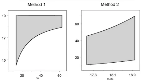
Figure 1. Joint confidence regions for ν and θ in Example 1.
By Theorem 3, the 90% joint confidence region for ν and θ is determined by the following inequalities: 13.5918 < ν < 62.6702, 19 exp ∙ −7.32252ν ¸ < θ < 19 exp ∙ −0.05212ν ¸ ,
with area 98.3986. By Theorem 4, the 90% joint confidence region for ν and θ is determined by the following inequalities:
6.9453
2 ln(23.4θ )< ν <
28.7468 2 ln(23.4θ ) 17.0196 < θ < 19,
with area 83.5585. Figure 1 shows the 90% joint confidence regions for ν and θ in both methods. By Theorem 6, the 90% predictive interval for the future record X9is obtained as (23.4359, 26.1538).
5.2. Example 2 (Simulated data):
In this example we consider a simulated sample of size n = 8 from the Pareto distribution with parameters θ = 3 and ν = 1.5. The simulated observations are as follows:
3.3303 4.0073 5.0572 12.0081 15.1123 22.8881 35.1399 93.8570. By Theorems 1 and 2, the 90% confidence intervals for ν and θ are obtained as (0.9072, 3.3303) and (0.9840, 3.5470) with confidence lengths 2.4231 and 2.5630, respectively.
By Theorem 3, the 90% joint confidence region for θ and ν is determined by the following inequalities: 0.8480 < ν < 3.8974, 3.3303 exp ∙ −7.32252ν ¸ < θ < 3.3303 exp ∙ −0.05212ν ¸ with area 7.1989.
Figure 2. Joint confidence regions for ν and θ in Example 2.
By Theorem 4, the 90% joint confidence region for ν and θ is determined by the following inequalities: 6.9453 2 ln(93.8570 θ ) < ν < 28.7468 2 ln(93.8570 θ ) 0.5705 < θ < 3.3303,
with area 7.6755. Figure 2 shows the 90% joint confidence regions for ν and θ in both methods. By Theorem 6, the 90% predictive interval for the future record X9 is obtained as (96.1901, 558.3962).
6. Aknowledgements:
The authors would like to thank the Department of Statistics at Selcuk Univer-sity and the Scientific and Technological Research Council of Turkey (TUBITAK) for supporting this research work.
References
1. Arnold, B.C., Balakrishnan, N., and Nagaraja, H.N, 1998. Records. New York, John Wiley and Sons.
2. Ku¸s, C. and Kaya, M.F, 2007. Estimation for the parameters of the Pareto distri-bution under progressive censoring. Commun. Statist.–Theor. Meth, 36: 1359-1365. 3. Chandler, K. N, 1952. The distribution and frequency of record values. J. Roy. Statist, Soc., B14: 220-228.
4. Chen, Z, 1996. Joint confidence region for the parameters of Pareto distribution. Metrika, 44: 191-197.
5. Johnson, N. L., Kotz, S., and Balakrishnan, N, 1994. Continuous Univariate Distribution, vol. 1. New York, John Wiley and Sons.
6. Madi, M.T. and Raqab, M.Z, 2004. Bayesian prediction of temperature records using the Pareto model. Environmetrics, 15: 701-710.
7. Parsi, S., Ganjali, M., and Sanjari Farsipour, N, 2010. Simultaneous Confidence Intervals for the Parameters of Pareto Distribution under Progressive Censoring. Com-mun. Statist.–Theor. Meth, 39(1): 94-106.
8. Wu, S-J, 2003. Estimation for the two-parameter Pareto distribution under pro-gressive censoring with uniform removals. J. Statist. Comput. Simul, 73: 125-134. 9. Wu, S.-F., 2008. Interval estimation for a Pareto distribution based on a doubly type II censored sample, Comput. Statist.& Data Analys, 52: 3779-3788.