Optimal row-column designs for treatment control comparisons

OPTIMAL HOW-COLUMN DESIGNS FOR

TREATMENT CONTROL COMPARISONS

A THESIS

SOBiVlITTED TO THE DEPARTMENT OF INDUSTRIAL

ENGINEERING

AND THE INSTITUTE OF ENGINEERING AND SCIENCE

OF BILKENT UNIVERSITY

IN PARTIAL FULFILLMENT C F THE REQUIREMENTS

FOR THE DEGREE OF

MASTER OF SCIENCE

By

Murat Aksu

Aucsust, 1997

OPTIMAL ROW-COLUMN DESIGNS FOR

TREATMENT CONTROL COMPARISONS

A THESIS

SUBMITTED TO THE DEPARTMENT OF INDUSTRIAL

ENGINEERING

AND THE INSTITUTE OF ENGINEERING AND SCIENCE

OF BILKENT UNIVERSITY

IN PARTIAL FULFILLMENT OF THE REQUIREMENTS

FOR THE DEGREE OF MASTER OF SCIENCE

Moro.+ ^Lsu.

Murat Aksu

August, 1997

TA

1

V Lf

■ A УІ

1

3 J ■/

I certify that I have read this thesis and that in my opinion it is fully adequate, in scope and in quality, as a thesis for the degree of Master of Science.

Assoc. (Advisor)

I certify that I have read this thesis and that in my opinion it is fully adequate, in scope and in quality, as a thesis for the degree of Master of Science.

Prof. T. Erkan Türe

I certify that I have read this thesis and that in my opinion it is fully adequate, in scope and in quality, as a thesis for the degree of Master of Science.

Assoc. Proi. Cemal Dinger

Approved for the Institute of Engineering and Sciences:

Prof. Mehmet Be

ABSTRACT

OPTIMAL ROW-COLUMN DESIGNS FOR TREATM ENT

CONTROL COMPARISONS

Murat Aksu

M.S. in Industrial Engineering

Supervisor: Assoc. Prof. Ülkü Gürler

August, 1997

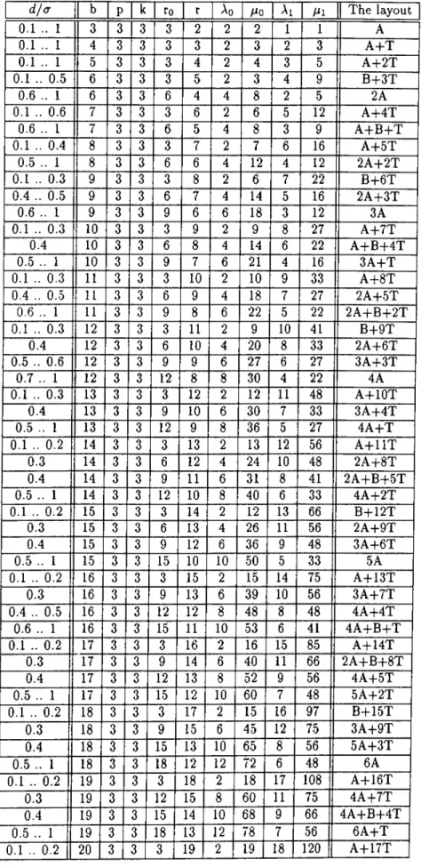
Problem of comparing a set of test treatments with a control or standard treatment arises in many applications. In the literature, there exist a number of alternative design settings available for the situation being considered. Problem is to choose one among several alternatives which is best in some sense. In this thesis, we considered two-way elimination of heterogeneity model with simultaneous confidence coefficient criterion. A procedure for making exact joint confidence statements for multiple comparisons with a control was described and some methods for the construction of the Balanced Treatment Row-Column Designs (B TR C D ’s) were given. Finally, tables of optimal BTR C D ’s were provided for practical range of parameter values.

Key words: Balanced Treatment Row-Column Designs, Optimal Designs, Simultaneous Confidence Interval Criterion, Two-Way Elimination of Hetero­ geneity.

ÖZET

TEST VE KONTROL ÖRNEKLERİNİN

KARŞILAŞTIRILMASI İÇİN OPTİMUM SATIR SÜTUN

DİZAYNLARI

Murat Aksu

Endüstri Mühendisliği Bölümü Yüksek Lisans

Tez Yöneticisi: Doç. Ülkü Gürler

Ağustos, 1997

Test örneklerini bir kontrol örneği ile karşılaştırma problemi ile bir çok uygulamada karşılaşılmaktadır. Göz önünde bulundurulan durum için kullanılabilecek pek çok alternatif dizayn vardır. Problem, alternatifler arasında en iyiyi, belirli bir ölçüte göre seçmektir. Bu çalışmada heterasyonun çift yönü eliminasyonu modeli ve eş anlı güven aralığı ölçütü kullanılmıştır. Eş anlı güven aralığının hesaplanması ve optimum dizaynların bulunması için araç ve metotlar tarif edilmiştir. Son olarak, heterasyonun iki yönlü eliminasyonu ve eş anlı güven aralığı kriterine göre optimum olan satır sütun dizaynlarının belirli parametre değerleri için tabloları verilmiştir.

Anahtar sözcükler·. Dengeli Dağılımlı Satır Sütun Dizaynları, Eş Anlı Güven Aralığı Ölçütü, Heterasyonun İki Yönlü Eliminasyonu, Optimum Dizaynlar.

To those who have filled my life with love

My sister Zeliha, and Esra

ACKNOWLEDGEMENT

I am indebted to Prof. T. Erkan Türe for his invaluable guidance, encouragement and above all, for the enthusiasm which he inspired on me during this study.

I would like to express my gratitude to Assoc. Prof. Ülkü Gürler due to her supervision, suggestions, and understanding to bring this thesis to an end.

I am indebted to Assoc. Prof. Cemal Dinçer for showing keen interest to the subject matter and accepting to read and review this thesis.

Finally, I would like to thank to my family and to my friends for their patience and help during the preparation of this thesis.

Contents

1 Introduction

1

2 Literature Review

9

3 Problem Definition and Preliminaries

13

3.1 Choice of D esigns... 14

3.1.1 Confidence Statement 16

3.2

Case of Negative Correlation... 17

3.2.1 Estimating Joint Probability When Correlation is Negative 17

3.3 Admissible and Optimal Designs... 19

4 Theoretical Results

24

4.1 Derivation of Variance and Correlation E xp ression s... 24

4.2 Results Concerning Variance and Correlation... 26

4.3 Construction of BTRC D ’s ... 29

5 Conclusion

34

A Tables of Optimal Designs

39

A .l Building Blocks For D e sig n s... 56

A.

1.1

Table K 2 P 2 ... 56 A.

1.2

Table K 2 P 3 ... 56 A. 1.3 Table K 2 P 4 ... .56 A. 1.4 Table K 2 P 5 ... 56 A. 1.5 Table K 3 P 3 ... 56 A.1.6 Table K 3 P 4 ... 57 A. 1.7 Table K 3 P 5 ... 57 A.

1.8

Table K 3 P 6 ... 57 A. 1.9 Table K 3 P 7 ... .59 A.1.10 Table K 4 P 4 ... 59 A.

1.11

Table K .5 P 5 ... 60

В Derivation of the Integral Expression

63

C Least Squares Normal Equations

66

List of Tables

A.l Table K2P2 . A.2 Table K2P2 . A.3 Table K

2

P

2

. A.4 Table K2P3 . A.5 Table K2P3 . A

.6

Table K2P4 . A.7 Table K2P5 . A

.8

Table K3P3 . A.9 Table K3P3 . A.IO Table K3P4 . A .ll Table K3P5 . A

.12

Table K3P6 . A.13 Table K3P7 . A.14 Table K4P4 . A.15 Table K4P4 . 45 45 46 47 48 49 50

IX

LIST OF TABLES

A.16 Table K 5 P 5 ... 54

Chapter 1

Introduction

Experimental design methods play an important role in process development and process trouble shouting as well as selection of best treatment among several alternatives or comparing new candidates to a control item.

Experiments are performed by investigators in virtually all fields of inquiry, usually to discover something about a particular process or system. Literally, an experiment is a test. A designed experiment is a test or series of tests in which purposeful changes are made to the input variables of a process or system so that we may observe and identify the reasons for changes in the output response.

As an example of an experiment, suppose that a metallurgical engineer is interested in studying the effect of two different hardening processes, oil quenching and salt water quenching, on an aluminum alloy. Here the objective of the experimenter is to determine the quenching solution that produces the maximum hardness for this particular alloy. The engineer decides to subject a number of alloy specimens after quenching. The average hardness of the specimens treated in each quenching solution will be used to determine which solution is the best.

to a large extend on the manner in which the data were collected. To illustrate this point, suppose that the metallurgical engineer in the above experimental setting used specimens from one heat in the oil quench and specimens from a second heat in the saltwater quench. Now, when the mean hardness is com­ pared, the experimenter is unable to say how much of the observed difference is the result of the quenching media and how much is the result of inherit differ­ ences between the heats. Indeed, the effects of quenching media and heat were confounded, that is both of these two factors affects the result simultaneously. Thus, the method of data collection has adversely affected the conclusions that can be drawn from the experiment.

According to Montgomery[16], while considering an experimental design like the one described above, number of important points should be answered:

• How many experimental units should be used and in what order should data be collected?

• What difference in average observed values among treatments will be considered important?

• What are the external sources of variability and how could it be dealt with?

• Are there other factors that might affect the results that should be in­ vestigated or controlled in the experiments?

CHAPTER 1. INTRODUCTION

2

Experimental design methods have found broad application in many disci­ plines. In fact, we may view experimentation as part of the scientific process. Generally, we learn through a series of activities in which we make conjectures about a process, perform experiments to generate data from the process, and then use the information from the experiment to establish new conjectures.

It is obviously the fact that if an experimental design is to be performed most efficiently, then a scientific approach to planning the experiment must be employed.

As a special type of design problem, there are certain experimental condi­ tions where one would like to compare the relative performance of some new treatments with respect to an existing standard or control treatment. Such a problem arises frequently in many biological, industrial and agricultural ex­ periments, for example, in screening experiments or in the beginning of a long term experimental investigation where it is initially desired to determine the relative performance of the new test treatments with respect to the control treatment. If it is possible to employ a completely randomized design this problem can be handled by using the available theory. However, most of the practical situations may require the blocking of experimental units so that the precision of the experiment can be improved and bias is reduced. Consider the following experimental situation; A certain type of alloy is used in the production of specific part of jet engines. The R&D department has developed four new types of alloy that can be used for the same purpose. Each of these four alloys could be easily produced in the existing production facility and can replace the present one if any one of them proved to be stronger. Suppose that we have four testing machines and five operators in order to conduct the exper­ iment. Since the variability between the machines and between the operators are suspected, the experiment must be designed to control such variability.

As a statistical problem, the question of how to compare the test treatments with the control cannot be answered unless it is asked in a more precise manner. To begin with it is needed to postulate a model for the response observed upon application of a treatment, test treatment or control, to an experimental unit. Three possible basic models could be considered: 0-way elimination of heterogeneity model in which all experimental units are homogeneous before application of treatments:

CHAPTER 1. INTRODUCTION

3

yij = fi + a i + €ij (

1

.

1

)

1

-way elimination of heterogeneity model in which experimental units can be divided into several homogeneous blocks:

CHAPTER 1. INTRODUCTION

2

-way elimination of heterogeneity model in which the experimental units con­ ceptually arranged according to rows and columns;

V ijh — fJ· + Cti + -| - T/i - f € i j h (1.3)

In models 1.1, 1.2 and 1.3 the y's denote observations obtained after applying treatment i to an experimental unit occurring in block j and row h, a{ rep­ resents the effect of treatment i, is the effect of column j , th. is the effect of row h and e’s are independent random error factors. In other words, a,, /

3

j, Th could be stated as the effect of new alloy i, machine j , and operator h respectively, in our alloy example.

For the one-way elimination of the heterogeneity model, the information matrix Cd of the differences oq — a,· is:

Cd = dtag(ro,ri,...,rp) - k~^NdN'^

Here, Nd = (r,j) is the incidence matrix of the design, r,· is the number of times treatment i occurs in the whole design and k is the common block size. Also, note that

ri = E r;,· J

=1

where r,jis the number of times treatment i is used in block j and the matrix. Let the matrix P

' ' 1 - 1 0 0

1 0 - 1 ... 0

P = (1.4)

1 0

0

...

- 1

be a p X (p 4-1) matrix. The matrix P C J^ P ' is called the covariance matrix

of the vector of the estimators of the contrast ao — cti, ...,Oio — ocp‘, here C^^ is a generalized inverse of

Cd-For the

2

-way elimination of the heterogeneity model the statistical setup consists of bk experimental units arranged in a ^ x

6

array, and the model of response under design is 1.3. Let

rij = number of times treatment i occurs in column j .

Sit = number of times treatment i occurs in row t.

n = E j= i rij,

Nd — {rij) , a (p + 1) X

6

matrix. Aid = (•Sit), a (p +

1

) X k matrix.

P is the p X (p + 1) matrix defined in 1.4

r<f = (^

0

,^

1

, ··, ^p)^ then information matrix Cj[7] is calculated as:

Cd = diag (ro,ri, ..,rp) - NdN'd - b~^MdM'd + {bk)~^ Vdr'd

CHAPTER 1. INTRODUCTION

Now we may be more precise about what we mean by comparing test treat­ ment with a control. In particular, because the primary goal is to determine which among the test treatments might be better than the control, we would like to estimate the magnitude of each oq — o, with as much precision as possi­

ble. More precise comparisons among test treatments found to perform better than the control at this initial stage is generally left to later experimentation. Under the assumptions made above, best linear unbiased estimators (BLUE’s)

«0

— o,· are used to estimate Oq — o,· under a given design d. In assigning

treatments to experimental units, the contrast ao — o, should be made to be estimable. A design satisfying this latter condition is said to be treatment con­ nected and obviously we should restrict our attention to such designs. Clearly there are a number of different designs available for the situation being con­ sidered here and we want to choose one of which is best in some sense. For example, one might choose a design that gives the minimal value among all available designs of ^ u a r ^ a o - a ,· ^ (1.5) or t = l A A max var I _{ao — a,} l<i<p ' ( 1.6 )

where var denotes the variance of Oq — â,·. A design which gives the minimum in 1.5 is called an A-optimal design and one which gives the minimum

CHAPTER 1. INTRODUCTION

in

1.6

is called an MV-optimal designs. These minimizations is usually not easy. As in other cases of the exact design theory, it is highly unlikely to obtain one method which is capable of producing A optimal design for arbitrary values of

b, k and p.

A-optimality and MV-optimality certainly appear to have very intuitive and appealing statistical interpretations and are the most widely used criteria for treatment-control comparisons type of design settings. Finding an A-optimal design corresponds to minimizing mean square error in inference and finding an MV-optimal design is analogous to finding a minimax procedure.

D-optimality selects a design which minimizes the determinant of the co- variance matrix. But for the problem of comparing test treatments with a control, the D-optimality criterion does not seem to be either an intuitively or statistically suitable criterion because the design it selects as being opti­ mal generally do not provide any more information about treatment-control comparisons than they do about comparisons among test treatments.

The structure of optimal designs for treatment-control comparisons seems to depend on the criterion used. Although A and MV-optimal designs are often the same, other criteria yield different designs, usually requiring either fewer or more replications of the control, but otherwise balanced with respect to test treatments. On the other hand, the A and MV-optimality criteria each have a natural and statistically meaningful interpretation as given above.

There are circumstances in which the experimenter is not sure whether to fit a one-way model or a two-way elimination of heterogeneity model to the data. For example, the performance of several technicians are being compared to the control and the days of the week as well as the hours within each day are the possible sources of heterogeneity. In such a situation it would be highly desirable to obtain a design which is A or MV-optimal under each of these models. Hedayat and Majumdar [10] has studied this aspect of the problem and gave some families of model robust designs.

CHAPTER 1. INTRODUCTION

experiments when the control is taken to be known and the interest lies in testing whether or not the overall effect of the new treatments are appreciable, we may want to contrast the average new treatment effect with the old one and minimize var(X],· a,/p — So) i =

1

, ..,p. This criterion seems appropriate to be called as J-optimality because it reduces to minimizing t r a c e — P'J , with J the p X p matrix of all ones. Certain J-optimal designs are also E- optimal, where E-optimality is defined as minimizing the maximum variance of all the estimated contrasts ]C»· Ci (ao — a,·) with =

1

. Thus although E-optimality does not appear to have a very natural statistical interpretation when there is a control, E-optimal plans may also deserve attention in some cases.

When we handle the design selection problem, we may choose among several optimality criteria. A- and MV-optimality criteria have statistically meaningful interpretation, i.e. both refer to minimizing suitable functions of the variances of the So — Si, they do not take their correlations into account. Thus the optimal designs derived would seem to be appropriate when the results of the experiment are to be reported in terms of the above point estimates accom­ panied by their estimated standard errors or in terms of separate confidence interval estimates of the Sq—S,·, i =

1

,.., p. However in many practical applica­ tions a simultaneous confidence region is much more appropriate than separate confidence intervals. In our alloy example, primary criterion is the parameter So — S, (test treatments with large values being preferred) but if there also is a secondary criterion such as cost then the precise rules for selection of the test treatments can not be stated in advance. For example, depending on the experimental results the two apparently “best” test treatments (in terms of the So — Si values) may be selected or even the third or fourth apparently “best” test treatment may be selected. A set of sim ultaneous confidence intervals guarantees a specified confidence coefficient regardless of which test treatments are selected and for which the corresponding confidence interval estimates are reported. Thus, from our viewpoint, the natural optimality criterion for the problem is that of maximizing the coverage probability of simultaneous confi­ dence region.

There are some reasons why simultaneous confidence interval criterion has been less popular in the literature than A-optimality and MV-optimality. First, because there is no closed form for the multivariate t or multivariate normal probability point, it is more difficult to establish that a design is "optimal”. Second, because the probability point is function of the yardstick d/cr, it is possible that for different values there will be different "optimal” designs.

In conjunction with the foregoing discussion, it was desirable to provide tables of best available (conjectured optimal) BTRC D ’s for the

2

-way elimina­ tion of the heterogeneity model and simultaneous confidence interval criterion. Most difficult part of the research was constructing BTR C D ’s. In order to solve the construction problem, we have used two main sources:

1

. Available BTRCD ’s in literature, and

2

. A method of construction described in the Chapter 4.

CHAPTER 1. INTRODUCTION

8

The organization of the thesis is as follows: In the next section a litera­ ture review will be given. The third chapter is devoted to the preliminaries and problem definition as well as definitions of admissibility and optimality. Derivation of the formulas for variance and correlation figures of treatment- control contrasts are provided in Chapter 4. Last chapter is reserved for con­ clusion and future directions of research. Tables of parameters of best available designs and building blocks for the construction of those designs will be pro­ vided in Appendix A. Finally, for the sake of completeness, derivation of a well known approximation for estimating the multi-variate normal probability integral and the normal equations for the least squares estimates will be given in the Appendix B.

Chapter 2

Literature Review

Comparing various makes or types of a certain item, called test treatments, with a currently used control treatment is a common problem. Examples of such items are different types of apparatus different brands of a drug, different types of fertilizer and different varieties of a plant. A study aimed toward a decision to retain or replace the current item will generally involve an exper­ iment and the use of some statistical methods. Results of these studies, the performance of the items will play an important role in reaching a decision. However, in some cases other factors may play a role as well.

Earliest works on this problem was carried out by Dunnet[

6

]. He also posed the problem of optimally allocating experimental units to control and test treat­ ments so as to maximize the probability associated with the joint confidence statement concerning the many-to-one comparisons between the mean of the control treatment and the means of the test treatments. But this paper and some other early works tacitly assumed that a completely randomized design was used. However, many practical situations may require the blocking of ex­ perimental units in order to cut down on bias and improve the precision of the experiment. In traditional design theory the comparisons of all treatment pairs are of equal importance. This leads to the use of such classical designs like balanced incomplete block designs (B IB ’s).

CHAPTER 2. LITERATURE REVIEW

10

However, BIB designs apparently are not appropriate for the present setting in which the control plays a distinguished role. Because of the special role played by the control treatment, Cox[5] proposed a design that employs the control treatment an equal number of times (once, twice,etc.) in each block, and the test treatments forming a BIB design in the remaining plots of the blocks; but no analytical details were given for this proposed design. A special case of Cox’s design (i.e. the control treatment is employed once in each block) is studied by Pesek[18]; he showed that this design is more efficient than a BIB design for comparisons with a control, but it is less efficient for pairwise comparisons between the test treatments. It is obviously the fact that even the Cox’s more general design is quite restrictive.

Bechhofer and Tamhane[3] were the first to study the problem of obtain­ ing optimal block designs for the treatment control comparison problem. But unlike the case of BIB designs, the structure of optimal designs for treatment- control comparisons seems to depend heavily on the criterion used. Bechhofer and Tamhane used the simultaneous confidence coefficient criteria. This cri­ teria chooses the design with maximum joint confidence coefficient. This ap­ proach not only requires the equal block sizes which are smaller than or equal to number of treatments and linear model described in

1.2

but also an ex­ tra assumption concerning the form of distribution of the random variables involved. The most commonly made distributional assumption is that of nor­ mality assumption. Bechhofer and Tamhane proposed a class of designs called balanced treatment incomplete block (B T IB ) designs. A B T IB is a design

d € C {b ,k ,p ), where C {b ,k ,p ) is the set of all designs for given

6

, k, p, if it satisfies the following conditions:

Aqi = Aq

2

= ... = Aop = Ao

Ai

2

— Ai3 — ... — A

21

— — Ap_i,p — Ai

In words, B T IB is a design d G C {b ,k ,p ) in which each treatment-treatment pair occurs equal number of times in the design and also each treatment-control pair occurs equal number of times. Bechhofer and Tamhane [1] used general linear statistical model for one-way elimination of heterogeneity and they also

CHAPTER 2. LITERATURE REVIEW

11

accepted the normality assumption. Optimal designs within BT IB D class for selected (p,k,b) where k < p is the number of plots per block, and b is the total number of blocks available for experimentation were provided. Their first work has a limited scope, optimal designs for p =

2

,..,

6

, A: =

2

and for p = .

3

, A: = 3 were provided. Bachhofer and Tamhane provided tables of ex- act(discrete), optimal designs for these (p,k) values for a range of b ’s. .A.lso tables of approximate (continuous) optimal designs are given for situations in which very large b-values are required. Following this work Bechhofer and Tamhane [

2

] improved their results for p = 4, A: = 3 and p = 5, A; = 3 . In their later study Bechhofer and Tamhane restricted the search for optimal designs using new definitions of admissibility, and providing strong and combinational admissibility concepts. In the first work for each of the six cases studied it is known that there are only two (non-equivalent) admissible generator designs while for the cases examined in the later study there are many (non-equivalent) admissible generator designs. The full set of generator designs is not known for either of these two cases, so the optimal designs given by Bechhofer and Tamhane are optimal relative to the generator designs which are known. How­ ever, they conjecture that they have enumerated all of the admissible generator designs for each of these later cases, and stated that if additional ones do exist the incremental gain that would be achieved by using full set in place of the set used in the study would be very small.

Since the main objective of the experiment is to compare the control treat­ ment with the test treatments, a criterion based on the variances of estimators of the comparisons between the control and each of the test treatments would be a meaningful measure. Majumdar and Notz [15] studied the A-optimality of B T IB designs. They also provided MV-optimal designs as well as A-optimal designs for the

1

-way elimination of the heterogeneity model. Main purpose of their article was to investigate further the method for finding A-optimal and A-efficient designs. Hedayat and Majumdar[

8

] gave an algorithm and a catalog of A- and MV-optimal designs. Hedayat and Majumdar[9] also provided fami­ lies of A- and MV-optimal designs. Optimal designs for the

2

-way elimination of the heterogeneity model was studied by Notz[17j. Majumdar[13] considered

CHAPTER 2. LITERATURE REVIEW

12

the problem of comparing test treatments with more than one controls.

Jacroux [

11

] [12] gave new methods for obtaining MV-optimal designs un­ der

1

-way elimination of the heterogeneity model. Hedayat and Majumdar [10] studied designs simultaneously optimal under both

1

- and

2

-way elimination of heterogeneity models. Cheng, Majumdar, Stufken and Tiire [4] gave new families of A- and MV-optimal designs and some approximations for one-way elimination models. Tiire[21] derived conditions under which BTR C D ’s are A-optimal. Later on Tiire[20] provided tables of A-optimal and A-efficient BTR C D ’s. Finally, Majumdar[14] explore connection between maximum joint confidence interval probability and A-optimality criteria for the

1

-way elimi­ nation of heterogeneity model.

Chapter 3

Problem Definition and

Preliminaries

In this chapter we will provide a rationale for choosing a design from a set of competing BTRC D ’s where p > 0. Also a procedure for calculating the joint confidence interval probability for the case of negative correlation will be offered. Throughout this study we considered one-sided confidence intervals where cr^ is assumed to be known. For the sake of simplicity, without losing generality, is considered as fixed and equal to one. Our purpose is to design an efficient experiment to compare p new treatments with the control. A design is a A: X

6

array of integers where k is the common block size and b is the total

number of blocks. Let the treatments be indexed by 0,1, ...,p with 0 denoting the control treatment and

1

,

2

, ...,p, where p >

2

and k < p, denoting the test treatments. Thus, N = kb is the total number of blocks available. We will consider the usual additive model:

Vijh — P T Tfi -f- £(j7i

with E Lo«^·’ = - YX=\'’’h -

0

; the Sijh are assumed to be i.i.d. A^(

0

,cr^) normal random variables with zero mean and variation. It is desired to make an exact joint confidence statement concerning the p differences ao — Qi based on their best linear unbiased estimators (BLU E’s) Qq — oci

(1

< z < p).

CHAPTER 3. PROBLEM DEFINITION AND PRELIMINARIES

14

3.1

Choice of Designs

Since the primary aim is to make a confidence statement that applies si­ multaneously to all of the p differences So — i =

1

p, our problem is regarded as being symmetric in these differences. A class of designs for which var (So — S,·) = r^cr^ (1 < * < p) and corr (So — S ,j, So — S,^) = pa^ , (*i ^ *

2

)

1

^ *

1

)

*2

^ p) will be considered where the parameters r and p depend on the design employed. For the one way elimination problem such designs are balanced treatment incomplete block(BTIB) designs. B T IB D ’s are balanced with respect to the test treatments. A design is a BTIBD if it satisfies the following conditions:

Ao =

-^01

=

^02

= Ai = Ai

2

= Ai3 = where Ao , Aj are some integers.

= Aop

— A

2

I — — Ap_l_p

In other words, each test treatment must appear with (i.e., in the same block as) the control treatment the same total number of times Ao over the design, and each test treatment must appear with every other test treatment the same number of times Aj over the design.

For the two way elimination model totally symmetric design class satis­ fying var

{64

— So) =

(1

< г < p) and corr (So — S ,j,S o — S,^) = pcr^ ,

(¿1

7

^ ¿

2,1

< ¿

1

,

¿2

< p) is the class of equireplicate balanced treatment row col­ umn designs (B TR C D ’s) where all treatments occur same number of times over the whole design. From now on all BTRCD’s considered will be equireplicate designs. Note that a design is called as a BTRCD if it satisfies the following conditions:

Ao — Aoi = Ao

2

= ... = Aop

Ai = Ai

2

= Ai3 = ... = A

21

= .. = Ap_i,p PO = POI = P02 = ··· = Pop

Pi = P12 = Pi3 = ··· = P21 = ·· = Pp-i.p

CHAPTER 3. PROBLEM DEFINITION AND PRELIMINARIES

15

In words, each test treatment must appear with (i.e., both in the same block and the same row as) the control treatment the same total number of times Aq

and Ho respectively over the design, and each test treatment must appear with (i.e., both in the same block and the same row as) every other test treatment the same number of times Ai and hi over the design.

Remark 1

Definitions o f B T IB D and BTR CD place no restriction on

r,,

the

number o f replications o f the test treatment used over the whole design. This implies that a design can be B T IB or BTR CD without the r,·

(1

< i < p) being

equal. As an example o f such a B T IB consider the following design fo r which

(p, k, b) = (4,3,8) and Ao ■=

2

—

₂

_{with r\ — r}

₂

₌₌

₇₃

_{= 4 and T}

₄

_{— 5;}

’

0 0 0 0 1 1 1 2

'

0 0 0

4

2 2

3 3

1 2

3 4 3 4 4 4 _

But fo r the BTRCD having an example :is not that easy even if we do restrict ourselves with equireplicate designs. Because a BTRCD should be both columnwise and rowwise symmetric. Additional constraints fo r the po and p\ force r i ’s to be equal in most o f the cases.

The specific multiple comparisons with the control (MCC) problem which is considered during our study is that of obtaining joint one-sided confidence intervals of the form

0^0 — Oil > C(o — cci — d (1 ^ ^ p)

for given values of (p, k, b) when is known, and d is a specified yardstick asso­ ciated with the width of the confidence interval. The probability P associated with this joint confidence statement can be written as

P = Pr {ao - a, > So - 5,· - d ; {1 < * < p }}

= Pr{Z,· < d/rcT ;

{ l < i < p } }

d/r(T -f

- L

n

n

.=1

$

\/l - p (f) (z) dz

(3.1)

CHAPTER 3. PROBLEM DEFINITION AND PRELIMINARIES

16

where {Z\, ...■,Zp) has a p —v ariate equicorrelated standard normal distribution with common correlation p and common variation and ^ (-) denotes the standard univariate normal distribution function. For given p and specified d/r the probability of 3.1 depends on the BTRCD considered only through p and

T. This fact gives us an opportunity to compare BTR C D ’s among themselves.

3.1.1 Confidence Statement

Joint 100(1 — a) percent confidence intervals for the «o — «i

(1

< z < p) are given below.

One-sided Confidence Intervals: When is unknown, the joint one-sided confidence intervals are defined by Bechhofer and Tamhane[3] as the following:

OtQ- a , >ao - “ i (I < i < p ) (3.2)

In 3.2, denotes the upper equicoordinate a point of the p-variate equicor­ related central t distribution with common correlation p, and with degree of freedom v.

When is known , the joint one-sided confidence intervals are obtained by replacing t[°^pTSx, in 3.2 by z^'^lra where (= t[°lp for v = oo) denotes the upper equicoordinate a point of the p-variate equicorrelated standard normal distribution with common correlation p.

Derivation of the probability statement in 3.1 is provided in Appendix B with a related proof which states that correlation matrix of a BTRCD is positive definite if p € ( —

1

/ (n —

1

) ,

1

).

CHAPTER 3. PROBLEM DEFINITION AND PRELIMINARIES

17

3.2

Case of Negative Correlation

During our search for the optimal designs we have faced with a few negatively correlated designs. Although there are a negligible number of such BTR C D ’s, we have to find a method to estimate joint confidence interval probability for those negatively correlated designs. Both in the one-way elimination of hetero­ geneity and two-way elimination of heterogeneity models the joint probability

P could be calculated relatively easily from

P = P {Zj < d/Ta,{\ < i < p)}

= y 5»''|(x>/p-h d/Tcrj/^/n^ d $ (x )

where {Z i, Z

2

, Zp) has a p-variate equicorrelated standard normal distribu­ tion with common correlation p and $ (·) denotes the standard normal cu­ mulative distribution function. Unfortunately, this easy to calculate formula valid for evaluating joint probability integral only for the cases in which p >

0

. For the one-way elimination problem all possible designs have positive corre­ lation coefficient, so above formula is valid and sufficient. However, during the search for BTRCD ’s a few design came-up with negative correlation coef­ ficient especially when k = p and b is close to p value, and hence the above solution for calculating the joint probability coefficient could not be used for these cases. For these rare cases Monte Carlo method may be used to approx­ imate the numerical value of the multinormal integral. To describe a method that applies to the multivariate normal distribution, a sufficient procedure to generate n-dimensional normal variates X i, X

2

·, Xn with an N (p, J2) distri­ bution should be available. Following well known method is proper to generate

n-dimensional normal variates with an N (p ,J2 ) distribution

3.2.1 Estimating Joint Probability When Correlation is

Negative

The method described below is a well known procedure in literature for gen­ erating X i, X

2

,...,Xn from an A’ (p ,E ) distribution with arbitrary but fixed

CHAPTER 3. PROBLEM DEFINITION AND PRELIMINARIES

18

H and ( which is positive definite). This method depends on the following result; for every n x n positive definite matrix there exist an n x n matrix T = (tij) such that TT' = In general, matrix T is not unique. How­ ever if we restrict our attention to the subclass of all lower triangular matrices, then it is unique and could be obtained easily.

P rop osition

1

// Z! = ( (j,j) is an n X n positive definite matrix^ then there exists a unique lower triangular matrix T = (tij) satisfying TT' = Further­ more the elements o f T are given by:

t {j — til = til =

0

for all

1

< ¿ < j < n, for i =

2

, n >/cqi7 <7,1

v / ^

J - l 1/2 for ;■ =

2

,...,n k=l 1/2 - Y2 Lrtjr for j < n and i - 2 , . . . , n k=l

If Z is Nn (0, In) and T is the matrix obtained by applying the above propo­ sition then X = T Z + has an Nn {fJ·, Z ) distribution. Consequently to gener­ ate independent random variates X\, X

2

·, ■■■, Xn according to this distribution, the following algorithm[19] may be used.

1

. Compute T = (i,j)

2. Input i?;v, n, n = (/Í

1

, and T = (i,■_,·), where R^ is the number of replications, n denotes the dimension of the multivariate normal dis­ tribution and T is the unique lower triangular matrix obtained by using above proposition.

CHAPTER 3. PROBLEM DEFINITION AND PRELIMINARIES

19

3. Generate (Z i, Z

2

, Zt) (which are (pseudo) independent A'’ (

0

,

1

) vari­ ates) and apply the transformation = T Z +

i.e. compute

n

Xit — ^ “1“ for

2

— 1, 72 j=l

and then form Xt = {X u, ■■,Xnt)' 4. Repeat step 3 for i =

1

, ..,Ri,/.

Above procedure will facilitate the generation of multivariate normal data. After having an efficient method to generate n-variate random variable one can follow the following steps to estimate the probability P.

1. Input 72, /

2

, X;, and Rn.

2

. Set Ct = 0.

3. Repeat the following procedure for f =

1

to N\ Generate n-variate normal and observe

\ Ct if Xt A,

Ci+l = <

[ Ci -I-1 \{ X t e A

4. Compute /= Cn/Riv where / is the estimator of the probability.

3.3 Admissible and Optimal Designs

In search for the optimal design for given {p,k,b), it is desirable to eliminate from consideration certain designs that are uniformly dominated by other de­ signs and hence cannot be optimal for any d/cr. Following section contains the definition of such inadmissible design as well as optimal and admissible designs

CHAPTER 3. PROBLEM DEFINITION AND PRELIMINARIES

20

D efinition

1

For given (p,k) and specified d /a the B T R C D that achieves the

highest join t confidence coefficient P with the specified b is said to be optimal fo r that value o f b.

D efinition

2

I f fo r given (p, k) we have two designs D\ and D^with param eters

(i>i,T^,pi) and (b

2

, T f , p

2

) with bi <

62

» (ind if fo r every d and a , D\ yields a

confidence coefficient P at least as large as (larger than) that yielded by D

2

when bi <

62

(61

=

62

), then D

2

is inadmissible with respect to D\.

D efinition 3 I f a design is not inadmissible, then it is admissible. I f fo r given

(p, kj we have two designs D\ and D

2

with parameters (bi,Tf, pi) and (

62

, t|, P

2

)

and if bi =

62

, = r|, and p\ = p

2

, then D\ and D

2

are called as equivalent designs.

D efinition 4 For given (p, k) consider two B T R C designs D\ and D

2

with param eters {bi,r^,pi) and {b

2

, r f , p

2

), respectively. Design D

2

is inadmissible with respect to design D\ if and only if bi <

62

» ^ Pi — P'i

least one inequality is being strict.

From 3.1 it could be easily seen that as a decreases for fixed d and p, the confidence coefficient P increases. Monotonicity with respect to p follows from a special case of Sleepian’s inequality which states that if X = ( X i , X „ ) has an Nn { Pi Jl ) distribution with positive definite defined in B .l then

S “tl

CHAPTER 3. PROBLEM DEFINITION AND PRELIMINARIES

21

E x am p le

1

For an application o f these definitions consider the following two

designs fo r (

6

, p ,k ) = {

10

,

6

,

6

): Di = Do — ^

0 0 0 1 6

5 4 3

2 1

2 0 0 0 1 6

5 4 3

2

0 6 0 0 2 1

3 5 4 3

0 0 1 0

4 3

2 6

5 4 ')

6

4 3

2 0 0 0 1 6

5 3 5 4 5

0 0 0 2

1 6

_>

0 0 0 0 1 6 2

5 3 4

0 0 0 0

3 4

6 1 2

5

1 0 0 0 0

5 3

2

4

6

6 0 0 1

4

0 0

3 5

2

*»

0

5 4

2 0 0 0 6 1

3

0

3

2

5

0 0 0

4

6 1

j

0

, fiO =

21

^ 5, =

8

and ro = 24, r =

6

, A,

0

=:

10

, po = 24, Ai

and r| = 0.24708, p

2

= 0.285714 fo r D^. Since b\ =

62

, < r f, and pi > p

2

then we can claim that design D

2

is inadmissible with respect to design D\.

D\ always yields larger joint confidence coefficient than D

2

, so we do not have to consider design D

2

in our search for optimal designs .

Having the optimality and admissibility criteria on hand, we have used the following procedure to determine the optimal designs for specific [p, k, b) and

d ja values. Note that the term optimal design refers to the best design among available alternatives. Since the full set of BTR C D ’s for given (p, k^ b) is not known, the optimal designs that we give are optimal relative to the BTRC D ’s known to us; however, we conjecture that we have enumerated all possible BTRC D ’s and if additional ones do exist the incremental gain that would be achieved by using the full set in place of our set would be very small.

CHAPTER 3. PROBLEM DEFINITION AND PRELIMINARIES

22

2. Find all BTRC D ’s for this combination of {p ,k ,b ) values. 3. Calculate and p for every design available.

4. Eliminate inadmissible designs from the set of candidate designs for op­ timality.

5. For d /a (typically) ranging from 0.1 to 1.0 calculate

P = Pr {ao — a i > olq — OLi — d {1 < * < p }} for each admissible BTRCD.

6

. The BTRCD with the highest value of P is optimal for that value of (p, A:, b) and d ja .

This procedure requires complete list of BTRCD’s for given (p, k, b). This is a much more difficult job than it was for the one-way elimination of the heterogeneity model. In the one-way model if D\ and D

2

are two B T IB D ’s with parameters (p, A:,

61

) , Aoi, An and (p ,k ,b

2

) , A

02

, A

12

respectively, then

Di U D

2

is also a BTIBD with parameters (p, A:,

61

-|-

62

) , Aq = Aqi -|- A

02

and

Ai = All + A

12

. Unfortunately, this is no longer the case for the BTRCD ’s. Union of two BTRC D ’s does not necessarily yield a new BTRCD. In order to explain this situation consider the following two BTRC D ’s. Note that all BTR C D ’s are also B T IB by definition.

Di =

D\ and D

2

are both BTRCD with parameters (p = 4, A: = 4

,61

=

6

) , Aqi =

6

, All = 1, Poi = 9, pii - 2 and (p = 4, A: = 4

,61

= 4), Aoi = 3, An = 2, poi - 3, pii = 2 respectively. Let Dz = D

\ 0

D

2

0 0 0 1 2 3 0 1 2 3 0 0 0 2 3 4 1 0 3 4 1 3 4 0 0 0 4 2 0 1 4 1 2 0 0 0 2 3 4 0 ■

0 0 0 1 2

3 ' ’

0 1 2

3 ‘

0 0 0 2

3 4 , D

2

=

1 0

3 4

1

3 4

0 0 0

4

2 0 1

_ 4

1 2 0 0 0

_

2

3 4

0

Dz =

CHAPTER 3. PROBLEM DEFINITION AND PRELIMINARIES

23

D

3

is a B T IB with (p = 4, = 4

,61

= 10), Aqi = 9, An = 3 , but it is clearly not a BTRCD . Hence the construction of all possible designs remains as a difficult task. Once this is done, a computer program could be used to evaluate the joint confidence interval coefficients and so, optimal design for each (p, k, b)

Chapter 4

Theoretical Results

4.1

Derivation of Variance and Correlation E x ­

pressions

In this section variance and correlation expressions for estimators of treatment control contrasts will be provided for the equireplicate BTR C D ’s. Let Tq be

the number of units allocated to the control treatment. Define the following quantities

r

,7

= number of replications of treatment i in column /,

Sih = number of replications of treatment i in row h,

Xij — f'iiT'ji = number of times treatments i and j are matched in the same

i

column over the whole design,

l^ij = H SihSjh = number of times treatments i and j are matched in the same

h

row over the whole design,

r, = Y^ru = Y

2

^ih = ^ total number of replications of the test-treatment i.

l h

CHAPTER 4. THEORETICAL RESULTS

25

Now, for design d G C {p,b.k) the information matrix M {d) = {m ,j} for estimating all (So — 5 j) ’s given by (see [17][21]).

rriij = r,· - {l/k)X ii - {l/b)i.tii + ( l/b k ) r f if i = j

~ {l/k )\ ij - {l/b )p ij + {l/b k )r ir j if i ^ j (4.1) Note that, without loss of generality, we take <7^ = 1. From 4.1 , already know that

rriij = - { l/k ) X ij - {l/b )ftij + { l/ b k ) r ir jfo r i j

Now, we consider the expression r,· — {l/k )X a . It can be rewritten as (apart from the divisor of k)

{kvi - A,·.·) = Y^{kru - r l) = ru)

1=1

1=1

For fixed i, k — r,; is the number units in column / which are assigned to all treatments except treatment i, hence it is equal to roi + ^ rji. Then,

b V h P b Y ,r ,iir o i + ^ r j i ) = ^ r o i r u + ^ J 2 ^ i ‘^J‘ /=1 /=1 1=1 P — -^0: + = (Ao + (p —

1

)^

1

) Similarly, r =

(^0

+ ( p - l)pi)/6 t = l

Hence the diagonal elements of the M matrix is equal to

mii = [6(Ao + (p - l)Ai) + k{fiQ + (p - l)p i) + - bkr]/bk

Since M is completely symmetric it is of the form a l + c J ; where I is the identity matrix and J is the matrix of all one’s. We can easily see that

m,·, = a + c and m,j = c if {i ^ j ) ,

and that

CHAPTER 4. THEORETICAL RESULTS

26

Finally, with using the basic algebra we will get the following: c = - { f i i l b ) - (X ilk ) + (r'^lbk)

a = nriii — nrtij

= [¿(Ao + (p - l)Ai) +

k{no

+ (p - l)pi) -

bkr - { - k f i i -

6Ai)]

/bk = [b{Xo + pXi) + k{iJ.o + p^i) - b kr ]/b k

Note that diagonal and off diagonal elements of {M)~^ matrix are estimators of

v a ria n ces and covarian ces of treatment-control contrasts respectively. Having this information on hand we could easily obtain the formulas for variance and covariance of the estimators of treatment-control contrasts. For the case of equireplicate designs, where r,· = r, expressions are as follows:

6Ai d- kp i — r^

P =

=

[6(Ao + Ai) + k{po + Pi) + (p - l)r2 - bkr]

bk [¿»(Ao -1- A i) -H k{po -I- pi) + ( p - l)r ^ - bkr]

[6(Ao -I- pAi) -f k{po + p p i) - bkr] [6Aq + kpo + pr'^ - bkr]

Above expressions allows us to use admissibility definition and in this way we could be able to reduce effectively the number of candidate designs for optimality.

4.2

Results Concerning Variance and Correla­

tion

During our search for optimal designs we have observed that symmetric designs usually perform better than the highly asymmetric cases. To be more specific, consider two BTRC D ’s Di and D

2

for a given (p, k, b) . If three of the following four parameters Aq, Ai, po, pi are equal to or very close to each other and the remaining one differs significantly, then the design with significantly larger fourth parameter performs better than the other one. In this section we will try to give some results to verify our observations. For a BTRCD € C (p, 6), define the following quantities for the sake of simplification.

CHAPTER 4. THEORETICAL RESULTS

27

B = b (Ao + kfio + pr^ — bkr^ (4.2)

L em m a 2 For fixed Aq, po, f if Ai or pi (or both) increases then p increases.

P ro o f. dp _ b{A + B ) - b A dXi = b-[A + B f B {A + B Y

If B > 0 then the proof is complete. Obviously,

pXo = ^Oi) roi

t = l (4.3) E ( ‘ ->'Oi)roi and An = ---_p Similarly, , also r = and ’ p ’ Po X) (6 •50j)^0j J=1 pr^ — bkr = r (pr — bk) - - r r o (4.4)

From 4.2, 4.3 and 4.4 we can immediately write:

6 k

b i Z { k - roi) roi

E

- -soj)

soj

B = ---+ '— --- rro 6

E t = l

bkro - rli + bkro - -Soj

J=i ^ bkro - r l + bkro -

^0

> ---rro - rro pr

2ro I 6^ - ro

P P

That implies dpfdX i > 0 or p is an increasing function of Ai.

CHAPTER 4. THEORETICAL RESULTS

28

L e m m a 3 is a decreasing function o f \q (/xq)·

P ro o f. Since — A P B ! B {pA + B ) , derivative of with respect to Aq

is equal to: dr^ b B {p A + B ) - b { A + B ){p A +

2

B ) dXo = - b B^ {pA + B f pA^ + 2 A B + B^

B^ {pA + B f

- b ( { p - \ ) A ^ 4 - { A A B f )

B^ {pA + B f

< 0

L e m m a 4 For fixed Ai, r i f Xq or //q (or both) increases then B increases, hence p decreases, provided that A is positive (which is not guaranteed),

P ro o f. Since p = A / {A + B ) derivative of p is as follows: (aW ’

with increasing Aq {po)

Wxl ~ (a+bY ' ^ always positive p decreases (provided that A is positive)

L e m m a 5 is a decreasing function o f \\ {p\). P ro o f. dXo bB {pA + B ) ~ bpB {A + B )

52

{pA + 5)^ { l - p ) b B

52

{pA -f B f

Hence (the variance) decreases when Ai increases. ■

Above lemmas state that, if everything is fixed larger Aq (Ai) implies larger

correlation coefficient and smaller variance, hence better design. By the perfect symmetry of the problem the same argument applies to po (pi)·

CHAPTER 4. THEORETICAL RESULTS

29

4.3

Construction of BTR C D ’s

METHOD

1

: If there exists BTRCD for given values of (p ,k ,b ) then a new design with bnew = b + I (fc„eu; = ^ + 1) could be easily constructed by adding a block (row) of zeros [0, to the available BTRCD. Resulting design will be a BTRCD with parameters = Aq (Aq„.^ = Aq + r), Ai„.„ = Ai, =

fio + r = po), = Pi and = ro + k (ro„,„ = tq + 6).

E x a m p le 2 C onsider two designs D\ and D

2

with param eters bdi = 6, pdi = 3; kdi 3, r ^Odi 3 Aqji 2j Ai^j 4^ 3^ ^ and bd\

Pdi 3j kdi 3^ r ^Odi b Aqjj 2, Ai^j 4, Po^i 3^ ^

respectively. D

2

is produced simply by adding a column o f zeros to the design D i.

" 0 0 0 1 2 3

D i = 2 1 3 2 3 1 3 2 1 3 1 2 D , = 0 0 0 0 1 2 3 0 2 1 3 2 3 1 0 3 2 1 3 1 2

.METHOD 2: For the k = p and b = p there always exist a BTRCD such that all diagonal elements of the design matrix are O’s. New design D

2

could be produced easily by adding a column containing treatments p = 1, ...,p.

0 2 3 4 3 0 4 1 4 1 0 2 1 3 2 0 Define T = D

2

is:

1 2 3 4 as being a column of test treatments, new design

Do =

0 2 3 4 1 3 0 4 1 2 4 1 0 2 3 1 3 2 0 4

CHAPTER 4. THEORETICAL RESULTS

30

If p of T is added to the basic design Di then the resulting design will also be a BTRCD. " 0 2 3 4 1 2 3 4 3 0 4 1 2 3 4 1 4 1 0 2 3 4 1 2 1 3 2 0 4 1 2 3 D . =

METHOD 3: It seems appropriate to provide some definitions before con­ sidering the third method which is our computer algorithm. Also note that we are searching for equireplicate B T R C D ’s with k < p. Let us define the quantities,

Nc : Maximum number of treatment-treatment pairs in the design over blocks.

(4.5)

Nr : Maximum number of treatment-treatment pairs in the design over rows.

(4.6)

Mci : Maximum number of treatment-treatment pairs in column i.

K — ri\

Mrh ■ Maximum number of treatment-treatment pairs in row i.

M r, =

Sc : Total number of treatment-control pairs in the design over blocks. 6

Sc - P><o = Y , { k - roi) roi (4.7)

1=1

Sr : Total number of treatment-control pairs in the design over rows.

Sr =PPo = ' ^ { b - soh) soh (4.8)

CHAPTER 4. THEORETICAL RESULTS

31

Ct : Total number of blocks satisfying the condition of (k — ro,) = t for i =

dt : Total number of rows satisfying the condition of (b — Soh) = t iov h =

T . . , k

excesSc : Nc mod

excessr : Nr mod

Following constraints come from definition of BTR C D ’s and our earlier assumptions.

• Since we are searching for the equireplicate designs, r,· — r {i = and

[(A; X b) — To] modp = 0

• ro should be obviously greater than zero. Otherwise, treatment-control comparison could not be evaluated.

E x am p le 3 Consider the design D\ below with param eters b = 4, p — 4, A: = 4, r = 4, To = 0 Ao = 0, Ai = 4, po = 0, pi = 4 Di = 1 2 3 4 2 3 4 1 3 4 1 2 4 1 2 3

Although D\ is a BTRCD, it could not provide any inform ation about treatment-control differences.

Aoi = , . . , = Aop = Ao should be an integer. From 4.7 it is known that

X Sc _ E i = ii^ - ^ o i) r o i

Ao — — —

p p

CHAPTER 4. THEORETICAL RESULTS

32

• Similarly /¿oi = fiop = should be an integer. From 4.8

*5”r Y2h=l '^O/i) ^Oh fiO = — —

---P P

and above formula implies the Sr mod p = 0

Utilizing the prior information and adding some extra conditions we end up with the following algorithm which decides if there exist a BTRCD for the given values of (p, k, b) and tq.

Algorithm 4.1

1. For the specific values o f {p, k, b) set tq = 0

2. I f To = kb then stop else tq = tq + 1

3. Allocate control treatments over blocks and rows. I f all possible com bina­ tions o f ro controls are enumerated then go to step

2

else continue.

4· Set ct =

0

{t = I ,.., k) and = (i = 1,.., b)

5

. I f [{kb) — ro] modp = 0 then continue else go to stepS

6

. I f Sc mod p ^ 0 then go to stepS

7. //5c modp = 0 then check the following condition fo r each Ct > 0.

if Ct > 0 and t < k then continue if {t x ct) modp = 0

else go to stepS

8

. I f Sr mod p ^ 0 then go to stepS

9. I f Sr m o d p = 0 then check the following condition fo r each dt > 0.

if dt > 0 and t < b then continue if {t x dt) modp = 0

CHAPTER 4. THEORETICAL RESULTS

₃₃

10. I f Nc m od (

2

) = 0 then

consider the following if statem ent

if Ct mod = 0 fo r all Ct > 0 {t = 1 , 6 ) then continue else go to stepS

else begin

if excessc = p and C

2

= p then go to stepS else go to step.3

if excesSc = 3p and C

3

= 3p then go to stepS else go to step3

end else

11. I f Nr m od = 0 then

consider the following if statem ent

if dt m od = 0 fo r all dt > 0 (t = 1,..,^ ) then continue else go to

step3

else begin

if e x c e s S r = p a n d ¿2 = P t h e n g o to s t e p9 e ls e g o to s t e p3

if e x c e s S r — d p a n d d s = d p t h e n g o to s t e p9 e ls e g o to s t e p3 e n d e ls e

12. Save the inform ation ofr^ and allocation o f controls over rows and columns.

There is a BT R C D fo r this value o f { p , k , b ) and vq.

13. I f the search is not finished, turn back to step3.

The algorithm described here makes it possible to construct probably the all equireplicate B T R C D ’s for given (p, k , b ). Another main source of BT R C D ’s

is the tables of A or MV-optimal B T R C D ’s provided by several authors. This tables allow us to check out our construction methodology with serving as a valuable source of designs.

Chapter 5

Conclusion

There are two widely studied criteria to arrive at optimal designs for compar­ ing a set of test treatments with a control. First one, offered by Kiefer for the first time, chooses a design that gives the best estimators for treatment-control contrast; the most widely accepted criterion of this type is A-optimality which minimizes the sum of the variances of the estimators. Second one, introduced by Bechhofer and Tamhane[3], is to find a design that maximizes the cover­ age probability of a simultaneous confidence intervals for treatment control contrasts.

For the one-way elimination of the heterogeneity model, optimal B T IB D ’s for several (p. A:, 6) combinations were provided in the literature. The problem of determining the optimal set of BTR C D ’s for maximum joint confidence in­ terval criteria was an open and unanswered problem. But, this later problem is quite a difficult one. In our study, we have focused on this open problem of finding optimal design for the two-way elimination of the heterogeneity model with a special emphasis on treatment-control comparisons. We attempted to generate all possible BTRC D ’s for specific values of (p, k, b). The admissibility criteria offered by Bechhofer and Tamhane[3] was found to be useful for the two-way elimination problem and it is used to eliminate inadmissible design from the set of all candidate BTR C D ’s. This elimination allows us to consider