EMRE ERASLAN,
YILDIRAY YILDIZ, and
ANURADHA M. ANNASWAMY
Shared Control Between
Pilots and Autopilots
AN ILLUSTRATION
OF A CYBERPHYSICAL
HUMAN SYSTEM
EMRE ERA SLANT
he 21st century iswit-nessing large trans-formations in several sectors related to autonomy, including energy, transportation, ro-botics, and health care. Deci-sion making using real-time information over a large range of operations (as well as the ability to adapt online in the presence of various uncertainties and anomalies) is the hallmark of an autono-mous system. To design such a system, a variety of challenges must be addressed. Uncertain-ties may occur in several forms, both structured and unstructured. Anomalies may often be severe and require rapid detection and swift action to minimize damage and restore normalcy. This article addresses the difficult task of making autonomous decisions in the presence of severe anoma-lies. While the specific application of focus is flight control, the overall solutions proposed are applicable for general complex dynamic systems.
The domain of decision making is common to both human experts and feedback control systems. Human experts routinely make several decisions when faced with
anomalous situations. In the specific context of flight control systems, pilots often make several decisions based on sen-sory information from the cockpit, situational awareness, and their expert knowledge of the aircraft to ensure a safe performance. All autopilots in a fly-by-wire aircraft are pro-grammed to provide the appropriate corrective input to ensure that the requisite variables accurately follow the specified guidance commands. Advanced autopilots ensure that such a command following occurs, even in the presence of uncertainties and anomalies. However, the process of
Digital Object Identifier 10.1109/MCS.2020.3019721 Date of current version: 13 November 2020
assembling various pieces of information that may help detect the anomaly may vary between the pilot and autopi-lot. Once the anomaly is detected, the process of mitigating the impact of the anomaly may also differ between the pilot and autopilot. The nature of perception, speed of response, and intrinsic latencies may all vary significantly between the two decision makers. It may be argued that perception and detection of the anomaly may be carried out efficiently by the human pilot, whereas fast action following a com-mand specification may be best accomplished by an auto-pilot. The thesis in this article is that a shared control architecture (SCA), where the decision making of the human pilot is judiciously combined with that of an advanced autopilot, is highly attractive in flight control problems where severe anomalies are present (see “Summary”).
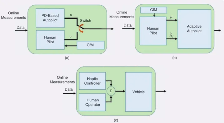
Existing frameworks that combine humans and automa-tion generally rely on human experts supplementing flight control automation, that is, the system is semiautonomous, with the automation handling all uncertainties and distur-bances, with human control occurring once the environment imposes demands that exceed the automation capabilities [1]–[3]. This approach causes bumpy and late transfer of con-trol from the machine to the human (causing the SCA to fail) as it is unable to keep pace with the cascading demand (which may cause actual accidents [4]–[7]). This suggests that alternate architectures of coordination and interaction between the human expert and automation are needed. Var-ious architectures have been proposed in the literature that can be broadly classified into three forms: a trading action, where humans take over control from automation under emergency conditions [8]; a supervisory action, where the pilot assumes a high-level role and provides the inputs and setpoints for the automation to track [9]; and a combined action, where both the automation and the human expert participate at the same timescale [10]. We label all three forms under a collective name of SCA, with SCA1 denoting the trading action, SCA2 the supervisory action, and SCA3 the combined action (see Figure 1 for a schematic of all three forms of SCAs). This article focuses on SCA1 and SCA2 and their validation using human-in-the-loop simulations.
To have an efficient coordination between humans and automation, two principles from cognitive engineering are utilized that study how humans add resilience to complex systems [4], [5], [7]. The first principle is capacity for maneu-ver (CfM), which denotes a system’s reserve capacity that will remain after the occurrence of an anomaly [5]. It is hypothe-sized that resiliency is rooted in and achieved via monitoring and regulation of the system CfM [7]. The notion of CfM exists in an engineering context as well, as the reserve capac-ity of an actuator. Viewing the actuator input power as the system capacity (and noting that a fundamental capacity limit exists in all actuators in the form of magnitude satura-tion), CfM can be defined for an autopilot-controlled system as the distance between the control input and saturation limits. The need to avoid actuator saturation (and, therefore, increasing CfM) becomes even more urgent in the face of anomalies, which may push the actuators to their limits. This implies that there is a common link between pilot-based decision making with an autopilot-pilot-based one in the form of CfM. This commonality is utilized in both SCA1 and SCA2, presented in this article.
The foundations for SCA1 and SCA2 come from the results of [11]–[13], with [11] and [12] corresponding to SCA1 and [13] corresponding to SCA2. In [11], the assumption is that the autopilot is designed to accommodate satisfactory operation under nominal conditions, using the requisite tracking performance. An anomaly is assumed to occur in the form of loss of effectiveness of the actuator (which may be due to damage to the control surfaces caused by a sudden change in environmental conditions or a compromised
Summary
T
his article considers the problem of control when two dis-tinct decision makers, a human operator and an advanced automation working together, face severe uncertainties and anomalies. We focus on shared control architectures (SCAs) that allow an advantageous combination of their abilities and provide a desired resilient performance. Humans and automation are likely to be interchangeable for routine tasks under normal conditions. However, under severe anomalies, the two entities provide complementary actions. It could be argued that human experts excel at cognitive tasks, such as anomaly recognition and estimation, while fast response with reduced latencies may be better accomplished by auto-mation. This then suggests that architectures that combine their action must be explored. One of the major challenges with two decision makers in the loop is bumpy transfer when control responsibility switches between them. We propose the use of a common metric that enables a smooth, bump-less transition when severe anomalies occur. This common metric is termed capacity for maneuver (CfM), which is a concept rooted in human behavior and can be identified in control systems as the actuator’s proximity to its limits of sat-uration. Two different SCAs are presented, both of which use CfM, and describe how human experts and automation can participate in a shared control action and recover gracefully from anomalous situations. Both of the SCAs are validated using human-in-the-loop experiments. The first architecture consists of a traded control action, where the human expert assumes control from automation when the CfM drops below a certain threshold and ensures a bumpless transfer. The second architecture includes a supervisory control action, where the human expert determines the tradeoff between the CfM and the corresponding degradation in command fol-lowing and transmits suitable parameters to the automation when an anomaly occurs. The experimental results show that, in the context of flight control, these SCAs result in a bumpless, resilient performance.engine due to bird strikes). The trading action proposed in [11] is for the pilot to assume control from the autopilot, based on the pilot perception that the automation is unable to address the anomaly. This perception is based on the CfM of the actuator, and when it exceeds a certain threshold, the pilot is proposed to assume control. A well-known model of the pilot in [1]–[3] is utilized to propose the specific sequence of control actions that pilots take once they assume control. It is shown through simulation studies that when the pilot carries out this sequence of perception and control tasks, the effect of anomaly is contained, and the tracking performance is maintained at a satisfactory level. A slight variation of this trading role is reported in [12], where, instead of the “autopi-lot is active → anomaly occurs → pi“autopi-lot control” sequence, the pilot transfers control from one autopilot to a more advanced one following the perception of an anomaly. This article limits attention to the SCA1 architecture in [11] and validates its performance using human-in-the-loop simulations.
The SCA2 architecture utilized in [13] differs from that of SCA1, as mentioned previously, as the trading action from the autopilot to the pilot is replaced by a supervisory action by the pilot. In addition to using CfM, this architecture uti-lizes a second principle from cognitive engineering denoted as graceful command degradation (GCD). GCD is proposed as an inherent metric adopted by humans [4] that will allow the underlying system to function so as to retain a target CfM. As the name connotes, GCD corresponds to the extent
to which the system is allowed to relax its performance goals. When subjected to anomalies, it is reasonable to impose a command degradation; the greater this degradation, the larger the reserves that the system will possess when recov-ered from the anomaly. A GCD can then be viewed as a con-trol variable tuned to permit a system to reach its targeted CfM. The role of tuning this variable so that the desired CfM is retained by the system is relegated to the pilot in [13]. Spe-cifically, a parameter n is transferred to the pilot from the
autopilot, which is shown to result in an ideal tradeoff between the CfM and GCD by the overall closed-loop system with SCA2. This article validates SCA2 using a high-fidelity model of an aircraft and human-in-the-loop simulations.
The subjects used in the human-in-the-loop simulations include an airline pilot (who is also a flight instructor) with 2600 h of flight experience as well as human subjects who were trained in a systematic manner by the experiment designer. The details of the training are explained in the “Validation with Human-in-the-Loop Simulations” sec-tion. It is shown that SCA1 in [11] and SCA2 in [13] lead to better performance, as conjectured therein, when the human expert completes his or her assigned roles in the respective architectures. The resulting solution is an embodiment of an efficient cyberphysical human system, a topic that is of sig-nificant interest of late.
In addition to the aforementioned references, SCAs have been explored in haptic shared control (HSC), which has
Online Measurements Online Measurements Online Measurements Data Data Data PD-Based Autopilot Haptic Controller Human Operator Vehicle Adaptive Autopilot Human Pilot Human Pilot CfM CfM Switch υ υ µ Λ"f Σ (a) (b) (c)
FIGURE 1 An overview of shared control architectures (SCAs). (a) SCA1, in which the autopilot takes care of the control task until an anom-aly, which is then transferred to the pilot based on capacity for maneuver (CfM). (b) SCA2, in which the pilot undertakes a supervisory role. CfM values approaching dangerously small numbers may trigger the pilot to assess the situation and convey necessary auxiliary inputs n
and Kt to the autopilot. (c) SCA3, which is based on the combined control effort continuously transmitted by both the haptic controller and fp human operator, who has the choice of abiding by or dismissing the control support of the automation. PD: proportional derivative.
applications both in the aerospace [14] and automotive [10], [15] domains. In HSC, both the automation and human oper-ator exert forces on a common control interface (such as a steering wheel or a joystick) to achieve their individual goals. In this regard, HSC can be considered to have an SCA3 architecture. In [14], the goal of the haptic feedback is to help an unmanned aerial vehicle operator avoid an obstacle. In [15], one of the goals is lane-keeping, and in [10], the goal is assisting the driver while driving around a curve. All of these approaches provide situational awareness to the human operator, who has the ability to override the haptic feedback by exerting more force to the control interface. An interesting HSC study is presented in [16], where the haptic guidance authority is modified adaptively according to the intensity of the user grip, where challenging scenarios are created by introducing force disturbances or incorrect guid-ance. Another SCA approach is to enable the automation to affect the control input directly instead of using a common interface [17], which can also be viewed as belonging to SCA3. In this approach, the human operator can override the automation by disengaging it from the control system. Since SCA1 and SCA2 architectures help with anomaly mitigation and SCA3 is not shown to be relevant in this respect, this article focuses on SCA1 and SCA2 and their validations using human-in-the-loop simulation studies.
In the specific area of flight control, SCAs have also been proposed for greater situational awareness. A bumpless transfer between the autopilot and pilot is proposed in [18] using a more informative pilot display. It is argued in [18] that a common problem in pilot–automation interaction is the pilot’s unawareness of the automation state and the air-craft during the flight (which makes the automation system opaque to the pilot), prompting the use of such a pilot dis-play. The employment of the display is discussed in [18], in the presence of automation developed in [19] and [20] that provides flight envelope protection with a loss of control logic. A review of recent advances on human–machine inter-action can be found in [21] (where the focus is adaptive auto-mation), in which the automation monitors the human pilot to adjust itself accordingly so as to lead to improved situa-tional awareness. No severe anomalies are considered in [18]–[21], which is the focus of this article. The goal of the SCAs discussed in this article is to lead to a bumpless effi-cient performance in the presence of severe anomalies. Therefore, discussions do not focus on these situational awareness-based research directions.
The following sections introduce the two main compo-nents of SCA: the autopilot and the human pilot. The “Auto-pilot” section provides the details of the employed controllers. The “Human Pilot” section first reviews the main mathemat-ical models of pilots proposed in the literature in the absence of a severe anomaly. The human model used in the develop-ment of the proposed SCAs is then proposed. The working principles of these SCAs are later presented in detail in the section “Shared Control.” Finally, the “Validation with
Human-in-the-Loop Simulations” section shows how the underlying ideas are tested with human subjects.
AUTOPILOT
This section describes the technical details related to the autopilot discussed in [11] and [13].
Dynamic Model of the Aircraft
Since the autopilot in [13] is assumed to be determined using feedback control, the starting point is the description of the aircraft model, which has the form
( ) ( ) ( ) ( ), ( ) ( ), x t Ax t B u t d f x y t Cx t f T K U = + + + = o (1) where x!Rn and u!Rm are deviations around a trim
condition in aircraft states and control input, respectively, d represents uncertainties associated with the trim condi-tion, and UTf x( ) represents higher-order effects due to non-linearities. A is an (n n# ) system matrix and B is an (n m# ) input matrix [both of which are assumed to be known, with
, A B
^ h controllable], and Kf is a diagonal matrix that
reflects a possible actuator anomaly with unknown posi-tive entries mfi. C is a known matrix of size (k n# ), chosen so that y!Rk corresponds to an output vector of interest. It
is assumed that the anomalies occur at time ,ta so that
1
fi
m = for 0#t1ta, and mfi switches to a value that lies between zero and one for t2ta. It is finally postulated that the higher-order effects are such that f x^ h is a known vector that can be determined at each instant of time, while U is an unknown vector parameter. Such a dynamic model is often used in flight control problems [22].
As the focus of this article is the design of a control architecture in the context of anomalies, actuator con-straints are explicitly accommodated. Specifically, assume that u is position/amplitude limited and modeled as
( ) sat ( ) ( ), ( )sgn ( ) , | ( ) | | ( ) | , u t u u tu u t u t u t u t u u t u max max max max max i c c c c c i i i i i i i i i 2 i # = = c ^ m h ) (2)
where umaxi for i=1 f, ,m are the physical amplitude limits of actuator i and ( )u tci are the control inputs to be determined by the SCA. The functions sat $ and ( ) sgn $ ( ) denote saturation and sign functions, respectively.
Advanced Autopilot Based on Adaptive Control
The control input ( )u tci will be constructed using an adap-tive controller. To specify the adapadap-tive controller, a refer-ence model that specifies the commanded behavior from the plant is constructed and of the form [23]
( ) ( ) ( ), ( ) ( ), x t A x t B r t y t Cx t m m m m m m 0 = + = o (3)
where r Rk
0! is a reference input, Am (n n# ) is a Hurwitz
matrix, xm!Rn is the state of the reference model, ^A Bm, mh
is controllable, and C is defined as in (1) (that is, ym!Rk corresponds to a reference model output). The goal of the adaptive autopilot is then to choose ( )u tci in (5), so that if an error, ,e is defined as
( ) ( ) ( ),
e t =x t -x tm (4)
then all signals in the adaptive system remain bounded with error e t^ h tending to zero asymptotically.
The design of adaptive controllers in the presence of control magnitude constraints is first addressed in [24], with guarantees of closed-loop stability through modifica-tion of the error used for the adaptive law. The same prob-lem is addressed in [25] using an approach termed n-mod
adaptive control, where the effect of input saturation is accommodated through the addition of another term in the reference model. Another approach based on a closed-loop reference model (CRM) is derived in [26] and [27] to improve the transient performance of the adaptive controller. The proposed autopilot is based on both the n-mod and CRM
approaches. Using the control input in (2), this controller is compactly summarized as ( ) ( ), ( ) sgn ( ) , || ( ) |( ) | , u t u t u t u t u uu tt uu 11 ad ad ad ad max max max c c i i i i i i i i 2 i # n n = + + d d d ^ ^ h h
*
(5) where ( ) ( ) ( ) ( ) ( ) ( ) ( ) ( ), uadi t =K t x txT +K t r tTr 0 +d tt + tUT t f x (6) ( ) , . udmaxi= 1-d umaxi 0#d11 (7) A buffer region in the control input domain [(1-d)umaxi,]
umaxi is implied by (5) and (7), and the choice of nallows the input to be scaled somewhere in between. The reference model is also modified as
( ) ( ) ( ) ( ) ( ) ( ), x tom =A x tm m +B r tm^ 0 +K t u tTu D ad h-Le t (8) ( ) sat ( ) ( ), uad t umax u tu uad t max c i i i i i D = c m- (9)
and L1 is a constant or a matrix selected such that 0 (Am+L) is Hurwitz. Finally, the adaptive parameters are adjusted as ( ) ( ) ( ) , ( ) ( ) ( ) , ( ) ( ) , ( ) ( ( )) ( ) , ( ) ( ) , K t x t e t PB K t r t e t PB d t e t PB t f x t e t PB K t u e t PBad x x T r r T d T f T u u T m 0 C C C U C C D = = = = -= o o to to o (10)
where P P= T is a solution of the Lyapunov equation (for Q20)
,
A P PAmT + m= -Q (11) with Cx=CxT20,Cr=CrT20,Cu=CTu20.
The stability of the overall adaptive system specified by (1), (2), and (3)–(11) is established in [25] when L=0. The sta-bility of the adaptive system when no saturation inputs are present is also established in [27]. A very straightforward combination of the two proofs can be easily completed to prove that, when L10, the adaptive system in this arti-cle has globally bounded solutions if the plant in (1) is open-loop stable and bounded solutions for an arbitrary plant if all initial conditions and the control parameters in (10) lie in a compact set. The proof is skipped due to page limitations.
The adaptive autopilot in (5)–(11) provides the required control input u in (1) as a solution to the underlying prob-lem. The autopilot includes several free parameters, includ-ing n in (5); d in (7); the reference model para meters Am,
,
Bm and L in (8); and the control parameters Kx( ),0 Kr( ),0
( ),
Ku 0 ( ),dt 0 ( )Ut 0 in (10). As shown in the next section, the parameters d and n are related to CfM and GCD.
Quantification of Capacity for Maneuver and
Graceful Command Degradation and Tradeoffs
The control input uci in (5) is shaped by two parameters, d
and ,n both of which help tune the control input with
respect to its specified magnitude limit, umaxi. These two parameters are used to quantify CfM, GCD, and the trad-eoffs between them as follows.
Capacity for Maneuver
Qualitatively, CfM corresponds to a system’s reserved capacity, which is quantitatively formulated in the current context as the distance between a control input and its satu-ration limits. Specifically, define CfM as
CfM CfM ,CfM d R = (12) where CfM rms ( ( )) | , ( ) | ( ) |, min c t c t umax u t R i i t T i i a i = = -` j (13) where ( )c ti is the instantaneous available control input of
actuator ,i CfMR is the root mean squared CfM variation,
and CfMd (which denotes the desired CfM) is chosen as
CfMd max umax .
i d i
= ^ h (14)
In these equations, min and max are the minimum and maximum operators over the ith index, rms is the root-mean-square operator, and ta and T refer to the time of
anomaly and final simulation time, respectively. From (13), note that CfMR has i) a maximum value u
max for the trivial case when all ( )u ti =0, ii) a value close to ud max if the control inputs approach the buffer region, and iii) a value of
zero if ( )u ti hits the saturation limit umax. Since CfMd=dumax, it follows that CfM (the corresponding normalized value) is greater than unity when the control inputs are small and far away from saturation, unity as they approach the buffer region, and zero when fully saturated.
Graceful Command Degradation
As mentioned earlier, the reference model represents the commanded behavior from the plant being controlled. To reflect the fact that the actual output may be compromised if the input is constrained, a term was added that depends on Du tad( ) in (9) to become nonzero whenever the control input saturates (that is, when the control input approaches the saturation limit, uD adi becomes nonzero), thereby suit-ably allowing a graceful degradation of xm from its
nomi-nal choice, as in (8). This degradation is denoted as GCDi
and quantified as GCD rms(rms( ( ))y ( )r tt r t( )), t T, , , , i i m i i 0 0 0 ! = - (15)
where T0 denotes the interval of interest and ym i, and r0, i indicate the ith elements of the reference model output and reference input vectors, respectively. It should be noted that once n is specified, the adaptive controller automatically
scales the input into the reference model through uD ad and ,
Ku such that e t^ h remains small and the closed-loop system
has bounded solutions.
μ
The intent behind the introduction of the parameter n in
(5) is to regulate the control input and move it away from saturation when needed. For example, if uadi( )t 2umaxd i, the extreme case of n=0 will simply set uci=uad, thereby removing the effect of the virtual limit imposed in (7). As n
increases, the control input would decrease in magnitude and move toward the virtual saturation limit umaxd i, that is, once the buffer d is determined, n controls ( )u ti within the
buffer region [(1-d)umaxi,umaxi], bringing it closer to the lower limit with increasing .n In other words, as n
increases, CfM increases as well in the buffer region. It is easy to see from (8) and (9) that, similar to CfM, as n
increases, GCD also increases. This is because an increase in n increases Duadi( ),t which, in turn, increases the GCD. While a larger CfM improves the responsiveness of the system to future anomalies, a lower bound on the reference command is necessary to finish the mission within practical constraints. In other words, n must be chosen so that GCD
remains above a lower limit while maintaining a large CfM. The task of selecting the appropriate n is relegated to the
human pilot.
Choice of the Reference Model Parameters
In addition to n and ,d the adaptive controller in (2) and
(3)–(11) requires the reference model parameters Am, Bm,
and L and the control parameters Kx( ),0 Kr( ),0 and Ku( )0 at
time t=0. If no anomalies are present, then Knom=Kf= ,I which implies that Am and Bm (as well as the control
parameters) can be chosen as ( ), ( ) ( ) , ( ), ( ) , A A BK K A B B BK K A B 0 0 0 0 m xT r T m m rT u T m 1 1 1 = + = -= = -- -- (16)
where ( )Kx 0 is computed using a linear-quadratic regulator method and the nominal plant parameters ^A B, h [28] and
( )
Kr 0 in (16) are selected to provide unity low-frequency dc gain for the closed-loop system. When anomalies occur (Kf!I) at time t=ta and assuming an estimate Kt is f
available, a choice similar to that in (16) can be completed using the plant parameters ( ,A BKtf) and the relations
( ), ( ) ( ( )) , ( ), ( ) ( ), A A B K t K t A B t B B K t K t A B t m f xT a r T a m f a m f rT a u T a m f a 1 1 1 K K K K = + = -= = -- -t t t t (17)
with the adaptive controller specified using (2)–(11) for all t$ta. Finally, L is chosen as in [27], and lower param-eters ( ), ( )dt 0 Ut 0 are chosen arbitrarily. Similar to ,n the
task of assessing the estimate Kt is also relegated to the fp human pilot.
Autopilot Based on Proportional-Derivative Control
To investigate SCAs, another autopilot employed in the closed-loop system is the proportional-derivative (PD) con-troller. Assuming a single control input [11], the goal is to control the dynamics [1]( ) ( ) , Y sp = s s a1
+ (18)
which represents the aircraft transfer function between the input u and an output M t^ h, which is assumed to be a sim-plified version of the dynamics in (1). The input u is subjected to the same magnitude and rate constraints as those in (2). Considering the transfer function (18) between the input u and output M t^ h, the PD controller can be chosen as
( ) ( ( ) ( )) ( ( )),
u t =K M tp -Mcmd t +K M tr o (19)
where Mcmd is the desired command signal that M is required to follow. Given the second-order structure of the dynamics, it can be shown that suitable gains Kp and Kr
can be determined so that the closed-loop system is stable, and for command inputs at low frequencies, a satisfactory tracking performance can be obtained.
It is noted that, during the experimental validation stud-ies, certain anomalies are introduced to (18) in the form of unmodeled dynamics and time delays. Therefore, accord-ing to the crossover model [29], the human pilots must adapt themselves to demonstrate different compensation
characteristics (such as pure gain, lead, or lag) based on the type of the anomaly. This creates a challenging scenario for the SCA.
HUMAN PILOT
This section discusses mathematical models of human pilot decision making on the basis of the absence and pres-ence of flight anomalies. A great deal of research was con-ducted on mathematical human pilot modeling, assuming that no failure in the aircraft or severe disturbances in the environment are present. Since decision making will differ significantly whether the aircraft is under nominal opera-tion or subjected to severe anomalies, the corresponding models are entirely different as well and discussed sepa-rately in what follows.
Pilot Models in the Absence of Anomaly
In the absence of an anomalous event(s), mathematical models of human pilot control behavior can be classified according to control-theoretic, physiological, and, more recently, machine learning methods [30], [31]. One of the most well-known control-theoretic methods in the model-ing of human pilots (namely, the crossover model) is pre-sented in [29] as an assembly of the pilot and the controlled vehicle for single-loop control systems. The open-loop transfer function for the crossover model is
( ) ( ) , Y j Y jh p cej j e ~ ~ ~ ~ = -x ~ (20)
where ( )Y jh ~ is a transfer function of the human pilot, ( )Y jp ~
is a transfer function of the aircraft, ~cis the crossover
fre-quency, and xe is the effective time delay pertinent to the
system delays and human pilot lags. The crossover model is applicable for a range of frequencies around the crossover frequency .~c When a “remnant” signal is introduced to
( )
Y jh ~ to account for the nonlinear effects of the pilot-vehicle
system, the model is called a quasi-linear model [32].
Other sophisticated quasi-linear models can be found in the literature as the extended crossover model [32] [which works especially for conditionally stable systems, that is, when a pilot attempts to stabilize an unstable trans-fer function of the controlled element, ( )Y jp ~ ] and the
preci-sion model [32] (which treats a wider frequency region than the crossover model). The single-loop control tasks are covered by quasi-linear models. They can be extended to multiloop control tasks by the introduction of the optimal control model [33], [34].
Another approach in modeling the human pilot is employing the information of sensory dynamics relevant to humans to extract the effect of motion, proprioceptive, vestibular, and visual cues on the control effort. An exam-ple of this is the descriptive model [35], in which a series of experiments are conducted to distinguish the influence of vestibular and visual stimuli from the control behav-ior. Another example is the revised structural model [36],
where the human pilot is modeled as the unification of pro-prioceptive, vestibular, and visual feedback paths. It is hypothesized that such cues help alleviate the compensa-tory control action taken by the human pilot.
It is noted that, due to their physical limitations, models such as that in (20) are valid for operation in a predefined boundary or envelope where the environmental factors are steady and stable. In the case of an anomaly, they may not perform as expected [37].
Pilot Models in the Presence of Anomaly
When extreme events and failures occur, human pilots are known to adapt themselves to changing environmental conditions, which overstep the boundaries of automated systems. Since the hallmark of any autonomous system is its ability to self-govern (even under emergency conditions), modeling of the pilot decision making upon the occurrence of an anomaly is indispensable, and examples are present in the literature [1]–[3], [11]–[13], [38], [39]. This article assumes that the anomalies can be modeled either as an abrupt change in the vehicle dynamics [1]–[3], [11], [12], [39] or a loss of control effectiveness in the control input [13], [38]. In either case, the objective is the modeling of the decision making of the pilot so as to elicit a resilient performance from the aircraft and recover rapidly from the impact of the anomaly. Since the focus of this article is shared control, among the pilot models that are developed for anomaly response, we exploit those that explain the pilot behavior in relation to the autopilot. These models are developed using the CfM concept, the details of which are explained in the following sections.
Pilot Models Based on Capacity for Maneuver
A recent method in modeling the human pilot under anomalous events utilizes the CfM concept [11], [13], [38]. As discussed in the “Autopilot” section, CfM refers to the remaining range of the actuators before saturation, which quantifies the available maneuvering capacity of the vehi-cle. It is hypothesized that surveillance and regulation of a system’s available capacity to respond to all events help maintain the resiliency of a system, which is a necessary merit to recover from unexpected and abrupt failures or disturbances [7]. Two different types of pilot models are proposed, both of which use CfM, but in different ways.
Perception Trigger
The pilot model is assumed to assess the CfM and implic-itly compute a perception gain based on it. The quantifica-tion of this gain Kt is predicated on CfMR with the
definition in (13). The perception trigger is associated to the gain ,Kt which is implicitly computed in [11]. The
percep-tion algorithm for the pilot is , , , Kt 01 FF0 11 0 1 $ =) (21)
where
( )[ ( )],
( )
(CfM )
CfM
rms( ( ))
F
G s F t
F t
dt
d
u
u t
3
max p R p R 0 1 m m v n=
=
-=
-
(22) ( )G s1 is a second-order filter introduced as a smoothing and lagging operator into the human perception algorithm, F t^ h is the perception variable,
CfM
Rm is a slightly modified version of CfMR in(13),p
n is the average of (d dt)(CfM )Rm, and vp is the standard deviation of (d dt)(CfM )Rm , both of which are measured over a nominal flight simulation. The computation of these statistical parameters is further elaborated in the “Validation of Shared Control Architec-ture 1” section. The hypothesis is that the human pilot has such a perception trigger ,Kt and when Kt=1, the pilot
assumes control from the autopilot. The “Validation of Shared Control Architecture 1” section validates this per-ception model.
Capacity for Maneuver-Graceful
Command Degradation Tradeoff
The pilot is assumed to implicitly assess the available (nor-malized) CfM when an anomaly occurs and decide on the amount of GCD that is allowable, to let the CfM become com-parable to the CfM .d In other words, assume that the pilot is
capable of assessing the parameter nand input this value to
the autopilot following the occurrence of an anomaly. That is, the pilot model is assumed to take the available CfM as the input and deliver n as the output. The “Validation of Shared
Control Architecture 2” section validates this assessment.
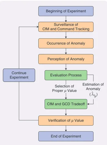
SHARED CONTROL
The focus of this article is on an SCA that combines the deci-sion making of a pilot and autopilot in flight control. The architecture is invoked under alert conditions, with triggers in place that specify when the decision making is transferred from one authority to another. The specific alert conditions of focus in this article correspond to physical anomalies that compromise the actuator effectiveness. The typical roles of the autopilot and pilot in a flight control problem were
Different Forms of Shared Control Architectures
H
uman–machine interactions can be varied in nature, and avast amount of literature of human–machine interactions is available in a number of sectors, including energy, transporta-tion, health care, robotics, and manufacturing. Broadly speak-ing, the resulting systems that emerge from these interactions come under the rubric of the cyberphysical and human system (CPHS).
The adjective shared in the phrase “shared control archi-tectures” (SCAs) is used in a broad sense, where a human ex-pert shares the decision making with automation in some form or the other in the CPHS [S1]. These SCAs can be grouped into three categories: SCA1 as traded [S1], SCA2 as supervised [S2], and SCA3 as combined [S3].
In SCA1, the authority shifts from the automation to the hu-man expert as an emergency override when dictated by the anomaly. For example, in a teleoperation task, if a robot auton-omously travels on the remote environment and at certain time intervals, a human operator assumes control and provides real-time speed and direction commands, and then this type of interaction can be considered traded control.
In SCA2, the human expert is on the loop and provides a supervisory, high-level input to the automation. One such ex-ample may occur in the teleoperation scenario mentioned in the previous paragraph, where the human operator can pro-vide reference points for the mobile robot and the control sys-tem on the robot can autonomously navigate the vehicle, make it avoid obstacles, and reach the reference points.
In SCA3, different from SCA1 and SCA2, the human and the automation are both simultaneously active. For example,
in the discussed teleoperation task, if the human controls the robot via a joystick in real time and, at the same time, the ro-bot controller continuously sends force inputs to the joystick to keep the robot collision-free on the terrain, then this can be considered combined control.
The main distinction between different classifications origi-nates from the timing of the human and automation control in-puts. The commonality between the classes, however, is that both the human and the automation share the load of control, albeit with different timescales. Therefore, for ease of exposi-tion, shared control is used as the collective rubric for both of the interaction types investigated in this article.
It is noted that the use of the adjective shared in this ar-ticle is different than what has been proposed in [S1] and [S2], where the term shared is reserved exclusively for actions that both humans and automation simultaneously exert at the same timescale. We denote this as a combined action (SCA3) and the collective human–automation control architectures as
shared. As we better understand the ramifications of these
dif-ferent types of CPHS, these definitions may also evolve. REFERENCES
[S1] D. A. Abbink et al., “A topology of shared control systems? Finding common ground in diversity,” IEEE Trans. Human-Mach. Syst., vol. 48, no. 5, pp. 509–525, Oct. 2018. doi: 10.1109/THMS.2018.2791570. [S2] T. B. Sheridan, Ed. Monitoring Behavior and Supervisory Control, vol. 1. Berlin: Springer-Verlag, 2013.
[S3] M. Mulder, D. A. Abbink, and E. R. Boer, “Sharing control with hap-tics: Seamless driver support from manual to automatic control,” Hum.
Factors J. Hum. Factors Ergonom. Soc., vol. 54, no. 5, pp. 786–798,
described in the “Autopilot” and “Human Pilot” sections, respectively. In the “Autopilot” section, autopilots based on PD control and adaptive control were described, with the former designed to ensure satisfactory command following under nominal conditions and the latter to accommodate parametric uncertainties (including the loss of control effec-tiveness in the actuators). In the “Pilot Models in the Pres-ence of Anomaly” section, two different models of decision making in pilots were proposed, both based on the monitor-ing of CfM of the actuators. This section proposes two differ-ent SCAs using the models of the autopilots and pilots described in the previous sections (see “Different Forms of Shared Control Architectures”).
Shared Control Architecture 1: A Pilot With a
Capacity for Maneuver-Based Perception and
a Fixed-Gain Autopilot
The first SCA can be summarized as a sequence {autopilot runs, anomaly occurs, pilot takes over}. That is, it is assumed that an autopilot based on PD control [as in (19)] is in place, ensuring satisfactory command tracking under nominal conditions. The human pilot is assumed to consist of a ception component and an adaptation component. The per-ception component consists of monitoring CfMRm, through which a perception trigger F0 is calculated using (22). The adaptation component consists of monitoring the control gain in (21) and assuming control of the aircraft when
.
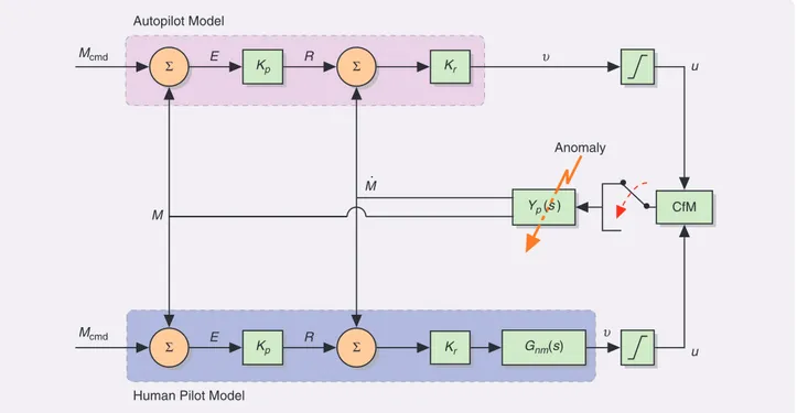
Kt=1 The details of this shared controller and its evalua-tion using a numerical simulaevalua-tion study can be found in [11]. Figure 2 illustrates the schematic of SCA1.
Shared Control Architecture 2: A Pilot With
Capacity for Maneuver-Based Decision Making
and an Advanced Adaptive Autopilot
In this SCA, the role of the pilot is a supervisory one, while the autopilot takes on an increased and more complex role. The pilot is assumed to monitor CfM of the resident actua-tors in the aircraft following an anomaly. In an effort to allow CfM to stay close to CfMd in (14), the command is
allowed to be degraded; the pilot then determines a param-eter n that directly scales the control effort through (5) and
indirectly scales the command signal through (8) and (9). Once n is specified by the pilot, then the adaptive
autopi-lot continues to supply the control input using (5)–(11). If the pilot has high situational awareness, he or she provides
fp
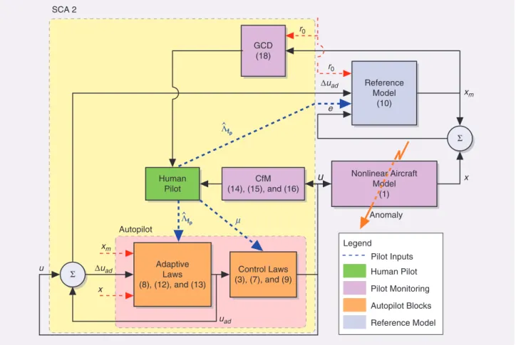
Kt as well, which is an estimate of the severity of the anomaly. The details of this shared controller and its eval-uation using a numerical simulation study can be found in [13] and [38]. Figure 3 displays the schematic of SCA2.
VALIDATION WITH
HUMAN-IN-THE-LOOP SIMULATIONS
The goal in this section is to validate two hypotheses of the human pilot actions, namely, SCA1 and SCA2. Despite the
Σ Kp Kp Kr Kr Σ E R υ υ Σ Gnm(s) E R CfM Yp(s ) • • u M M Autopilot Model
Human Pilot Model
u Mcmd
Mcmd
Anomaly
Σ
FIGURE 2 A block diagram of shared control architecture 1 (adapted from [11]). The autopilot model consists of a fixed gain controller, whereas the human pilot model comprehends a perception part based on the capacity for maneuver (CfM) concept and an adaptation part governed by empirical adaptive laws [3]. The neuromuscular transfer function [42] is Gnm( ),s which corresponds to control input
formed by an arm or leg, Gnm( )s =^100 s2+14 14. s+100h. When an anomaly occurs, the plant dynamics ( )Y sp undergo an abrupt
change by rendering the autopilot insufficient for the rest of the control. At this stage, the occurrence of an anomaly is captured by the CfM such that the control is transferred to the human pilot model for resilient flight control.
presence of obvious common elements to the two SCAs of a human pilot, an autopilot, and a shared controller that com-bines their decision making, the details differ significantly. We therefore describe the validation of these two hypotheses sepa-rately in what follows. In each case, the validation is presented in the following order: the experimental setup, the type of anomaly, the experimental procedure, details of the human subjects, the pilot model parameters, results, and observations.
Although the experimental procedures used for SCA1 validation and SCA2 validation differ (and are therefore explained in separate sections), they use similar principles. To minimize repetition, main tasks can be summarized as fol-lows. The procedure comprises three main phases: Pilot Brief-ing, Preparation Tests, and Performance Tests. In Pilot Briefing, the aim of the experiment and the experimental setup are introduced. In Preparation Tests, the subjects are encouraged to gain practice with the joystick controls. In the last phase, Per-formance Tests, the subjects are expected to conduct the experi-ments only once to not affect the reliability due to learning. Anomaly introduction times are randomized to prevent pre-dictability. As nominal (anomaly-free) plant dynamics, the simpler model introduced in (18) is used for SCA1 validation, and a nonlinear F-16 dynamics [40], [41] is used for SCA2
validation. The experiment was approved by the Bilkent Uni-versity Ethics Committee, and informed consent was taken from each subject before conducting the experiment.
It is noted that during the validation studies, SCA1 and SCA2 are not compared. They are separately validated with different human-in-the-loop simulation settings. However, a comparison of SCA1 and SCA2 can be pursued as a future research direction.
Validation of Shared Control Architecture 1
Experimental Setup
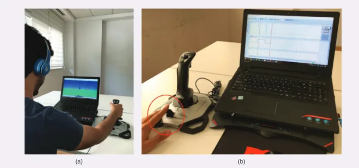
The experimental setup consists of a pilot screen and the commercially available pilot joystick Logitech Extreme 3D Pro (see Figure 4), with the goal of performing a desktop, human-in-the-loop simulation. The flight screen interface for SCA1 can be observed in Figure 4(a) and is separately illustrated in Figure 5. The orange line with a circle in the middle shows the reference to be followed by the pilot. This line is moved up and down according to the desired refer-ence command Mcmd (see Figure 2). The blue sphere in Figure 5 represents the nose tip of the aircraft and is driven by the joystick inputs. When the subject moves the joystick, Human Pilot Adaptive Laws (8), (12), and (13) CfM (14), (15), and (16) GCD (18) Control Laws (3), (7), and (9) Nonlinear Aircraft Model (1) Reference Model (10) Σ Σ xm ∆uad ∆uad xm x u u x uad e r0 r0 µ Anomaly SCA 2 Autopilot Legend Pilot Inputs Human Pilot Pilot Monitoring Autopilot Blocks Reference Model Λfp " Λfp "
FIGURE 3 A block diagram of the proposed shared control architecture 2 (SCA2). The human pilot undertakes a supervisory role by providing the key parameters n and Kt to the adaptive autopilot. The blocks are expressed in different colors based on their functions fp in the proposed SCA2. The numbers in parentheses in each block correspond to the related equations. GCD: graceful command deg-radation; CfM: capacity for maneuver.
he or she provides the control input, ,v which goes through the aircraft model and produces the movement of the blue sphere. The control objective is to keep the blue sphere inside the orange circle, which translates into tracking the reference command. Similarly, the flight screen for SCA2 is seen in Figure 4(b) and separately illustrated in Figure 6. The details on this screen are provided in the “Validation of Shared Control Architecture 2” section.
Anomaly
The anomaly is modeled by a sudden change in vehicle dynamics, from Ybefore( )s
p to Yafterp ( )s (as in [3]), and it is
illus-trated in Figure 2. Two different flight scenarios, Sharsh and Smild, are investigated, which correspond to a harsh and a mild anomaly, respectively. In the harsh anomaly, it is assumed that ( ) ( ) , ( ) ( )( ) , Ybefore, s s s 110 Yafter, s s s e5 s 10 . p h p h s 0 2 = + = + + (23) whereas in the mild anomaly, it is assumed that
( ) ( ) , ( ) ( )( ) . Ybefore, s s s1 7 Yafter, s s s e7 s 9 . p m p m s 0 18 = + = + + (24) The specific numerical values of the parameters in (23) and (24) are chosen so that the pilot action has a distinct effect in the two cases based on their response times. More details of these choices are provided in the following section.
The anomaly is introduced at a certain instant of time ta
in the experiment. The anomaly alert is conveyed as a sound signal at ,ts following which the pilots take over
con-trol at time tTRT, after a certain reaction time tRT. Denoting T ts ta
D = - as the alert time, the total elapsed time from
the onset of anomaly to the instant of hitting the joystick button is defined as
.
tTRT=tRT+DT (25)
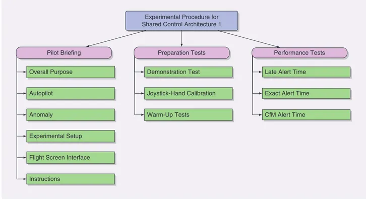
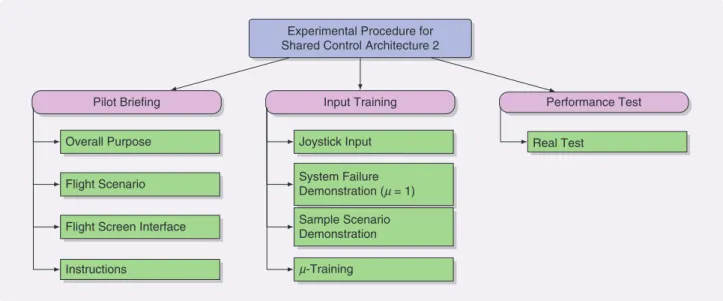
Experimental Procedure
The experimental procedure consists of three main parts: Pilot Briefing, Preparation Tests, and Performance Tests (see Figure 7). The first part of the procedure is the Pilot Briefing, where the subjects are required to read a pilot briefing to have a clear understanding of the experiment. The briefing consists of six main sections: Overall Purpose, Autopilot, Anomaly, Experimental Setup, Flight Screen, and Instructions. In these sections, the main concepts and experimental
(a) (b)
FIGURE 4 The experimental setups for (a) shared control architecture 1 (SCA1) and (b) SCA2. The SCA1 experiment consists of a pilot screen (see Figure 5) and a commercially available pilot joystick, whose pitch input is used. The SCA2 experiment consists of a different pilot screen (see Figure 6) and the joystick. In SCA2, subjects use the joystick lever to provide input.
FIGURE 5 The flight screen interface for shared control architecture 1. The blue sphere represents the aircraft nose and is controlled in the vertical direction via joystick movements. The orange line with a circle in the middle (which also moves in the vertical direction) represents the reference command to be followed. The control objective is to keep the blue sphere inside the orange circle. At the beginning of the experiments, the aircraft is controlled by the auto-pilot. When an anomaly occurs, the subjects are warned to assume control via a sound signal. The time of initiating this signal is determined using different alert times.
hardware (such as the pilot screen and the joystick lever) are introduced to the subject.
The second part is Preparation Tests, in which the subjects are introduced to a demonstration test conducted by the experi-ment designer to familiarize the subjects with the setup. In this test, the subjects observe the experiment designer follow-ing a reference command usfollow-ing the joystick [see Figure 4(a)]. They also watch the designer respond to control switching alert sounds by taking over control via the joystick. Follow-ing these demonstration tests, the subjects are requested to perform the experiment themselves. To complete this part, three preparation tests (each with a duration of 90 s) are con-ducted. At the end of each test, the root mean square error (RMSE) erms of the subjects is calculated as
( ) , erms T1 e d p t T 2 a p x x =
#
(26) where ( ) ( ) ( ) e t =Mcmd t -M t (27) and Tp= .90 s It is expected that the erms in each trial decreases as a sign of learning.The third is the Performance Tests (each with a duration of 180 s), which aim at testing the performance of the proposed SCA in terms of tracking error erms, CfMRm, and a bumpless transfer metric t(which is calculated using the difference
between erms values that are obtained using the 10-s inter-vals before and after the anomaly). This calculation is per-formed as ( ) ( ) . ta 110 t e d t1 e d t a t t 10 2 10 2 a a a a t= x x x x + -+
-#
#
(28)Details of the Human Subjects
The experiment with the harsh anomaly was conducted by 15 subjects (including one flight pilot), whereas the one with the mild anomaly was conducted by three subjects (including one flight pilot). All subjects were more than 18 years old, and four of the subjects were left-handed. However, this did not bring about any problems since an ambidextrous joystick was utilized. Some statis-tical data pertaining to the subjects are given in Table 1.
Pilot Model Parameters
The pilot model in (21)–(22) includes statistical parame-ters np and ,vp the mean and the standard deviation
0 5 10 15 20 1 0.8 0.6 0.4 0.2 100 –100 0.01 0.005 0 0 0 25 30 35 40 45 50 55 60 65 70 75 80 85 90 95 100 105 110 115 120 0 5 10 15 20 25 30 35 40 45 50 55 60 65 70 75 80 85 90 95 100 105 110 115 120 CfM
Reference Altitude (r0) Actual Altitude
GCD Antilocking Range [0–20] 13 (a) (b) (c)
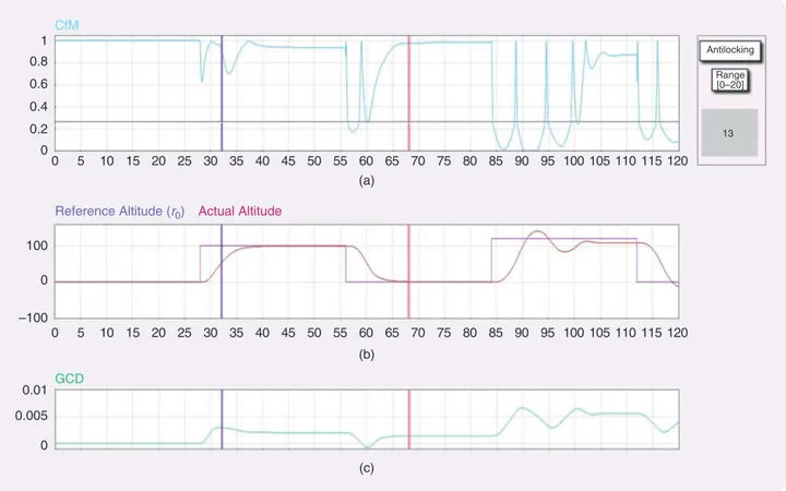
FIGURE 6 The flight screen interface for shared control architecture 2. Part (a) shows the normalized ( )c ti in (13), which can be
consid-ered as the instantaneous capacity for maneuver (CfM). The purple- and maroon-colored vertical lines at ta1=32 s and ta2=68 s, respectively, show the instants of anomaly introduction. The horizontal black line is the antilocking border, below which the n input becomes effective. It is explained to the subjects as well as demonstrated during training that setting n to high values where CfM tion is over this border has no influence on CfM [which is apparent from (5)]. Part (b) shows reference tracking, and (c) is the time varia-tion of the graceful command degradavaria-tion during flight. GCD: graceful command degradavaria-tion.
of the time derivative of CfMRm, respectively, and the parameters of the filter G s1( ). The filter is chosen as
( ) . . .
G s1 =^2 25 s2+1 5s+2 25h to reflect the bandwidth of the pilot stick motion. To obtain the other statistical parameters, several flight simulations were run with the PD control-based autopilot in closed loop, and the resulting CfMRm values were calculated for 180 s, both for the harsh and mild anomalies. The time-averaged statistics of the resulting profiles were used to calculate the statistical parameters as np=0 028. ,vp=0 038. for the harsh anomaly and np=0 091. ,vp=0 077. for the mild anomaly.
The pilot model in (21)–(22) implies that the pilot per-ceives the presence of the anomaly at the time instant when Kt becomes unity, following which the control
action switches from the autopilot to the human pilot. The action of the pilot, based on this trigger, is intro-duced in the experiment by choosing ts (the instant of
the sound signal) to coincide with the perception trig-ger. The corresponding D =T ts-ta, where ta is the
instant when the anomaly is introduced, is denoted as CfM based. To benchmark this CfM-based switching action, two other switching mechanisms are introduced, one defined to be “exact” (where ts=ta, so that TD =0) and another to be “late” (where TD is chosen to be sig-nificantly larger than the CfM-based one). These choices are summarized in Table 2.
Overall Purpose Autopilot Anomaly
Experimental Setup Flight Screen Interface Instructions
Demonstration Test Joystick-Hand Calibration Warm-Up Tests
Late Alert Time Exact Alert Time CfM Alert Time Experimental Procedure for
Shared Control Architecture 1
Pilot Briefing Preparation Tests Performance Tests
FIGURE 7 The experimental procedure breakdown for shared control architecture 1. Three main tasks constituting the procedure are shown. In Pilot Briefing, the subjects read the pilot briefing, review it with the experiment designer, and have a question and answer session. In Preparation Tests, the subjects become familiar with the test via demonstration runs and warm-up tests. Finally, in
Perfor-mance Tests, the real tests are conducted using three different alert times. CfM: capacity for maneuver.
Scenario Number of Participants Female n(Age) v(Age)
Left-Handed
Sharsh 15 1 22.9 3.6 3
Smild 3 0 26.0 5.2 0
TABLE 1 The statistical data of the subjects in the shared control architecture 1 experiment. n() and v() represent the average and the standard deviation operators, respectively.
Switch ta(S) ts(S) DT(S)
Scenario with the harsh anomaly, Sharsh.
Late 50 55.5 5.5
Exact 50 50 0
CfM based 50 51.1 1.1
Scenario with the mild anomaly, Smild.
Late 64 74 10
Exact 64 64 0
CfM based 64 70.2 6.2
TABLE 2 The timeline of anomalies. Based on the switching mechanism, the anomaly is reported to the subject with a sound signal at ts. DT, the alert time, is defined as the time elapsed between the sound signal and the occurrence of the anomaly. CfM: capacity for maneuver.
Results and Observations
Scenario 1: Harsh Anomaly
The results related to the harsh anomaly defined in (23) are presented for various alert times transmitted to the subjects. To compare the results obtained from the subjects, numerical simulation results are completed, where the participants are replaced with the pilot model (21)–(22) using the same alert times. The results obtained are summarized in Table 3 using both the tracking error erms and the corresponding CfMRm.
All numbers reported in Table 3 are averaged over all 15 subjects. erms (scaled by 104) was calculated using (26) with Tp=180 s, while CfMRm wascalculated using (22) with
.
umax=10 The statistical variations of both erms andCfMRm over the 15 subjects are quantified for all three SCA experi-ments. The late, exact, and CfM-based alert times are summa-rized in Table 4. The average bumpless transfer metric t and
its standard error vM( )t are also determined for these three
cases in Table 5. Table 5 also provides the average reaction times tRT and average total reaction times tTRT of the subjects.
Observations
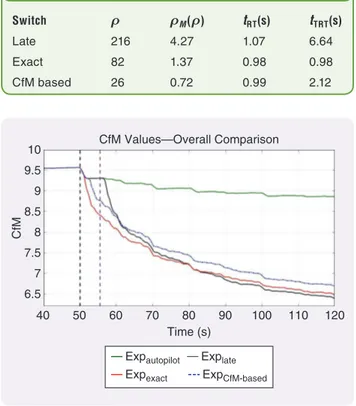
The first observation from Table 3 is that the erms for the CfM-based case is at least 25% smaller than that for the case with the autopilot alone. The second observation is that, among the SCA experiments, the one with the CfM-based alert time has the smallest tracking error, while the one with the late alert time has the largest tracking error. How-ever, it is noted that the difference between the exact and CfM-based cases is not significant.
The third observation from Table 3 is that CfM-based control switching from the autopilot to the pilot provides not only the smallest tracking error but also the largest CfMRm value compared to other switching strategies. This can also be observed in Figure 8, where CfMRm values (averaged over all subjects) are provided for different alert times. As noted earlier, the large CfMRm value of the autopilot results from inefficient use of the actuators, which manifests itself with a large tracking error. The final observation (which comes from Table 5) is that among different alert times, the CfM-based alert time provides the smoothest transfer of control (with a bumpless transfer metric of t = 26), while the late
alert provides t = 216 and the exact alert gives t = 82.
These observations imply the following. The pilot reen-gagement after an anomaly should not be delayed until it
Sharsh Auto Simlate Explate Simexact Expexact SimCfM-based ExpCfM-based
erms 478 363 383 319 354 318 348
CfMRm 8.92 7.93 6.84 7.83 6.80 7.83 7.06
TABLE 3 The averaged erms and capacity for maneuver (CfMRM) values for Sharsh. “Sim” refers to simulation, and “Exp” refers to experiment. The autopilot shows the worst tracking error performance. The reason for a high CfMRM amount for the autopilot is the inability to effectively use the actuators to accommodate the anomaly.
Experiment n vM Experiment n vM
Explate 383 16 Explate 6.84 0.10
Expexact 354 15 Expexact 6.80 0.12
ExpCfM-based 348 14 ExpCfM-based 7.06 0.11
TABLE 4 Mean, n, and standard error, vM=v/ n, where
v is standard deviation and n is the subject size of erms (on
the left) and capacity for maneuver (CfMRM) (on the right) for a harsh anomaly.
Switch t tM(t) tRT(s) tTRT(s)
Late 216 4.27 1.07 6.64
Exact 82 1.37 0.98 0.98
CfM based 26 0.72 0.99 2.12
TABLE 5 The averaged bumpless transfer metric t and standard error vM( )t =v t( )/ n, where v is the standard deviation of t,n is the subject size, averaged reaction times is tRT, and total reaction times is tTRT for Sharsh. The least amount
of bumpless transfer of control is in the case of capacity for maneuver (CfM)-based shared control architecture.
10 9.5 9 8.5 8 7.5 7 6.5 CfM 40 50 60 70 80 90 100 110 120 Time (s) Expautopilot
Expexact ExpCfM-based
Explate
CfM Values—Overall Comparison
FIGURE 8 The capacity for maneuver (CfMRm) variation for the autopilot and all of the alert timing mechanisms. CfMRms of Exp
late
and Expexact show changing trends during the simulation.
How-ever, CfMRm of Exp
CfM based- prominently stays at the top, especially
becomes too late, which corresponds to a late-alert switching strategy. At the same time, immediate pilot action right after the anomaly detection might not be necessary either, which is indicated by the fact that the bumpless transfer metric and the CfMRm values for the CfM-based switching case is better than the exact-switching case. Instead, moni-toring the CfMRm information carefully may be the appro-priate trigger for the pilot to assume control.
Scenario 2: Mild Anomaly
The averaged erms (scaled by 104) and CfMRm values for this case are given in Table 6. The averaged bumpless transfer metric ,t its standard error vM( ),t the average reaction
times tRT, and the average total reaction times tTRT are pre-sented in Table 7. The statistical variations of these metrics over the three subjects are depicted in Table 8.
Observations
Similar to the harsh anomaly case, pure autopilot control results in the largest tracking error in the case of a mild anom-aly. Also similar to the harsh anomaly case, pilot engage-ment based on CfMRm information produces the smallest tracking error (although the difference between the exact switching and CfM-based switching is not significant). However, in terms of preserving CfMRm, Table 8 demon-strates that no significant differences between different switching times can be detected due to the wide spread (high standard error) of the results. The same conclusion can be drawn for the bumpless transfer metric. One reason for this could be the low sample size (three) in this experi-ment. One conclusion that can be drawn from these results is that although CfM-based switching shows smaller track-ing errors (compared to the alternatives), the advantage of the proposed SCA in the presence of mild anomaly is not as prominent as in the case of harsh anomaly.
Validation of Shared Control Architecture 2
Unlike SCA1 (where the pilot took over control from the autopilot when an anomaly occurred), in SCA2, the pilot plays more of an advisory role, directing the autopilot that remains operational throughout. Specifically, the pilot pro-vides appropriate values nand, sometimes, Ktfp.
Experimental Setup
Contrary to the SCA1 case, the subjects use the joystick only to enter the n and Kt values using the joystick lever. The fp
flight screen that the subjects see is illustrated in Figure 6. There are three subplots, which are normalized
c t
i( )
(a),reference command ( )r0 tracking (b), and the evolution of GCD (c). The horizontal black line in the normalized
c t
i( )
subplot corresponds to the upper bound of the virtual buffer [ , ]0 d =[ , . ].0 0 25 The small rectangle in the upper right shows the amount of the n input entered via the
joy-stick lever. In this rectangle, the title “Antilocking” is used to emphasize the purpose of the n input, which is
prevent-ing the saturation/lockprevent-ing of the actuators. There is also another region in this rectangle called the “Range,” which shows the limits of this input. The snapshot of the pilot screen in Figure 6 displays a scenario with two anomalies introduced at ta1=32 s and ta2=68 s. The instants of
anomaly occurrences are marked with vertical lines, the colors of which indicate the severity of the anomaly. The subjects are trained to understand and respond to the severity and the effect of the anomalies by monitor-ing the colors, CfM information, and trackmonitor-ing performance.
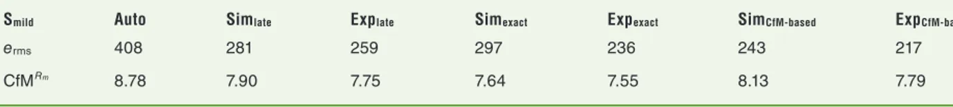
Smild Auto Simlate Explate Simexact Expexact SimCfM-based ExpCfM-based
erms 408 281 259 297 236 243 217
CfMRm 8.78 7.90 7.75 7.64 7.55 8.13 7.79
TABLE 6 The averaged erms and capacity for maneuver (CfMRM) values for Smild. The autopilot still shows the worst performance.
However, the error introduced is less than that of the harsh anomaly.
Switch t tM(t) tRT(s) tTRT(s)
Late 196 3.23 1.06 11.06
Exact 209 8.88 1.02 1.02
CfM based 203 2.87 0.95 7.20
TABLE 7 The averaged bumpless transfer metric t; standard error vM( )t =v t( )/ n, where v is standard deviation of t and n is the subject size; averaged reaction time tRT; and total
reaction time tTRT for the experiment with a mild anomaly Smild.
The nature of the anomaly has a considerable effect on the bumpless transfer metric, that is, the difference between the exact and capacity for maneuver (CfM)-based alert timings is not as readily noticeable as the one of the harsh anomaly.
Experiment n vM Experiment n vM
Explate 259 19 Explate 7.75 0.15
Expexact 236 21 Expexact 7.55 0.17
ExpCfM-based 218 14 ExpCfM-based 7.61 0.19
TABLE 8 The mean n, and standard error vM=v/ n, where v is the standard deviation and n is the subject size of erms (on the left) and capacity for maneuver (CfMRM) (on