Pole assignment problem: A structural investigation

Pole assignment problem: a structural investigation

AYLA SEFIKH and M. EROL SEZERt

Based on the structure of a closed-loop system under a specified feedback pattern, a qualitative analysis of the problem of pole assignability is considered. The problem is first formulated algebraically, in terms of the relation p = g(f) between the vector p of the closed-loop characteristic polynomial coefficients and the vector

f

of the non-zero elements of the feedback matrix. Then, translation to the structural framework is achieved by means of two theorems which give graph-the-oretical sufficient conditions for solvability. These structural conditions also guarantee genericity of pole assignability.

I. Introduction

In the analysis of dynamical systems, such features as high dimensionality, uncertainty in system parameters, and constraints on information structure often lead to complications which cannot be solved by traditional methods. On the other hand, it may be possible to establish a way out through such problems after gaining sufficient insight into the structure of the system. This need for dealing with system structures is met by a qualitative analysis based on the structure of the system (structural analysis). This type of analysis is concerned with general properties of systems such as controllability, observability, existence of fixed modes, etc., which may also be regarded as the potential system properties. This is consistent with physical reality since system parameter values are never known precisely. The fact that digital computers work with true zeros and fuzzy numbers is another justifica-tion for this approach. Investigajustifica-tion of these properties from the genericity point of view is also of interest. A system is said to possess a property generically if that property holds for almost all values of the non-zero system parameters. In other words, if a property of a system is generic, then it fails to hold only in pathological cases when there is an exact matching of system parameters.

It was Lin (1974) who first introduced the concept in his characterization of structural controllability for single-input systems. His result was extended to the multi-input case by Shields and Pearson (1976). Sezer and Siljak ( 1981) developed their characterization for structurally fixed modes in the same context.

This paper is concerned with a structural analysis of the problem of pole assignability. Non-zero system parameters are assumed to be algebraically indepen-dent and structural modelling based on structured matrices and directed graphs (digraphs) is used for system discription. Graph-theoretic formulations due to Reinschke ( 1984) serve as tools in constructing our main results, which give graphical sufficient conditions for generic pole assignability by constant output feedback.

Section 2 is devoted to the formulation of the problem both algebraically and generically together with the establishment of the framework necessary for our

Received 15 May 1989. Revised 24 February 1991. t Bilkent University, 06533 Bilkent, Ankara, Turkey.

tAt present with Eastern Mediterranean University, North Cyprus. 0020-7179/91 $3.00 © 1991 Taylor & Francis Ltd

Pole assignment problem: a structural investigation

AYLA SEFIKTI and M. EROL SEZERT

Based on the structure of a closed~loop system under a specified feedback pattern, a qualitative analysis of the problem of pole assignability is considered. The problem isfirst formulated algebraically, in terms of the relation p = g( f) between the vector p of the closed-loop characteristic polynomial coefficients and the vector f of the non-zero elements of the feedback matrix. Then, translation to the

structural framework is achieved by means of two theorems which give

graph-the-oretical sufficient conditions for solvability. These structural conditions also guarantee genericity of pole assignability.

1. Introduction

In the analysis of dynamical systems, such features as high dimensionality, uncertainty in system parameters, and constraints on information structure often

lead to complications which cannot be solved by traditional methods. On the other

hand, it may be possible to establish a way out through such problems after gaining sufficient insight into the structure of the system. This need for dealing with system structures is met by a qualitative analysis based on the structure of the system (structural analysis). This type of analysis is concerned with general properties of systems such as controllability, observability, existence offixed modes, etc., which may also be regarded as the potential system properties. This is consistent with physical reality since system parameter values are never known precisely. The fact that digital computers work with true zeros and fuzzy numbers is another justifica~ tion for this approach. Investigation of these pr0perties from the genericity point of view is also of interest. A system is said to possess a property generically if that

property holds for almost all values of the non-zero system parameters. In other

words, if a property of a system is generic, then it fails to hold only in pathological cases when there is an exact matching of system parameters.

It was Lin (1974) who first introduced the concept in his characterization of structural controllability for single-input systems. His result was extended to the multi-input case by Shields and Pearson (1976). Sezer and Siljak (1981) developed their characterization for structurally fixed modes in the same context.

This paper is concerned with a structural analysis of the problem of pole

assignability. Non-zero system parameters are assumed to be algebraically

indepen-dent and structural modelling based on structured matrices and directed graphs (digraphs) is used for system discription. Graph-theoretic formulations due to Reinschke (1984) serve as tools in constructing our main results, which give graphical sufficient conditions for generic pole assignability by constant output feedback.

Section 2 is devoted to the formulation of the problem both algebraically and generically together with the establishment of the framework necessary for our

Received 15 May 1989. Revised 24 February 1991. TBilkent University, 06533 Bilkent, Ankara, Turkey.

1 At present with Eastern Mediterranean University, North Cyprus. 0020-7179/91 $3.00 © I99! Taylor & Francis Ltd

974 A. Sefik and M. E. Sezer

structural approach. In § 3, we state and prove the two main theorems of the paper. Section 4 includes examples of classes of generically pole assignable systems that satisfy these results, thus demonstrating their non-triviality. A search algorithm to check the existence of a constant output feedback matrix which satisfies the conditions of the theorems is given in the Appendix.

2. Problem formulation and preliminaries

2.1. Algebraic formulation of the pole assignment problem

Consider a linear, time-invariant system described as Y': :.i:=Ax+Bu}

y=Cx (I)

where x(t) e 11\l", u(t) e 11\lm and y(t) e llil' are the state, input and output of Y', and

A, Band Care real constant matrices of appropriate dimensions.

Let F be an m x r matrix with v :,;; mr non-zero elements which can be chosen arbitrarily. Applying a constant output feedback

.f/': u

=

Fy

to Y' in (I) results in a closed-loop system

Y'(.f/'): :.i: =(A+ BFC)x

having a characteristic polynomial

p(s)

=

det (sf -A - BFC)

=s"+p,sn-1

+ ...

+Pn-IS +Pn

(2)

(3)

(4) Let the non-zero, arbitrary elements of F be represented as a point

f

= (

f

_{1 , /}2 , .•• , / , ) in 11\l', and the coefficients of the characteristic polynomial p(s) in

( 4) as a point p = ( _{p 1, p}2 , ••• , Pn) in 11\l". Then, the relation between p and f can be

represented by a smooth mapping g : 11\l'--. 1\J as

p =g(f) (5)

where 1\J is a smooth manifold in 11\l". The pole-assignment problem is concerned with the existence of a solution

f

e 11\l' of (5) for every given p e 11\l".

We observe that v ~ n is a necessary condition for solvability of (5) for all p,

which we assume to hold in the rest of the paper. Let us, then, partition the feedback variables f, ,/_{2 , ••• , / ,} into two disjoint subsets of fv and fc, respectively. Fixing the varaibles in

fc

at particular real values, ( 5) is reduced to

p =g(f,) (6)

where

g:

11\l"--. 11\l" is a restriction of g to 11\l". The following result (Reinschke 1987) gives a sufficient condition for pole assignability.

Lemma I

Assume n :,;; v :,;; mr. If there exists a partitiOning of the feedback variables

f

1,f2 , ••• ,/,into two disjoint setsfv andfc containing nand v -n elements such that

974 A. Sefik and M. E. Sezer

structural approach. In § 3, we state and prove the two main theorems of the paper. Section 4 includes examples of classes of generically pole assignable systems that satisfy these results, thus demonstrating their non-triviality. A search algorithm to check the existence of a constant output feedback matrix which satisfies the conditions of the theorems is given in the Appendix.

2. Problem formulation and preliminaries

2.l. Algebraic formulation of the pole assignment problem

Consider a linear, time-invariant system described 'as

y; x—Ax+Bu} (l)

y = Cx

where x(t) e R", u(t) e [Rm and y(t) 6 IR’ are the state, input and output of 5”, and A, B and C are real constant matrices of appropriate dimensions.

Let F be an m x r matrix with v S mr non-zero elements which can be chosen arbitrarily. Applying a constant output feedback

9": u = Fy (2)

to y in (1) results in a closed-loop system

54%”): 5c=(A +BFC)x (3)

having a characteristic polynomial

p(s) = det (sl — A — BFC)

=s"+p.s”"+"'+p,._.s+p,. (4)

Let the non-zero, arbitrary elements of F be represented as a point [a (f, ,fz, ...,fv) in R“, and the coefficients of the characteristic polynomial [1(5) in

(4) as a point p = (pbpz, ...,p,,) in R". Then, the relation between p and foam be

represented by a smooth mapping g : W» N as

p=g(f) (5)

where N is a smooth manifold in R". The pole—assignment problem is concerned with the existence of a solution fe R” of (5) for every given p E R".

We observe that v 2n is a necessary condition for solvability of (5) for all p, which we assume to hold in the rest of the paper. Let us, then, partition the feedback variables fhfz, ...,fl into two disjoint subsets offV and fc, respectively. Fixing the varaibles in f; at particular real values, (5) is reduced to

P =§(fu)

(6)

where g' : W—r R" is a restriction of g to IR". The following result (Reinschke 1987) gives a sufficient condition for pole assignability.

Lemma 1

Assume n S. v S mr. If there exists a partitioning of the feedback variables fufz, ...,fi into two disjoint sets fV andfc containing n and v — n elements such that

after appropriately fixing those in fc the derivative

if,

is unimodular, then the system Y' is arbitrarily pole assignable by' the feedback ff. D Note that when

if,

is unimodular, then del if, is a constant so that

i

is a homeomorphism; that is, for every p E ~", there exists a unique

f.

E ~" satisfying

i(/.) = g(f.,fc) = p.

Our main concern is this paper lies in a qualitative analysis of the pole assignment problem, based on the structure of the pair ( !/', ff). In particular, we aim at deriving a structural counterpart of Lemma I, and providing graph-theoretic conditions for generic pole assignability. We devote the rest of this section to establishing the framework needed for this approach.

2.2. Structural representation of systems

In this section, we review some basic concepts and results related to structured matrices, genericity (Shields and Pearson 1976), graph theory ( Harary et a/. 1965), and structural representation of systems (Sage 1977).

Structured matrices and generic properties

Two matrices M,, M₂ E W x • are said to be 'structurally equivalent' if there is

one-to-one correspondence between the locations of their non-zero entries. The equivalence class of structurally equivalent matrices in W x • can be represented by

a p x q 'structured matrix' M, whose entries are either fixed zeros or algebraically independent parameters in R If M has Jl non-zero parameters, then associated with M we define a parameter space ~" such that for every dE~". M(d) defines a fixed matrix in the equivalence class that M represents. A fixed matrix M is said to be admissible with respect to M, denoted as ME M, if M = M(d) for some dEW.

Let IT be a property asserted about the structured matrix M. Then it is a mapping IT:~" .... {0, I} defined as

IT(d)

={I,

if IT h~lds for M(d) 0, otherwise

Let <I>( d) be a polynomial in d = (d1, ••• , d") with real coefficients. The set

r=

{dE~" 1 <I>(d)

=0}

is a 'variety' in ~".

r

is said to be proper if

r

of.~" and non-trivial if

r

of.

0.

The property IT is said to be 'generic' if there exists a proper variety

r

such that ker IT c:

r.

A generic property holds almost everywhere in W.

The 'generic rank' of a structured matrix M, denoted by p( M), is the maximal rank M(d) can achieve ford E ~". The set {dE~"

I

rank M(d) < p(M)} can easily be shown to be a proper variety in ~", so that almost all fixed matrices M(d) have rank p(M).

Diagraphs

A 'diagraph' is an ordered pair [f)= ( f , 8), where f is a finite set of 'vertices' and S a set of oriented 'edges'. An edge oriented from vj E f to v, E f is denoted by the ordered pair (vj, v1 ), where vj is called the 'tail' and v, the 'head' of the edge.

If (vj, v1) E S, then vj is said to be 'adjacent' to v,, and v, adjacent from vj. The

after appropriately fixing those in fc the derivative gfv is unimodular, then the System 5” is arbitrarily pole assignable by' the feedback .97. [Z] Note that when gfv is unimodular, then det gfv is a constant so that g is a homeomorphism; that is, for every p e R”, there exists a unique fv 6 IR" satisfying

EU?) =g(fv,fc)

=11-Our main concern is this paper lies in a qualitative analysis of the pole assignment problem, based on the structure of the pair (9’, 97). In particular, we aim at deriving a structural counterpart of Lemma I, and providing graph-theoretic conditions for generic pole assignability. We devote the rest of this section to establishing the framework needed for this approach.

2.2. Structural representation of systems

In this section, we review some basic concepts and results related to structured

matrices, genericity (Shields and Pearson 1976), graph theory (Harary et 01. I965), and structural representation of systems (Sage 1977).

Structured matrices and generic properties

Two matrices M 1, M2 6 W” are said to be ‘structurally equivalent’ if there is one—to-one correspondence between the locations of their non-zero entries. The equivalence class of structurally equivalent matrices in R” X" can be represented by a p x q ‘structured matrix’ M, whose entries are either fixed zeros or algebraically independent parameters in IR. If M has it non-zero parameters, then associated with M we define a parameter space R” such that for every d e R”, M(d) defines a fixed matrix in the equivalence class that M represents. A fixed matrix M is said to be admissible with respect to M, denoted as M e M, if M = M(d) for some d e R“.

Let H be a property asserted about the structured matrix M. Then it is a

mapping IT : lR“—>{O, 1} defined as

I, if H holds for M(d)

0, otherwise

H(d) = {

Let <b(d) be a polynomial in d =(dl, ..., d“) with real coefficients. The set I‘={delR“|(D(d) =0}

is a ‘variety’ in R”. F is said to be proper if F 7‘5 R“ and non-trivial if F #5 Q. The property [I is said to be ‘generic’ if there exists a proper variety F such that ker 11 c l". A generic property holds almost everywhere in IR”.

The ‘generic rank’ of a structured matrix M, denoted by fi( M), is the maximal rank M(d) can achieve for d 6 IR”. The set {d e R“ I rank M(d) <fi(M)} can easily be shown to be a proper variety in R“, so that almost all fixed matrices M(d) have rank p'(M).

Diagraphs

A ‘diagraph’ is an ordered pair .02 = (V, a“), where ‘V is a finite set of ‘vertices’ and ct? a set of oriented ‘edges’. An edge oriented from v,» e V to v, e "V is denoted by the ordered pair (0], v,), where vj is called the ‘tail’ and v, the ‘head’ of the edge. If (vj, 1),) 66", then 0] is said to be ‘adjacent’ to 1);, and 1),- adjacent from v]. The

976 A. !)efik and M. E. Sezer

adjacency relation can be described by a square binary matrix, R = ( rij) such that rij

=

_{1 if and only if(v1, v}1 ) E c!. A sequence of edges {(v" v2), (v2, v3), ... , (vk-~> vd}

where all vertices are distinct is called a 'path' from v, to v., denoted by (v1 , v.). In

this case, v. is said to be 'reachable' from v,. If v• coincides with v1 , then the path is called a 'cycle'. The path that remains after the removal of an edge of a cycle is called the 'complementary path' of that edge relative to the cycle. Any two cycles are said to be 'disjoint' if they have no common vertices. A collection of disjoint cycles is called a 'cycle family'.

A diagraph §J,

= (

"Y, <!,), with a vertex set "Y,

= {

v_{0 ,} v,, ... , V1 } and an edge set d, = _{{(v0, v1 ), (v,, v2), ... , (v}1 _ 1 , V1 ) } , is called a 'stem'. v0 and V1 are the 'origin' and

the 'tip' of the stem, respectively. A digraph §Jb

=

("Y, <!b), with "Y as above and

db=S_,.u{(v0 v1) } is called a 'bud'. v0 is the origin and (v0,v.) is called the

'distinguished edge' of §Jb· A cactus is a digraph §Jc = §3, _{u Db, u§Jb2, ... , u} Dbk>

where §J, is a stem with origin v0 and tip v,; and §Jb, are buds with origins v, # V1

such that v1 is the only vertex common to E0,u§Jb1 u§Jb2u ... u§Jb_1 _ 1 and §Jb,, i

=

I, ... , k. Origin v0 and tip v1 of §J, are also the origin and the tip of §Jc, respectively.

If §J, above is replaced by a bud, then the digraph is called a 'precactus', denoted

by §Jr. Clearly, by deleting an appropriate edge of a precactus, it can be reduced to

a cactus.

In a cactus, every vertex is reachable from the origin through a unique path. If in a cactus §Jc = ("Yc, Sc), vertices that are adjacent from the origin v0 are

v,, v2 , ... , v., then the sets '"f/"1

= {

v E "Y

I

v is reachable from v1 } are disjoint and

'"f/"c = { v0} u "Y 1 u "Y2 u ... u "Y •. Each of the subgraphs of §Jc defined by one of the

vertex sets {v0 } u '"lr, is called a 'bunch' of the cactus. The bunch that contains the

tip of the cactus is called the 'terminal bunch', and the others (if any) 'non-terminal bunches'. Thus a terminal bunch is a cactus itself and a non-terminal bunch is a precactus.

System structure matrix and system digraph

Associated with the system Y' of (I), we define a square structured matrix as

[

A B 0]

S= 0 0 0

c

0 0

(7)

which is called the 'system structure matrix'. Viewing the matrix S as a binary matrix with zero and non-zero elements, we define the digraph §J =

c·r,

S) which assumes S as its adjacency matrix to be the digraph of the system Y'. For convenience, the

vertex set of§} can be partitioned as "Y

=

11/iuf!lu'f//, where IJ/1, f!l and 'f/1 are the sets of input, state and output variables, respectively. The system diagraph §}completely characterizes the structure of Y'. We say that two dynamic systems are structurally

equivalent if their digraphs are the same up to an enumeration of 1111, f!l and 'f/1.

The subgraph Dux= (f!lulf/1, Su.J obtained by removing from §J the output vertices and the edges connected to them is called the input-truncated system digraph and corresponds to the system structure matrix

(8)

976 A. Sefik and M. E. Sezer

adjacency relation can be described by a square binary matrix, R = (rij) such that

rij = l ifand only if (of, 0,) E (3’. A sequence of edges {(vI , v2), (122, 03), ..., (uh I , vk)}

where all vertices are distinct is called a ‘path’ from v, to uk, denoted by (vl , 0,.) In this case, 1),, is said to be ‘reachable’ from v], 1ft),r coincides with 0., then the path

is called a ‘cycle’. The path that remains after the removal of an edge of a cycle is

called the ‘complementary path’ of that edge relative to the cycle. Any two cycles are said to be ‘disjoint’ if they have no common vertices. A collection of disjoint cycles is called a ‘cycle family’.

A diagraph 95 = (“t/s, 6’5), with a vertex set “Vs = {00, 0., ..., 0,} and an edge set

6,. = {(00, 1).), (0., v2), (v,_,, v,)}, is called a ‘stem’. v0 and v, are the ‘origin’ and

the ‘tip’ of the stem, respectively. A digraph 9b: (V, 63,), with “I” as above and 6b = (3",. u{(v,, 0.)} is called a ‘bud’. 00 is the origin and (120, u.) is called the ‘distinguished edge’ of 9b. A cactus is a digraph 9C=95qlu9b2, ..., qk, where 95 is a stem with origin v0 and tip 11‘; and 9b,. are buds with origins vi 7!: U,

such that u, is the only vertex common to gsugbluflbzv...u9byfl and 9N,

i = l, ..., k. Origin v0 and tip 0, oS are also the origin and the tip of 9c, respectively. If 93 above is replaced by a bud, then the digraph is called a ‘precactus’, denoted

by 90. Clearly, by deleting an appropriate edge of a precactus, it can be reduced to

a cactus.

In a cactus, every vertex is reachable from the origin through a unique path. If in a cactus 9c = ("l/c, 6’0), vcrtices that are adjacent from the origin 90 are

22., v2, ..., a”, then the sets "1”,: {v e "V | v is reachable from v,-} are disjoint and “IQ = {DO}U"V| UVZU...u1/q. Each of the subgraphs of 9c defined by one of the

vertex sets {v0} u V,- is called a ‘bunch’ of the cactus. The bunch that contains the

tip of the cactus is called the ‘terminal bunch’, and the others (if any) ‘non-terminal

bunches’. Thus a terminal bunch is a cactus itself and a non-terminal bunch is a

precactus.

System structure matrix and system digraph

Associated with the system .9' of (I), we define a square structured matrix as

A B 0

S: O 0 O (7)

C 0 0

which is called the ‘system structure matrix’. Viewing the matrix S as a binary matrix with zero and non-zero elements, we define the digraph 9 = (‘1’, 6’) which assumes S as its adjacency matrix to be the digraph of the system .9’. For convenience, the vertex set of Q can be partitioned as “V = ”ZJUR‘UW, where Q], 3B” and W are the sets of input, state and output variables, respectively. The system diagraph 9 completely characterizes the structure of .9’. We say that two dynamic systems are structurally equivalent if their digraphs are the same up to an enumeration of 4/, fl" and 9/.

The subgraph D”. =(Elu021,é°ux) obtained by removing from 9 the output vertices and the edges connected to them is called the input-truncated system digraph and corresponds to the system structure matrix

A B

When a feedback of the form (2) is applied to .9" of ( 1), the resulting closed loop-system of ( 3) has the system structure matrix

[

A B 0]

S(F) = 0 0 F

c

0 0

(9)

Accordingly, the system digraph becomes !31( ff)

= (

"1', SuS"'), where

S.;r

=

{(yj, u_{1 )} I fij #0} is the set of feedback edges.

For convenience, the edges in S are called the 'd-edges' and those in S"' the }-edges'. Accordingly, a cycle is called an /-cycle if it contains at least one f-edge and a d-cycle otherwise. Similarly, a cycle family is called an /-cycle family if it contains at least one /-edge, a simple /-cycle family if it contains one and only one f-edge, and a d-cycle family otherwise. Note that if a feedback variable fij is given a fixed non-zero value, then the correspondingf-edge (yj, u1 ) becomes ad-edge as

fij is no more different from a non-zero parameter of A, B or C.

A system .9" is said to be 'structurally controllable' if it is either controllable or structurally equivalent to a controllable system . .9" is structurally controllable if and only if the output-truncated system digraph Dux is spanned by a family of disjoint

cacti, that is, there exist a family of cacti S1c1

=

("''c~, Sc,) with "~'c~

=

{ukJ

u.ol1 and

sci

c

s

ux such that u

.or, =.or.

2.3. Generic pole assignment problem

Imitating the definitions of the well-known structural properties such as struc-tural controllability and existence of strucstruc-turally fixed modes, we state the following definition.

Definition I

A system .9" of (I) is said to be structurally pole assignable by a feedback ?/' of (2) if there exists a system structurally equivalent to .9" which is pole assignable by

?/'.

D

Let us assume, as in an analysis of structural controllability that the non-zero parameters of the system structure matrix S in (7) are algebraically independent, and correspond to the data point dE IR". Then, the relation in ( 5) can be expressed as

p =g(d,f) ( 10)

to indicate the dependence of g on the system parameters. Clearly, structural pole assignability is concerned with the existence of a particular data point d* E IR" for which the equation

p =g(d*,f) =g*(f) (II)

has a solution for every given p E IR". We note that solvability of (II) does not readily imply solvability of ( 10) for almost all.d E IR". In other words, structural pole assignability is not a generic property, or at least, cannot easily be proved to be a generic property. The reason is that the solvability of the non-linear equation (I 0) cannot easily be reduced to a condition involving only the parameter vector d.

When a feedback of the form (2) is applied to Y of (1), the resulting closed loop-system of (3) has the system structure matrix

A B 0

S( F) = 0 O F (9)

C O 0

Accordingly, the system digraph becomes 9(9) = (V, (fuel, ), where

(if = {(yj, 14,) | f9- ¢ 0} is the set of feedback edges.

For convenience, the edges in (6’ are called the ‘d-edges’ and those in (E; the

‘f-edges’. Accordingly, a cycle is called an f-cycle if it contains at least one f-edge and a d-cycle otherwise. Similarly, a cycle family is called an f—cycle family if it contains at least one f-edge, a simple f-cycle family if it contains one and only one f-edge, and a d-cycle family otherwise. Note that if a feedback variable A, is given a fixed non-zero value, then the corresponding f-edge (y,, 14,.) becomes a d-edge as ff,- is no more different from a non-zero parameter of A, B or C.

A system .57 is said to be ‘structurally controllable’ if it is either controllable or structurally equivalent to a controllable system. 3’ is structurally controllable if and only if the output-truncated system digraph D", is spanned by a family of disjoint

cacti. that is, there exist a family of cacti 9,, = (“l/d, ad) with ”V”. = {uh } ufl", and c5“. c 6’,“ such that ufl”, = Q.

2.3. Generic pole assignment problem

Imitating the definitions of the well-known structural properties such as struc— tural controllability and existence of structurallyfixed modes, we state the following definition.

Definition 1

A system 9 of ( l) is said to be structurally pole assignable by a feedback .7 of (2) if there exists a system structurally equivalent to .S’ which is pole assignable by

.97. El

Let us assume, as in an analysis of structural controllability that the non-zero parameters of the system structure matrix S in (7) are algebraically independent, and correspond to the data point (1 e R". Then, the relation in (5) can be expressed

as

P =g(d.f)

(10)

to indicate the dependence of g on the system parameters. Clearly, structural pole assignability is concerned with the existence of a particular data point (1* e R“ for which the equation

P =g(d*,f) =g“(f)

(11)

has a solution for every given p 6 IR”. We note that solvability of (I I) does not readily imply solvability of (10) for almost all ,d 6 IR”. In other words, structural pole assignability is not a generic property, or at least, cannot easily be proved to be a generic property. The reason is that the solvability of the non-linear equation (l0) cannot easily be reduced to a condition involving only the parameter vector d.

978 A. !jefik and M. E. Sezer

We do, however, aim at obtaining structural conditions in terms of the system digraph, which guarantee genericity of structural pole assignability. For this purpose we refer to the formulation of Reinschke ( 1984), which is summarized below.

Consider the closed loop system digraph £&( 5") = ( ..Y, t! uS F) associated with the system structure matrix S( F) of (9). By assigning a weight to every edge,

£&(.'F) becomes a weighted digraph. The weight of a d-edge is the corresponding non-zero parameter value of A, B or C, and the weight of an /-edge is the corresponding variable feedback gain. Accordingly, the weight of a path, a cycle or a cycle family is the product of weights of all edges involved. Denoting the number of cycles in a cycle family <(!§" by a(<(;S'), the weight of<(/§ by w(<(;S'), and defining the width y(<(;§) of <(/§ to be the total number of state vertices covered by <(IfF, Reinschke proved the following.

Lemma 2

The coefficients Pk

=

gk( f), k

=

I, 2, ... , n, of the closed-loop characteristic polynomial are given as

gk(f)

=

L (

-l)"'"'s>lw(<(;S') ( 12)

''"'"')=

k

where the summation is carried over all cycle families of width k. D

An immediate application of this lemma is that a feedback variable appears in a coefficient Pk of the closed-loop characteristic polynomial only if it takes part in a cycle family of width k.

3. Graphical conditions for generic pole assignability

We start by considering a special case of Lemma I.

Corollary I

Let fv and

lc

be as defined in Lemma I, with the feedback variables in fv renumbered as/1, /2 , •••

,/n.

For a partitioning N=Ou(N-0) with 01'0, of the index set N

=

{I, 2, ... , n }, define auxiliary variables

J.

as

( 13)

where ()k

=

()k(d) is a non-zero polynomial in d, and 1/!k

=

1/!k(d,/.1 ) is a polynomial

in ft, I e 0, with coefficients being polynomials in d. Suppose that the restriction g of

g in ( 6) to IR:" is given by

n

gk(dJv) = gk(d;/) = IXk

+

_{,_,}

L

ekJ,, k = I, 2, ... , n (14)

where IXk = iXk(d) and ek1 = ek1(d). Then, .9' is generically pole assignable by§" if the

coefficient matrix E

=

E(d)

=

(ek1) has full generic rank. D

978 A. Sefik and M. E. Sezer

We do, however, aim at obtaining structural conditions in terms of the system digraph, which guarantee genericity of structural pole assignability. For this purpose we refer to the formulation of Reinschke ([984), which is summarized below.

Consider the closed loop system digraph 9(97) = (1/, gué’F) associated with the system structure matrix S(F) of (9). By assigning a weight to every edge, 9(9) becomes a weighted digraph. The weight of a d-edge is the corresponding non-zero parameter value of A, B or C, and the weight of an f-edge is the corresponding variable feedback gain. Accordingly, the weight of a path, a cycle

or a cycle family is the product of weights of all edges involved. Denoting the

number of cycles in a cycle family ‘6? by 065.9”), the weight of <69" by c006?) and defining the width 34%.?) of (69" to be the total number of state vertices covered by (490377, Reinschke proved the following.

Lemma 2

The coefi‘icients pk =gk(f), k = l, 2, ..., n, of the closed-loop characteristic polynomial are given as

gk(f) =

Z

(-1)"‘W’W((€3")

(12)

v(W)=k

where the summation is carried over all cycle families of width k. D An immediate application of this lemma is that a feedback variable appears in

a coefficient pk of the closed-loop characteristic polynomial only if it takes part in

a cycle family of width k.

3. Graphical conditions for generic pole assignability We start by considering a special case of Lemma 1. Corollary 1

Let fV and f, be as defined in Lemma 1, with the feedback variables in f,, renumbered as f.,f2, ...,f,,. For a partitioning N = flU(N — H) with [I95 Q, of the

index set N = {1, 2, n}, define auxiliary variables]; as

_fks ken

fk‘iokkrm, kEN—fl

(13)

where 0k = 0k(d) is a non-zero polynomial in d, and Wk = i/Ik(d,f,) is a polynomial in f,, I e H, with coefficients being polynomials in d. Suppose that the restriction g of

g in (6) to R" is given by

gk(d:fv) =g—k(dvfl) = air + ’2' eklfla k =1, 2: "-a n (14)

where ark = ak(d) and ek, = «ah-(d). Then, 5” is generically pole assignable by 97 if the coefl‘icient matrix E = E(d) = (cu) has full generic rank. Cl

Proof

The derivative of g is computed as where :::

=

(~k₁) has elements

~kl

=

gfv

=

£(d)'£(d,};) I, 0, ()k, 0,

ot/Jk 1 of,,

k E 0, I= k k E 0, I# k kEN- 0, I= k k, I e N - 0, I # k kEN- 0, IE 0 It follows that ::: can be permuted into

[ /

1 ₀

J

o'P/ ofi e,., _,

where

9,.,_,

=

diag

{Ok>

keN- 0}, and

iJ'P/ of,= (ot/Jd oj,),

kEN-0, IE 0. Thus

'E.(d,f) is generically unimodular, and the proof follows from Lemma I. D

We note that under the conditions of Corollary I, the mapping

g

can be decomposed as

g

=

g o

h, where

g :

~·-+ ~· is the affine mapping defined in ( 14), and h : ~·-+ ~· is defined in ( 13), both mappings being homeomorphisms. The significance of Corollary I lies in the fact that its assumptions and the full generic rank condition on the matrix E can be characterized, with the help of Lemma 2, in terms of the weighted closed-loop digraph 22( ff). This leads us to two main results which we state and prove below.

Theorem I

Suppose that in 22( ff) there exists a choice of n distinct /-edges, renum-bered conveniently as /1, / 2 , ••• . / . , which after converting the remaining /-edges

into d-edges by fixing their weights at arbitrary values, satisfy the following conditions:

( i) no two /-edges occur in the same cycle; ( ii) all /-cycles have a vertex in common;

(iii) for k = I, 2, ... , n, there exist particular simple /-cycle families of width k,

denoted by <(iff[, such that (a) fk e <(iff[; and

(b) any other simple /-cycle family of width k which contains an /-edge

j,, I~ k, also contains a d-edge which appears in no <(?ffj, j ~ k.

Then Y' is generically pole assignable with ff. D

Proof

Conditions ( i) and ( ii) guarantee that every /-cycle family is a simple /-cycle family so that each product term w(<(?ff) in ( 12) contains at most one variable weight. In other words, each gk in ( 12) is an affine function of

J. ,/

2 , ••• ,[.as in (14),

so that

g

has the structure in Corollary I with

J.

=f., k e N, that is with 0

=

N. Therefore, it suffices to show that the coefficient matrix E _{= (ek1)} in Corollary I is generically non-singular. For this, we first note that condition (iii)(a) implies that Proof

The derivative of g is computed as

gfv = E(d)3(d,fl)

where E = (6“) has elements

I, kefl,l=k

0, kell,l;ék

5“: 0k. keN—ll,l=k

0 k,IeN—fl,l¢k

dink/017, keN—fl,lell

It follows that E can be permuted into

I. 0

[“7 5f. 9N 4]

where ®~_. =diag {Bhk e N — l}, and 64‘] of. = (644/ 6f,), k e N — l], [e I]. Thus E(d, f ) is generically unimodular, and the proof follows from Lemma 1. D We note that under the conditions of Corollary 1, the mapping 3? can be decomposed as 5} =57 e h, where g~ : R”—>1R" is the affine mapping defined in (14), and h : [Iv—HR” is defined in (13), both mappings being homeomorphisms. The significance of Corollary 1 lies in the fact that its assumptions and the full generic rank condition on the matrix E can be characterized, with the help of Lemma 2, in terms of the weighted closed-loop digraph 9(97). This leads us to two main results which we state and prove below.

Theorem 1

Suppose that in 9(9) there exists a choice of n distinct f—edges,

renum-bered conveniently as f., f2, ...,f,,, which after converting the remaining f—edges

into d-edges by fixing their weights at arbitrary values, satisfy the following conditions:

(i) no two f-edges occur in the same Cycle; (ii) all f—cycles have a vertex in common;

(iii) for k = l, 2, ..., n, there exist particular simple f~cycle families of width k, denoted by (6.91:5, such that

(a) fk 66.97;; and

(b) any other simple f—cycle family of width k which contains an f-edge f,, n, also contains a d—edge which appears in no (69?,1' gk.

Then 9 is generically pole assignable with 9‘. El

Proof

Conditions (i) and (ii) guarantee that every f-cycle family is a simple f-cycle family so that each product term (0663?) in (12) contains at most one variable weight. In other words, each gk in (12) is an affine function off, ,fz, ...,fn as in (14), so that g7 has the structure in Corollary 1 withfl =12, k e N, that is with I]: N. Therefore, it suffices to show that the coeflicient matrix E = (em) in Corollary 1 is generically non-singular. For this, we first note that condition (iii)(a) implies that

980 A. Sefik and M. E. Sezer

each ekk• k e N, contains at least one non-zero product corresponding to f(f,?f,

which we denote by efk· We now define d,.

=

d, E,.(d,.)

=

E(d), and partition £,. as

( 15)

where

e.,,.

denotes what is left from

e,.,.

after separating

e:,.

(if there remains any). For a fixed I:;;; n, either j; appears in no cycle family of width n, in which case

e,1

=

0 or if it does, then by condition (iii)( b), the corresponding product term

contains the weight of ad-edge, which occurs in no etk> k:;;; n. Let d.,_, denote the parameter vector after all parameters corresponding to such d-edges are set to zero. Then E,.(d,. _ 1) is of the form

where e~ .. (d,. _ 1) consists of a single non-zero product term, and each diagonal

element ekk(d,._1 ) of E,._,(d,._

d

still contains the product term efk(d,._

d

= e(k(d,.), k

=

I, 2, ... , n - I. Obviously, E,.(d,.) is generically non-singluar if E,.(d,. _ ₁₎ is. On the other hand, E.,( d.,_,) is generically non-singular if and only if£,. _1 (d.,_

d

is. Now, replacing d., and E.,( d.,) by d,. _ ₁ and £,. _ ₁ (d,. _

d

and repeating the argument above, we come to the conclusion that E,.(d,.) is generically non-singular if £₁ (d_{1 )} =eM d) is non-zero, which is guaranteed by condition (iii)( a). This

com-pletes the proof. 0

A more general result, which makes full use of Corollary I IS given by the

following.

Theorem 2

The result of theorem I remains valid if condition (ii) is replaced by the following.

( ii)' To any two /-edges

J;,

and

f.

that appear in disjoint cycles there corre-sponds a unique pair of edges

f

and d, such that

Proof

(a) d, appears in every cycle off but in no cycle of

J;,

or f., and (b) to any two disjoint cycles f(fP and f(f• of

J;,

and

f.

there corresponds

a cycle '(f, o f f which covers exactly the same state vertices as f(fP

and f(f • cover, and vice versa. D

The proof is based on the following facts.

Fact I

!11( .?) does not contain more than two pairwise disjoint /-cycles. D

980 A. Sefik and M, E. Sezer

each at,“ k e N, contains at least one non-zero product corresponding to (€373, which we denote by efk. We now define (in =d, E,,(d,,) = E(d), and partition E,'

as En — 1(dn) enl(dn)ls

e».(d.)'s

e:.(d:) + é..(d.)]

(‘5)

End") = [

where 6",, denotes what is left from e,,,, after separating 9;, (if there remains any). For a fixed 1S", either f, appears in no cycle family of width n, in which case e,,,50 or if it does, then by condition (iii)(b), the corresponding product term contains the weight of a d-edge, which occurs in no ezk, k g n. Let d,,_, denote the parameter vector after all parameters corresponding to such d-edges are set to zero. Then En(d,,_.) is of the form

En—l(dn—l)

0

_ ejn (dn - l)'s

EM") ‘i

emu]

where e:"((l,,_l) consists of a single non-zero product term, and each diagonal element ekk(d,,_ l) of E", .(d,,_ I) still contains the product term ez‘k(d,,_ l) = e3k(d,,), k = l, 2, ..., n — 1. Obviously, E,,(d,,) is generically non-singluar if En(d,,_,) is. On the other hand, E,,(d,,_,) is generically non-singular if and only if En_,(d,,_,) is. Now, replacing (1,, and E,,(a',,) by d,_. and En_,(d,,_.) and repeating the argument above, we come to the conclusion that En(d,,) is generically non-singular if

E, (all) =e'fl (d) is non-zero, which is guaranteed by condition (iii)(a). This

com-pletes the proof. Cl

A more general result, which makes full use of Corollary 1 is given by the following.

Theorem 2

The result of theorem 1 remains valid if condition (ii) is replaced by the following.

(ii)' To any two f-edges fp and fq that appear in disjoint cycles there corre-sponds a unique pair of edgesf, and d, such that

(a) 0', appears in every cycle of f, but in no cycle off” or L, and (b) to any two disjoint cycles (6,, and ‘6‘, of 1;, and fq there corresponds

a cycle %, of f, which covers exactly the same state vertices as (6!,

and 46", cover, and vice versa. El

Proof

The proof is based on the following facts.

Fact 1

Proof of Fact I

Suppose that !0( 5') contains three pairwise disjoint /-cycles formed by the /-edges J;,, f. and

f,.

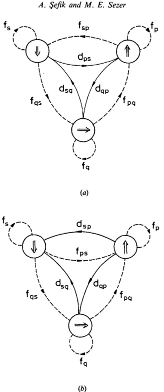
Let us denote, for convenience, the pair of edges f.. and d,

associated with each pair (f;,jj), i,j = p, q, s, i # j, by fu and du. Then, condition ( ii)' implies that !0( 5') contains a subgraph which is isomorphic to one of the basic structures shown in Fig. I. (There are eight possible combinations of different orientations of the edges fu, i,j = p, q, s, i # j, but six of these are essentially the same as one of the other two except for a relabelling of p, q and s.)

However, each of these subgraphs contradicts condition (i), the one in Fig. l(a)

containing a cycle which includes three /-edges, J;,., /sp and f .... and the one in Fig.

I (b) containing a cycle which includes two /-edges J;,. and f.s· Therefore, !0( 5')

cannot contain three disjoint /-cycles. It cannot contain four or more pairwise disjoint /-cycles either, because this necessarily includes the existence of three pairwise disjoint /-cycles. This completes the proof of Fact I. D

Fact 2

The correspondence between the (f.., d,)'s statement of condition (ii)' is one-to-one.

Proof of Fact 2

and the pairs of (f,.,f.)'s in the

D

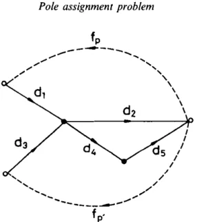
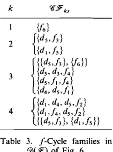
If (/.., d,) corresponds to two distinct pairs (J;,,f.) and (/,.·./.-) then either all cycles formed by J;, and J;,· or all cycles formed by f. and f.· should cover the same state vertices. Suppose, without loss of generality, that the former is true and that p < p'. Since fp· appears in '115';., which is of width p', then so does

JP in some 'll!f'P. of width p'. However, every d-edge in ((f!f'P. appears either in

'115';. or in '115';, which violates condition (iii)( b). The situation is illustrated in Fig. 2, where p =I, p' = 2, '115'; = {d_1, d2

,J;,},

Cfl:F; = {d3, d4, d5,f,.·} and

'll!f'P.

=

{d_1, d_4, d₅,f,. }. D

Fact 3

Suppose the pair (/, d,) corresponds to the (unique) pair (J;,,f.). If/, appears in a product term in some gk(f) of (12), then so does the productfJ., and vice versa. Moreover, all the product terms that contain f.. in any gk( f) are of the form eh(e,f..

+

eP.J;,f.), where ek, e, and epq are polynomials in d with e, and epq

being the same in all such expressions. D

Proof of Fact 3

Let Cfl,., _{'lle2, ... ,} denote all simple /-cycles formed by f..; and for each i, let

'llff di" Cflffdi2, ... , denote all d-cycle families which have no vertex in common with

'll,i· Then, any simplef-cycle family containing/.. is of the form 'llff,

=

'11, u'lldij for some i and j, so that w('IJS',) = w('ll,;) x w('lldi)

=

e,if..edij· By condition (ii)', to every Cfl, there correspond disjoint simple /-cycles 'llpi and 'llqi formed by JP and f.,

which are also disjoint from all 'lldij· Therefore, they form an /-cycle family

'llffpq

=

'llpi u '11qi u 'lldij of the same width as that of '115', and having the weight

w('llff pq) = ePJP x e.J. x edij· This shows the existence of the product JJ.

wherever f.. appears. The converse is also true, and the proof of the first part is Proof of Fact 1

Suppose that 9097) contains three pairwise disjoint f—cycles formed by the

f-edges f,,, f,, and L. Let us denote, for convenience, the pair of edges f, and d,

associated with each pair (fi,fj), i, j = p, q, s, 1' ¢ j, by f0- and do“ Then, condition (ii)’ implies that 9(9) contains a subgraph which is isomorphic to one of the basic structures shown in Fig. 1. (There are eight possible combinations of

different orientations of the edges fij, i,j=p,q,s, iyéj, but six of these are

essentially the same as one of the other two except for a relabelling of p, q and 3.) However, each of these subgraphs contradicts condition (i), the one in Fig. 1(a) containing a cycle which includes three f-edges, q, f,” and few and the one in Fig. |(b) containing a cycle which includes two f—edges q and f,,,. Therefore, 9L9?) cannot contain three disjoint f-cycles. It cannot contain four or more pairwise

disjoint f—cycles either, because this necessarily includes the existence of three

pairwise disjoint f-cycles. This completes the proof of Fact 1. El

Fact 2

The correspondence between the (f,,d,)’s and the pairs of (f,,,fq)’s in the

statement of condition (ii)’ is one-to-one. El

Proof of Fact 2

If (f,,d,) corresponds to two distinct pairs (finfq) and (f‘,,.,fq.) then either all cycles formed by ft? and f, or all cycles formed by fq and fq> should cover the same state vertices. Suppose, without loss of generality, that the former is true and that p <p’. Since fp appears in (fife-3", which is of width p’, then so does j; in some (637,, of width 17'. However, every d-edge in (697,, appears either in (6347; or in (63523 which violates condition (iii)(b). The situation is illustrated in

Fig. 2, where p = l, p' =2, (6.97: = {d., d2,fp}, @975: {(13, d4,d5,j;,.} and

(69—F.={d,,d4,d5,fp}. D

Fact 3

Suppose the pair (f,, d,) corresponds to the (unique) pair (finfq). Iff, appears in a product term in some gk( f) of (12), then so does the product fflfq, and vice versa. Moreover, all the product terms that contain f, in any gk( f) are of the form ek,(e,f, + epqfifq), where eh, e,, and em are polynomials in d with e, and em

being the same in all such expressions. D

Proof of Fact 3

Let %’,.,‘€e2, ..., denote all simple f-cycles formed by f,; and for each i, let (65%”, (gym, ..., denote all d-cycle families which have no vertex in common with g". Then, any simplef-cycle family containingf, is of the form @317, = (6,, u‘gdij for some i and j, so that 006637,) =w(‘6,,.) x (906%.) = e,,-f,e,,,j. By condition (ii)’, to every (6,,- there correspond disjoint simple f-cycles ‘6’,” and fl, formed by f,, and fq, which are also disjoint from all (61,0. Therefore, they form an f-cycle family (6.977” = (gp,vu%q,v‘6m of the same width as that of (6797,, and having the weight (Baggy!) = emfp x eq,fq x edij. This shows the existence of the product fnfq

982

A. Sefik and M. E. Sezer

\

\ I I

'

fqs \ I I \ I I fqs ' \

'

'

_'

_'

'

'

_',,

(a) (b) ... - .... fp I \ I I I dqp I I / fpq / / / I I I dqp / / / /

l

fpq I I /

Figure I. The two basic structures mentioned in the proof of Fact I.

complete. Now, let e, be the product of the weights of the d-edges which are

common to all C,;, but do not occur in some <(JP, u<(J.,. Obviously, d, appears in e,

so that e,,

=

e;, x eP. Also define eP and e. to be the products of the weights of the d-edges which are common to all <(JP, and <(!•'' respectively, and which do not appear

in some C,;, and therefore write eP, = e~, x eP and e., = e~, x e •. Since for fixed i,

rtP,

uC(/•' and rJ,, cover exactly the same state vertices, then eP and e. may

982 A. Sefik and M. E. Sezer

(b)

Figure l. The two basic structures mentioned in the proof of Fact I.

complete. Now, let e, be the product of the weights of the d—edges which are common to all C,,., but do not occur in some 49”,,- u‘gqi. Obviously, d, appears in e,,

so that e,,- = e; x ep. Also define e, and e, to be the products of the weights of the

d-edges which are common to all g,”- and (éqi, respectively, and which do not appear in some C,,, and therefore write epi = egfi x e” and eqi = e;,» x e,,. Since for fixed i, ’6’,"- u‘gq, and %,,~ cover exactly the same state vertices, then 2,, and eq may

Figure 2. Illustration of the situation mentioned in the proof of Fact 2.

only contain weights of d-edges that are adjacent either from the input or to the output associated with J;, and f., respectively. Furthermore, e;,

=

e~, x e~,. Then,

w('t?ff,)

+

w('t?ffpq)

=

e;,ed1j(e,f,

+

ePe.J;,f.) independent of the widths of the cycle

families 'tfff, and 't?ffpq• and the proof follows. 0 Now, returning to the proof of Theorem 2, Fact together with condition (i) imply that each product term w('t?ff) in ( 12) contains at most two variable weights. Also, defining

0

=

{k \fk forms a cycle which is disjoint from some other /-cycle}

and

f..

as in ( 13) with

e,

= e, and

1/1,

= eP.fPf., Fact 3 guarantees the structure in ( 12). The rest of the proof is the same as that of Theorem I. 0

The usefulness of Theorems I and 2 depends largely on the choice of the n feedback gains to the included in/, as well as on the choice of the zero or non-zero fixed values to be assigned to the remaining feedback gains in

fc.

An algorithm, which determines whether such a choice of n feedback edges that satisfy the conditions of Theorem 2 exists, is given in the Appendix.

4. Examples of generically pole assignable systems

In this section we show that certain classes of systems which are known to be generically pole assignable by state or dynamic output feedback satisfy the condi-tions of Theorem 2 and thus demonstrate that Theorem 2 characterizes a non-trivial class of pole assignable structures.

4.1. Structurally controllable systems with state feedback

Consider a system described by

f/: x=Ax+Bu ( 16)

Figure 2. Illustration of the situation mentioned in the proof of Fact 2.

only contain weights of d-edges that are adjacent either from the input or to the

output associated with fp and fa, respectively. Furthermore, e',,- =4". x egfl. Then,

006637,) + w(‘697pq) = e’,,.ed,.j(e,fi + epeqfq) independent of the widths of the cycle

families (63’4", and ‘69”, and the proof follows. U

Now, returning to the proof of Theorem 2, Fact 1 together with condition (i) imply that each product term (0663‘) in (12) contains at most two variable weights. Also, defining

l] = {k lfk forms a cycle which is disjoint from some other f-cycle}

and f, as in (13) with 6‘, = e, and w, = eqpfq Fact 3 guarantees the structure in (12). The rest of the proof is the same as that of Theorem I. C] The usefulness of Theorems 1 and 2 depends largely on the choice of the n feedback gains to the included in L, as well as on the choice of the zero or non-zero

fixed values to be assigned to the remaining feedback gains in fl. An algorithm,

which determines whether such a choice of n feedback edges that satisfy the conditions of Theorem 2 exists, is given in the Appendix.

4. Examples of generically pole assignable systems

In this section we show that certain classes of systems which are known to be generically pole assignable by state or dynamic output feedback satisfy the condi-tions of Theorem 2 and thus demonstrate that Theorem 2 characterizes a non-trivial

class of pole assignable structures.

4.1. Structurally controllable systems with state feedback

Consider a system described by

984 A. $efik and M. E. Sezer

and the full state feedback law

:F: u = Fx ( 17)

where x e IR" and u e !Rm. Since .'F is a special case of static output feedback with states considered as outputs, the resulting closed-loop system Sf'( :F) can be represented by the reduced system structure matrix

S(F) =

[~

:]

(18)

Let the corresponding open- and closed-loop system digraphs be

~,.,.=(ffuo//,r!,.J and ~,_A:F)=(fifuo//,r!,xur!F)· We now state our main result concerning Sf'( :F).

Theorem 3

The following are equivalent: (a) 5f' is structurally controllable;

(h) Sf'( :F) is generically pole-assignable;

(c) there exists a choice of n feedback edges such that when the remammg feedback edges are assigned suitable fixed weights, ~,_A.'F) satisfies the

conditions of Theorem I. 0

The proof of Theorem 3 is based on the following two lemmas.

Lemma 3

Let ~c

=

(f!f u {u }, r!) be a cactus. Then there exists an enumeration of the state vertices such thaI

(a) if x1 is on a non-terminal bunch and xj is on the terminal bunch, then i <j; (h) if (x,, x) e r! and xj is not the tail of the distinguished edge of some bud, then j

=

i

+

k

+

I, where k is the total number of state vertices on the

precactus with origin x,. 0

Proof

Using a modified depth-first search algorithm (Tarjan 1972), scan first the non-terminal bunches (if there are any) in any order, and last the terminal bunch of ~c, and assign the integers I, 2, ... , n to the state vertices during the scanning process according to the following simple recursive scheme. Let the current vertex being visited be x,. If there is a cactus or precactus with origin at

x,,

then replace

~c by this cactus or precactus (with x, taking the role of u) and repeat. Otherwise, let the unique vertex adjacent from x, be x*. If x* is not yet assigned an integer, let i +-i

+

I, x,

=

x *, and repeat. Otherwise, x

*

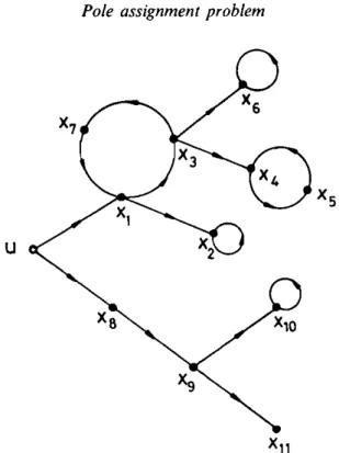
should be adjacent from the root of the cactus currently being scanned. Continue with another bunch. 0

It is obvious that this scanning of ~c results in an enumeration of the state vertices which satisfies the requirements. To illustrate the scheme, enumeration of the vertices of a simple cactus is shown in Fig. 3.

984 A. Sefik and M. E. Sezer

and the full state feedback law

? : u = Fx ([7)

where x e R” and u e R’". Since .97 is a special case of static output feedback with states considered as outputs, the resulting closed-loop system 913") can be represented by the reduced system structure matrix

A B

S(F)=[F 0]

(18)

Let the corresponding open- and closed-loop system digraphs be

9,“. : (Quail, (5,“) and 9“,.(5’) = (fitfll, 6’“. U6;). We new state our main result concerning 9(9).

Theorem 3

The following are equivalent:

(a) .9’ is structurally controllable;

(1)) 9(9) is generically pole-assignable;

(c) there exists a choice of n feedback edges such that when the remaining feedback edges are assigned suitable fixed weights, 9,”.(37) satisfies the

conditions of Theorem I. E]

The proof of Theorem 3 is based on the following two lemmas.

Lemma 3

Let 9;. = (9f u {u}, at") be a cactus. Then there exists an enumeration of the state vertices such that

(a) if x,- is on a non-terminal bunch and x}. is on the terminal bunch, then 1' <j; (b) if (xi, xj) e (6’ and xj is not the tail of the distinguished edge of some bud, then j =1” +k + I, where k is the total number of state vertices on the

precactus with origin xi. C]

Proof

Using a modified depth~first search algorithm (Tarjan 1972), scan first the non-terminal bunches (if there are any) in any order, and last the terminal bunch

of 9c, and assign the integers 1,2, ..., n to the state vertices during the scanning

process according to the following simple recursive scheme. Let the current vertex

being visited be xi. if there is a cactus or precactus with origin at x,, then replace 9c by this cactus or precactus (with x, taking the role of u) and repeat. Otherwise, let the unique vertex adjacent from x,- be x“. If x* is not yet assigned an integer, let it—i’ -+- l, .t',- = x“, and repeat. Otherwise, x“ should be adjacent from the root of the cactus currently being scanned. Continue with another bunch. C]

It is obvious that this scanning of 9C results in an enumeration of the state vertices which satisfies the requirements. To illustrate the scheme, enumeration of the vertices of a simple cactus is shown in Fig. 3.

u

x,,

Figure 3. Enumeration of the state vertices in a cactus.

Lemma 4

Let S =(A, B) be structurally controllable. Then there exists a fixed feedback

matrix F1 and a column b, of B such that

(a) the non-zero elements of A+ BF, and b, are algebraically independent, and

(b) the system S, =(A+ BF1 , b,) is structurally controllable. 0

Proof

If (A, b;) is structurally controllable for some i, let F1

=

0. Otherwise, let !0ux be

spanned by a union of cacti !0c,, !0c2 , ••• , !0ck with roots

u,,,

u,₂, •.• ,

u,,

and tips

Xn_1, Xn₁ +n₂, ... , Xn₁ + ... +n.~r' where l ~ k ,:::; m, 1 ~ i, < ... < ik ~ m, and n₁

+

n2

+ ... +

nk

=

n. Let F1

= (

J;,.)

with

f,

={1,

ifp=i1,q=n1+ ... +n1_.,forsome2~/~k

pq 0, otherwise

and let i

=

i1 • Then, since the elements of (A, B) are algebraically independent and

non-zero elements of F1 are fixed as unity, the elements of (A+ BF,, b,) are also

algebraically independent. Moreover, S, is spanned by a cactus obtained by making the roots of !0c.l+ 1 coincide with xn, + ... +n,, I= I, ... , k- I. 0

Note that Lemma 4 is a structural counterpart of the well-known algebraic result (Davison and Wang 1973) that if (A, B) is controllable, then for almost all

F_{1 ,} (A

+

BF,, b,) are controllable.

Figure 3. Enumeration of the state vertices in a cactus.

Lemma 4

Let S = (A, B) be structurally controllable. Then there exists a fixed feedback matrix F, and a column b,- of 8 such that

(a) the non-zero elements of A + BF, and b,- are algebraically independent, and (b) the system S1 = (A + BF. , bi) is structurally controllable. Cl

Proof

If (A, b,) is structurally controllable for some i, let Fl = 0. Otherwise, let 9,“ be spanned by a union of cacti fichgcz, ...,9ck with roots uil,u,-2, ..., Nil: and tips X111: x,,I+,,2, ...,x,,1+m+,,k, where l <k gm, l S i1 < <ik gm, and HI +n2+ ...+ In =n. Let F, =(q) with

f _ I, ifp=i,,q=n.+...+n,_,,forsomeZSl'sk

”q_ 0, otherwise

and let i = i.. Then, since the elements of (A, B) are algebraically independent and non-zero elements of F. are fixed as unity, the elements of (A + BF., bi) are also algebraically independent. Moreover, Sl is spanned by a cactus obtained by making the roots of 92a,“ coincide with xnl+m+,,,, I: 1, ...,k — l. I] Note that Lemma 4 is a structural counterpart of the well-known algebraic result (Davison and Wang 1973) that if (A, B) is controllable, then for almost all Fl , (A + BF. , b,-) are controllable.

986 A. Sefik and M. E. Sezer

We now prove Theorem 3.

Proof of Theorem 3

Owing to Lemma 4, is suffices to give the proof for the single-input case. (a)~ (b): Obvious.

(c) =>(b): Theorem I.

(a)=> (c): Let the system digraph !i&ux be spanned by a cactus !1&0, whose state

vertices are enumerated as in Lemma 3. Let the feedback edges be enumerated in the same way so that/; = (x,, u), i = I, 2, ... , n. Since all /-cycles in !!&.A$') pass through vertex u, conditions (i) and (ii) of Theorem I are readily satisfied. The

enumeration of the state vertices guarantees that for i = I, 2, ... , n, any state vertex

xj with j ~ i either lies on the complementary path of/; in !i&c( .9'), and hence

belongs to thef-cycle defined by/;, or belongs toad-cycle in !1&0(.9') which has no

vertex in common with the complementary path of/;. Let <(1.9'1 denote the union of these cycles in!!&( .9'). Obviously, <(Jff1 is a simplef-cycle family of width i which contains /;. (For example, referring to Fig. 3, <(Jff6 consists of the f-cycle {(u, x, ), (x1 , x3 ), (x3 , x6 }, (x6 , u)} and the d-cycles {(x2 , x2 )} and {(x4 , x5 ), (x5 , x4 }.)

This proves condition (iii)(a) of Theorem I. Now, let <(Iff, be any simple /-cycle family of width i which includes an /-edge jj for some j < i. If <(Iff, contains a d-edge which does not belong to the edge set of !1&0 , then this edge does not appear

in any <(Jfff, and condition (iii)(b) of Theorem I is readily satisfied for <(Iff,.

Suppose all the d-edges of <(Iff, belong to !1&0• Since <(Iff, covers exactly i vertices, it covers a vertex xk with k ;;. i. Then, the edge originating from xk in <(Iff, is a d-edge (the only f-edge in <(Iff, is jj which originates from

xJ

which does not appear in any <(Jfff, I~ k. Again, (iii)( b) is satisfied. This completes the

proof. 0

4.2. A class of structurally controllable and observable systems with dynamic output feedback

Consider a single-input/single-output system //': x=Ax+bu}

y

=

CTX

to be con trolled by a dynamic output feedback of the form

(19)

(20)

where

.i

e lkl'1 _{is the state of the controller}

_.<?.

_{It is well known (Davison and}

Chatterjee 1971) that the closed-loop system consisting of Y' and

.<?

is the same as the one obtained by applying a constant output feedback of the form

(21)

986 A. Sefik and M. E. Sezer

We now prove Theorem 3. Proof of Theorem 3

Owing to Lemma 4, is suffices to give the proof for the single-input case. (a) ¢> (b): Obvious.

(c) => (b): Theorem I.

(a) => (c): Let the system digraph 9“ be spanned by a cactus 90, whose state vertices are enumerated as in Lemma 3. Let the feedback edges be enumerated in the same way so thatf, = (x,, u), 1': l, 2, ...,n. Since all f—cycles in 9“,,(9’) pass through vertex u, conditions (i) and (ii) of Theorem I are readily satisfied. The

enumeration of the state vertices guarantees that for i = l, 2, ..., n, any state vertex

xj with j st either lies on the complementary path off,- in @437), and hence belongs to thef-cycle defined by f,, or belongs to a d-cycle in 949') which has no vertex in common with the complementary path of 12-. Let (69’3“ denote the union of these cycles in 90?). Obviously, (697:? is a simple f—cycle family of width 1‘ which contains f,. (For example, referring to Fig. 3, (6.97: consists of the f-cycle

{(u, x.), (x. , x3), (x3, x6), (x5, u)} and the d-cycles {(x2, x2)} and {(x4, x5), (x5, x4}.)

This proves condition (iii)(a) of Theorem I. Now, let (697, be any simple f—cycle family of width i which includes an f-edge f}. for some j <i'. If (6’33, contains a d-edge which does not belong to the edge set of 9c, then this edge does not appear in any ‘69:}, and condition (iii)(b) of Theorem I is readily satisfied for (63",. Suppose all the d-edges of (6’97, belong to 9%. Since (6?, covers exactly 1‘ vertices, it covers a vertex xk with k >12 Then, the edge originating from xk in (6.97,» is a d-edge (the only f-edge in (673/7, is fj which originates from x) which does not appear in any (697, [<k. Again, (iii)(b) is satisfied. This completes the

proof. Cl

4.2. A class of structurally controllable and observable systems with dynamic

output feedback

Consider a single-input/single-output system

5”: x=fix+bu} (19)

y = c x

to be controlled by a dynamic output feedback of the form

57’ ‘ = x? ‘ b“

X .T. + y

(20)

u = c x +fy

where f E R“ is the state of the controller 57’. It is well known (Davison and Chatterjee 197]) that the closed-loop system consisting of 5” and 9 is the same as the one obtained by applying a constant output feedback of the form