Modelling the public sector deficit and inflation relationship in Turkey

9 Л5І ^r ^ g_- - ^ -. -T . : V ^ ^ -4c

■

„іч^ь ■

и u ГЕ OF

4KOAJ -ÜLFILı„iVIENT

REQUÎREMEMTS

MODELLING THE PUBLIC SECTOR

DEFICIT AND INFLATION RELATIONSHIP

IN TURKEY

A THESIS PR E SE N T E D B Y H A N A JALEL TO

TH E IN S T IT U T E OF

E C O N O M IC S A N D SO CIAL SCIENCES IN PAR TIAL FU LFILLM E N T OF TH E

R E Q U IR E M E N T S

FO R TH E D EG R E E OF M A S T E R OF E C O N O M IC S

B IL K E N T U N IV E R S IT Y A U G U S T , 1997

Н(а

I certify that I have read this thesis and in my opinion it is fully adequate, in scope and in quality, as a thesis for the degree of Master of Economics.

Assist. Prof. Kıvılcım Metin

I certify that I have read this thesis and in my opinion it is fully adequate, in scope and in quality, as a thesis for the degree of Master of Economics.

1 certify that I have read this thesis and in my opinion it is fully adequate, in scope and in quality, as a thesis for the degree of Master of Economics.

ssist. Prof. Izak Atiyas Approved by the Institute of Social and Economic Sciences

A C K N O W L E D G E M E N T S

I am grateful to Assist.Prof. Kıvılcım Metin for her supervision and guidance throughout the development of this thesis. I would like also to express my grat­ itude to Aylin Ozey from Turkish Treasury and Özlem Başçı for their help and guiding comments.

My foremost thanks go to my family and especially to my father for their endless support and encouragements throughout all my years of study. And last gratitude is to my dearest Serdar for his moral support in my hardest days. Finally, I would like to dedicate this thesis to my father.

A B S T R A C T

MODELLING THE PUBLIC SECTOR DEFICIT AND INFLATION RELATIONSHIP

IN TURKEY HANA JALEL

MASTER OF ECONOMICS Supervisor; Assist.Prof. Kıvılcım Metin

August, 1997

This study assesses the empirical relationship between the public sector deficit and inflation in Turkey using the cointegration analysis. Since 1986, the Treasury set a consistent, well defined institutional framework to monitor the selling of government bonds and bills in order to finance budget deficit of Turkey besides the issuance of base money by the Central Bank. Inflation is estimated by using scaled budget deficit, growth rate of real income, scaled stock of bonds, scaled interest paid and scaled base money. First, the time series properties of the data set are examined then, weak exogeneity of the independent variables and cointegration are tested. Next, both a single equation and a VAR model are estimated. Weak exogeneity and cointegration tests show that a VAR model is more reliable than a single equation model. The estimation of a VAR model indicates that inflation in Turkey is related solely to its first lag, implying that the Turkish inflation is inertial with about 35% of inertia.

Key Words: Turkish Inflation, Government Bonds, Base Money, Cointegration, Weak Exogeneity, VAR model.

oz

TÜRKİYE’ DE KAMU SEKTÖRÜ AÇIĞI İLE ENFLASYON ARASINDAKİ İLİŞKİNİN

MODELLENMESİ HANA JALEL

Yüksek Lisans Tezi, iktisat Bölümü Tez Yöneticisi: Yrd.Doç.Dr. Kıvılcım Metin

Ağustos, 1997

Bu çalışma, Türkiyede kamu sektörü açıklan ile enflasyon arasındaki ampirik ilişkiyi, eş-bütünleşme yöntemini kullanarak açıklamaya çalışmaktadır. 1986 yılından beri. Hazine Genel Müdürlüğü, hazine bonosu ve tahvil ihraç ederek kamu sektörü açığını finanse etmektedir. Dolayısıyla, Merkez Bankasının para basarak bütçe açığını finanse etmesi olgusu göreli olarak azalmıştır. Tezde enflasyon, bütçe açığı, reel gelirin büyüme hızı, bono stoku, faiz ödemeleri ve baz para tarafından açıklamaya çalışmıştır. Bu tezde öncelikle veri setinin zaman serisi özellikleri incelenmiş, daha sonra zayıf dışsallık ve eş-bütünleşme test edilmiştir. Daha sonraki aşamada, hem bir tek denklemli model ve hemde kapalı sistem VAR modeli tahmin edilmiştir. Zayıf dışsallık ve eş-bütünleşme testleri, VAR modelinin tek denklem tahmininden daha güvenilir olduğunu belirlemiştir. VAR modelinin tahmini enflasyonun, yanlızca bir dönem önceki geçmiş değeri ile açıklanabildiğıni göstermiştir, ve dolayısıyla Türkiyedeki enflasyonun yaklaşık %35’inin inertial bir enflasyondan kaynaklandığı, ve enflasyon olgusunun kendisi beslediği ortaya konulmuştur.

Anahtar Kelimeler: Türkiyede Enflasyon, Hazine Bonoları, Baz Para, Eş-bütünleşme, Zayıf Dışsallık, VAR Modeli.

Contents

5.2 Results of Unit Root Tests ... 24

5.3 Results of Cointegration Test 26 5.4 Results of Weak Exogeneity Test 28 6 E M P IR IC A L M O D ELLIN G 30 6.1 Single Equation A n a lysis...30

6.2 VAR M o d e l ...34

7 C O N C LU SIO N 39

• Table 1. The Data Set

• Table 2. Results of Unit Root Tests for the First Data Set

Table 2.1. ADF Tests for 1(0) Table 2.2. ADF Tests for 1(1) Table 2.3. ADF Tests for 1(2)

• Table 3. Results of Unit Root Tests for the Second Data Set

Table 3.1. ADF Tests for 1(0) Table 3.2. ADF Tests for 1(1)

• Table 4. Schwarz and Hannan-Quinn Information Criteria on the Length of Lags

• Table 5. Johansen Tests for the Number of Cointegrating Vectors

• Table 6. Results of Exogeneity Tests

• Table 7. Correlation Matrix

• Table 8. Single Equation Estimation Results

• Table 9. Single Equation Estimation Results Including k

• Table 10. Single Equation Estimation Results Including k, h*, b*

APPENDIX A

APPENDIX B

Graph 1. Graphs of Base Money Graph 2. Graphs of Budget Deficit

Graph 3. Graphs of Consumer Price Index Graph 4. Graphs of Stock of Bonds

Graph 5. Graphs of Interest Paid Graph 6. Graphs of Real GNP

Graph 7. Graphs of Scaled Budget Deficit Graph 8. Graphs of Scaled Interest Paid Graph 9. Graphs of Scaled Base Money Graph 10. Graphs of Scaled Stock of Bonds Graph 11. Graphs of D and h*

Graph 12. Graphs of D and 6* Graph 13. Graphs of R and b* Graph 14. Graphs of D and Inflation Graph 15. Graphs of g and Inflation Graph 16. Graphs of g ajid D

1

INTRODUCTION

High inflation rates have been a major item on the agenda of the Turkish economy since 1977. And despite all the intentions to bring down the inflation in Turkey, it still remains as a major economic problem of the economy. For the last two decades, agents in the economy have experienced an accelerating inflationary process that de- stroyed both the economic and social balances while blurring the relation between al)solute and relative prices (Koray, 1993).

Although an extensive literature tried to consider the reasons behind this accel­ erating inflationary process, and to examine its relation with other flscal macroeco­ nomic variables such as the public sector deficit, high inflation rates are still on the agenda of the Turkish Economy.

Many studies such as Dornbush and Fischer(1981), Buiter and Patel(1992), Metin (1995), King and Plosser(1985) that investigated the relationship between the growth rate of deficit and inflation for both developed and developing countries did not give concrete results that supports the relationship between budget deficit and inflation both in the short run and in the long run.

For Turkey, Ozatay(1996) emphasizes the importance of coordination of fiscal and monetary policies in achieving price stability. But he shows that the persistent budget deficits of the Turkish economy make this property not sufficient to achieve price stability.

Metin(1995) found that fiscal expansion was an explanatory variable for infla­ tion. Also, the study yielded a positive significant relation between excess demand

for money and inflation in the short run but a small effect from imported inflation and excess demand for assets in the capital markets. Finally, the study yielded no significant relation between inflation and excess demand for goods. The result of the study was that elimination of budget deficits could rapidly reduce inflation.

Metin(1996), using the public finance approach to inflation for the period 1950- 1988 found that financing budget deficits by printing money solely, has been the main reason for inflation in Turkey. She analyzed this causality by using the re­ cent econometric methods such as unit root tests and cointegration tests as well as disequilibrium analysis. Theoretically, Sargent and VVallace(1981) have found a close result. They have shown in their seminal article that if the time paths of G and T are fixed, under some conditions, bond-financed deficits are non-sustainable so monetization of the deficit will carry on. This results in an increase in money supply and therefore in a rise in the rate of inflation in the long run.

The major concern of this work is that the public sector deficit is financed by issuing money and government bonds and bills starting from the late 1986’s. The theoretical framework is based on an assumption of closed economy which is a re­ strictive assumption for the Turkish economy, so the results found in this work may also be very restrictive. Moreover, it should be noted that the results of this work may be very different from the results that can be obtained under an open economy assumption. The assumption of a closed economy can be relaxed in a future work by including the exchange rate or net export earnings in the economic framework.

theory. It is based on the multivariate cointegration theory developed by Johansen (1988), on the weak exogeneity concepts and on the modelling framework suggested by Johansen and Juselius(1990) and Hendry and Mizon(1993).

T1 le work consists of modelling the relationship between the public sector deficit and inflation using the following macroeconomic variables: scaled budget deficit, scaled base money, scaled stock of bonds, scaled interest paid and growth rate of I’cal income.

Accordingly, the rest of the study is organized as follows. In chapter 2, the historical background of the Turkish economy since 1980 is discussed. In chapter 3, the econometric theory used in this study is explained. In chapter 4, a theoretical framework depending on the public finance approach is developed. In chapter 5, the data set is described and the results of the unit root tests, weak exogeneity tests and cointegration tests are examined. In chapter 6, both an autoregressive distributed lag model (ADL) and a vector autoregressive model (VAR) are developed and estimated. Finally, in chapter 7, the concluding remarks that can be drawn from the empirical results are discussed. The related tables and graphs are reported in Appendix A and Appendix B respectively.

2

HISTORICAL BACKGROUND

In 1980, and as a result of the 1970’s problems (increase in world price of oil, transfer ])a,yments to SEEs, large salary increases for civil servants, ect ...), inflation reached 100%. It was fed by monetization of public sector deficits. The 1980 stabilization program aimed to reduce inflation by creating more efficiency in the operation of SEEs, limiting growth of government expenditure, reducing subsidies and attempt­ ing to improve revenue collection.

The reforms implemented after 1980 were firstly successful, for they decreased infla­ tion from 100% to 35% in 1982. But after 1982. inflation rose again and remained as a problem throughout the 1980s.

In January 1990, the Central Bank publicly announced its first monetary pro­ gram which aimed at controlling inflation. The Central Bank did not announce a monetary program for 1991 mainly because of the Gulf war as well as increasing l)udget deficits. In 1992, the Central Bank reluctantly made the second program public eventhough there were no substantial corrective measures on the fiscal side. This program was not as successful as the one announced in 1990, because it failed to adhere to its targets.

In 1993, The Central Bank avoided announcing a monetary program because of increasing budget deficits. And in 1994, a very severe financial crisis emerged. In order to manage the crisis, the government negotiated with the IMF which put tight limits on the Central Bank’s balance sheet.

ing a price stability goal (Ozatay 1996), the Turkish experience, as is discussed above, shows that this is not sufficient to reach price stability in countries with persistent budget deficits.

The chronic and high rate of budget deficits in Turkey are of great concern because 1 hey are believed to have raised problems about the sustainability of the current fis­ cal situation, especially inflation.

Also, the main instruments which the Turkish Treasury uses in financing the gov­ ernment budget deficit are of great importance because they are believed to affect the sustainability of the fiscal situation given that high rates of budget deficits stem mainly from the interest payments of government debts.

When the development of Turkey’s domestic borrowing is examined, it can be noticed that from the beginnings of Republic to the sub 1970’s, governments had re­ sorted to borrowing rarely and government papers could be issued only in accordance with special borrowing laws.Financing the government deficit through the issuance of l3onds and bills is relatively a new phenomenon in Turkey. Although, the budget deficit is a persistent matter of concern in Turkey for years, domestic borrowing via issuance of bonds and bills has not always been the continuous measure to which the governments resorted in the past. The usual way of closing the gap between the government revenues and outlays have been to use the Central Bank advances and sliort term borrowing from the Central bank as well. But, both the size and the composition of domestic Tresury borrowing have changed significantly since 1980.

rowing policies. By the end of 1980, debt consolidations accounted for 47% of the total debt. By the end of 1988 the ratio had risen to 67% under the impact of large Central Bank foreign exchange losses assumed by the Treasury. The share of this kind of Treasury obligation was then reduced down to 51% in 1990 as a result of l:)oth relatively slow depreciation of TL against other currencies and repayments of some consolidated debt to the Central Bank. The share of Central Bank Advances was 27% in 1980. It fell down to 5 % in 1990 as the Treasury shifted from moneti­ zation of the debt to issuing of bonds and bills. As a result of this shift, the share of bonds and bills rose from 26% in 1980 to 44% in 1990. After 1990, the share of Central Bank advances in financing the Turkish budget deficit continued to de­ cline sharply reaching a value of 3% in 1996. The increased resorting to issuance of l)onds and bills has been accompanied by a gradual shift toward longer maturities, in an effort to reduce annual gross borrowing requirements as well as interest payments.

Treasury financing through the issuance of government paper in the domestic pri­ mary market have some interesting features which developed in the last ten years. Although Treasury had attempted to sell bonds and bills to the public, especially to finance the military engagement in Cyprus in 1974, it was not before May 1985 that the Treasury set a consistent, well defined institutional framework to monitor t he selling of government bonds and bills through auctioning.

Presently, there are two main government papers sold on auction basis, govern­ ment bonds and treasury bills. The government bonds are instruments with one \*ear or longer maturities. Treasury bills have maturities with less than one year. In cither words, the main difference between these two instruments comes from their

All the treasury bills and one year government bonds are zero coupon securi­ ties and sold discounted through auctioning. As the fiscal agent of the Treasury, the Central Bank handles the auction procedure and on Friday of every week, the amount to be sold is announced by the Central Bank through sending fax messages to the banks and other financial institutions. The anjiouncement also appears on Reuter Screens.

maturities.

In October 1988, Treasury introduced a new scheme called ’’ Tapping” , with a view to lengthen the maturity of domestic borrowing and to seek a relief in interest payments. Treasury places variable interst rate bonds with the central bank to be sold to the investors on their request. The bonds remain the property of the Trea­ sury until the investors decide to tap these bonds from the Central Bank. The latter serves as an intermediary, or a depository and neither buys nor sells these bonds during the tapping procedure. Interest is paid quarterly, semi-annually or annually and the maturities of the bonds may vary from 2 years to 5 years or more.

In this chapter, the econometric theory used in the thesis is discused. Definitions and representations of the main tests and concepts are discussed based on a summary (Vom the book New Directions in Econometric Practice by W.W.Charemza and D.F.Deadman.

3,1

Stationarity

Stationarity of a stochastic process, in a strict sense, means that both its joint and

conditional probability distributions remain constant when time horizon is changed. Let Z{ t ) , t G T be an arbitrary stochastic process with a distribution function

F(Z{t))·, 0 () depending on t and Gj, where 0^ is a function of t also.

Z{l ),t G T is said to be stationary in a strict sense if for any subset { t i N2· •••Nn) of

T and any r,

F { Z { h ) , ..., Z { Q ) = F( Z{ U + r ) . .... + r))

that is,the distribution function of Z{ t ) , t G T is unchanged when displaced in time by an arbitrary value r.

Also any marginal distribution F{ Z { t ) ) N € T is stationarity if

F { Z{ t ) ) = F ( Z { t + T)),

and hence F( Z ( t : ) ) = F( Z( t i ) ) = ... = F( Z ( U) )

3

EC O N O M E TR IC TH EORY

111 this chapter, the econometric theory used in the thesis is discused. Definitions and representations of the main tests and concepts are discussed based on a summary from the book New Directions in Econometric Practice by W.W.Charemza and D.F.Deadman.

3.1

Stationarity

Siationarity of a stochastic process, in a strict sense, means that both its joint and

conditional probability distributions remain constant when time horizon is changed. Let Z{ t ) N G T be an arbitrary stochastic process with a distribution function

F{ Z{ t) ) ; Qt) depending on t and ©¿, where 0^ is a function of t also.

Z[ l ) , t G T is said to be stationary \n a strict sense if for any subset (^i, ¿2, ···, ¿n) of T and any r,

F{Z{ti)^ Z{tn)) = F[Z{t\ + r ),..., + t))

that is,the distribution function of Z{t)^t G T is unchanged when displaced in time

hy an arbitrary value r.

Also any marginal distribution F ( Z ( i ) ) ,i G T is stationarity if

F(Z(i)) = f (Z (( + T)),

and hence F { Z{ t i ) ) = F { Z { t 2)) — ... = F{Z{tn))

3

E C O N O M E TR IC TH EORY

attention to the means, variances and covariances of the process (Spanos, 1986). Then a stochastic process Zt is said to be stationary in a weak sense if:

E{Zt) = constant = ; Var[Zt) = constant = and:

C 0 v { Z i Z i ^ 2 ^ — CF j

Therefore both the means and the variances of the stochastic process are un­ changed in time. And, the covariance between two periods is a function of the gap between the periods only, and not the time at which the covariance is considered. If one or more of the conditions above are not fulfilled, the process is nonstation-

ary. Nonstationarity of time series is a problem in econometric analysis, because

it makes the statistical properties of the regression analysis dubious. For instance, using a nonstationary series may lead to a model that shows promising diagnostic test statistics (high large confidence intervals, homoskedasticity, no autocorre­ lation,...), even in the case where there is no sense in the regression analysis (that is the variables used in the regression may, economically, have no relationship).

The autoregressive regression shown below ,

Vt = Oi +

is stationary if |/?| < 1. Where Ct denotes a series of identically, independently dis- tributed continuous random variables with zero means.

have to be made stationary before any sensible regression analysis can be performed. A convenient way of getting rid of nonstationarity in a series is by differencing the series. Sometimes, it is necessary to difference a series more than once in order to achieve stationarity. If a series must be differenced d times to be made stationary, it is said to be integrated of order d . This is denoted as yt I{d).

3.2

Unit Root Test

In order to identify the order of integration of any variable that will be used in the regression, two tests are used. The first test is the DF test which has been proposed by Dickey and Fuller (1979). For the following first order autoregressive equation:

yt = pyt-i + Ci (1)

the DF test tests the hypothesis that p = 1, so it is a unit root test. Determining whether p is equal to one or not is important since the effect of any shock is per­ manent in the unit root {p = 1) case while the shock fades away in the other case

{p < 1). This test estimates a regression equation equivalent to equation (1), and is

given below:

Ai/i — 6yt-i + tt (2) WT can re-write equation (2) as:

2/t = (1 + ^)yt-i +

which is similar to (1) with p = (1 + ^). The Dickey-Fuller test then, consists simply of testing the negativity of 6 in the ordinary least squares regression of (2) where

the null {Ho) and alternative {H\) hypotheses are: Ho :S = (}

Hi·. 6 <Q

Rejection of the null hypothesis {8 — 0) in favor of the alternative {8 < 0) implies that the process yt is integrated of order zero. The critical values tabulated in Fuller (1976) are used to evaluate the hypothesis. The natural Student t-ratios are not used because, under a unit root, they no more have the familiar Student t-distribution.

In the case the null hypothesis cannot be rejected, we conclude that yt might be integrated of order higher than zero, or might not be integrated at all. Consequently, the next step would be to test whether the order of integration is one. If ?/i ~ 7(1), then Ayt ~ 7(0) The Dickey-Fuller equation becomes:

A A yt = 8A yt-i + ct

Tlie process of differencing yt is repeated until we establish an order of integration for i/(, or until we realize that yt cannot be made stationary by differencing.

The original Dickey-Fuller test is weak because it does not take into account possible autocorrelation in the error process et- If is autocorrelated, then the ordinary least squares estimates of equation (2) are no more efficient. The solution proposed by Dickey and Fuller (1981), is to add lags of the dependent variables to the right-hand side of the regression as additional explanatory variables, in order to approximate the autocorrelation. This test is called the Augmented Dickey-Fuller test, denoted by A D F . It is considered to be the most efficient test among all the

simple tests for integration. The ADF test is now the most widely used test.

The ADF equivalent of (2) is the following :

¿=1

The practical rule for establishing the value of k (the number of lags for Ayt-i)^ is that it should be relatively small in order to save degrees of freedom, but large enough to allow for the existence of autocorrelation in tt.

DF and ADF tests are similar tests in that they have the same structure, they test the same hypothesis and they use the same critical values. The only diference between the two tests is that the ADF test includes lagged values inorder to elimi­ nate possible autocorrelation.

3.3

Cointegration Analysis

If two (or more) nonstationary variables have a long run relationship, then the de­ viations from this long run path are stationary. If this is the case, the variables of interest are said to be cointegrated.

The formal definition of cointegration of two variables, developed by Engle and Granger (1987) is as follows:

Time series Xt and yt are said to be cointegrated of order d,b where d > 6 > 0, and written as :

1- both series are integrated of order d,

2- there exists a linear combination of these variables,say aiXt + Ci2yt^ which is integrated of order d-b .

The vector [^1 , 0 ^2] is called a cointegrating vector.

A generalization of the above definition for the case of n variables is the following: If Xt denotes an n x 1 vector of series Xu^ X2t v··^ and:

a) each of them is 1(d),

b) there exists an n x 1 vector a such that x[a ~ I{d — 6), then:

x [ a ^ C I { d , b).

For empirical econometrics, the most interesting case is where the series trans­ formed with the use of the cointegrating vector become stationary, that is where

d = 6, and the cointegrating coefficients can be identified with parameters in the

long run relationship between the variables.

Multivariate Cointegration:

The approach used to test for cointegration is the maximum likelihood procedure suggested by Johansen (1988). This procedure analyzes cointegration in a general way by directly investigating cointegration in the vector autoregression, VAR, model.

Consider the unrestricted VAR model: if:

where Zt contains all n variables of the model and tt is a vector of random errors.

All the variables in Zt will be assumed to be integrated of the same order, and tliat this order of integration is either zero or one. The VAR model, ignoring the de­ terministic part (intercepts, deterministic trends, seasonals, etc.), can be represented in the form:

k-l

^ Z t = ^ TiAZt-i + HZt-k +

¿=1 where:

Ti = —I + Ai + ... + Ai ( / is a unit m atrix)

and tt are independent, n dimensional, Gaussian, stationary variables with mean zero and variance S. Since there are n variables which constitute the vector Zt, the dimension of II is n x n and its rank can be at most equal to n. If the rank of matrix n is equal to r < n, there exists a representation of II such that:

n = a/?', where a and /3 are both n x r matrices.

+ tt (4) ¿=1

Matrix (3 is called the cointegrating matrix and has the property that f3'Zt ~ ^(0), while Zt ~ ^(1)· The columns of ¡3 contain the coefficients in the r cointegrating vec­ tors. The a matrix is called the adjustments or the loadings matrix, which measures

the speed of adjustment of particular variables with respect to a disturbance in the equilibrium relation

By regressing and Zt-k on AZ^_i, AZ^_2, AZt-k-\-i we obtain residuals Rot

and Rkt^ The residual product moment matrices are, T

Sij = T~^ ^ RitR^j^^ i^j = 0, A: ( r = sam plesize) t=i

Solving for eigenvalues,

If^Skk *S/jO*Sqq 5*0A; I — 0,

yields the eigenvalues /¿i > /12 > ··· > /¿n (ordered from the largest to the smallest) and associated eigenvectors Vi which may be arranged in the matrix

V = [ui, O2 , O n ] · The eigenvectors are normalized such that V'SkkV = R If the cointegrating matrix ¡3 is of rank r < n ,the first r eigenvectors are the cointegrating vectors, that is they are the columns of matrix Using the above eigenvalues, t he null hypothesis that there are at most r cointegrating vectors can be tested by calculating the loglikelihood ratio test statistics:

LR — —T ^ / n ( l —/¿¿),

2 = r-|-l

which is called the trace statistic (Johanses and Juselius (1990)). Normally test­ ing starts from r=0 , that is from the hypothesis that there are no cointegrating \ ectors in a VAR model. If this can not be rejected the procedure stops. If it is rejected, it is possible to examine sequentially the hypothesis that r < l , r < 2, and so on. The null hypothesis that there are at most r cointegrating vectors, has an asymptotic distribution whose quantiles are tabulated by Johansen (1988) and

Another likelihood ratio test known as the maximum eigenvalue test in which the null hypothesis of r cointegrated vectors is tested against the alternative of r+1 cointegrating vectors. The corresponding test statistic is:

LR — —Tln{l — ¡Ir)^

The critical values of these tests are tabulated in Johansen and Juselius (1990) and Osterwald-Lenum (1992).

In empirical applications of the Johansen method, a major problem can be met when establishing the lag length, that is k in (4). If the empirical analysis is con­ cerned exclusively with the estimation and identification of a cointegrating vector, the usual practice is to allow for relatively long lags. Because, long lags might ap­ proximate the possible autocorrelation structure of the error terms. However, if the aim is to use the estimated cointegrating vector(s) for further analysis of the V A R model, using long lags may be inconsistent with economic sense. In our empirical analysis, we will use the Schwarz criteria to choose the optimal lag.

Testing and analyzing cointegration in a VAR model is often considered as su­ perior to other methods such as the Engle-Granger single equation method. The statistical properties of the Johansen procedure are generally better and the power of the cointegration test is higher. For this reason, in our empirical analysis, the .Johansen procedure is used.

3*4

Exogeneity Concepts

'Hiere are three exogeneity concepts which can be defined for a given set of parame­ ters of interest: the first one is weak exogeneity, the second one is strong exogeneity and the last one is superexogeneity. For our empirical analysis only the first one is used.

Let Xt, Yt and Zt be three stochastic processes such that their joint distribution can l)e factorized into a conditional distribution for Xt given Yt and Zt and the marginal distributions of and Zt as given below:

D[{Xt Yt , Zt ) ; Xi u\2t] Myt X3t ) MZt A4.)

where D[{Xt Yt^Zf); Ai^, \2t\ represents the dependent variable conditional on the variables of interest. D{Yt Xst) and D{Zt A4^) are the marginal processses of Yt and

Zi respectively. Xu^ X2t’> Xst and X4t are the parameters of interest.

The concept of weak exogeneity is related to the problem of static inference in an econometric model, that is estimation. Generally, a variable Zt can be regarded as weakly exogeneous for a set of parameters of interest z G if the marginal process for Zt contains no useful information for the estimation of A^-^, that is, an inference for Xit can be efficiently made conditionally on Zt alone and its marginal process contains no relevant information. The concept can also be formulated in reverse. That is, Zt is weakly exogeneous for the parameters of interest A^^, if knowledge of Xu is not required for inference on the marginal process of Zt.

Now we will examine the methodology of the time series model that will be considered in the regression analysis. The vector autoregression model in levels and differences is the main estimation method used.

3.5

V A R Model

\'ccior autoregressions (VARs) are usually used to forecast a system of economic

time series (Sims (1980) and Litterman (1986)). A general vector autoregressive model is developed by regressing each current (non-lagged) variable in the model on all the other variables of the model lagged a certain number of times.

VAR models do not require any a priori assumptions but, in practice it is not possible to avoid imposing some prior restrictions on a VAR system. There is always some limit on the number of variables which can be included in a VAR model as well as on the maximum number of lags. For instance, if the number of regressors is large and a large number of lags is imposed, but the sample size is small, the entire modelling process becomes impossible. Therefore, some variables have to be excluded prior to modelling. Especially important here is the the choice of the appropriate length of the lags to be used. An intuitive guide to establishing the l:>est lag length in a VAR model is to choose such a k(lag length) that results in estimated model residuals without significant autocorrelation. This practice is used because a VAR model contains lagged dependent variables as regressors which can make autocorrelation of error terms very serious.

Consider, the simple bivariate system:

— <^20 + 0.2\yt-l + 0.22^t-\ + ^2t

where it is assumed that both yt and Zt are stationary; tu and t2t may be correlated. These equations constitute a first order VAR since the longest lag length is unity. VVe may also have VAR in differences, a VAR in first difference has the form:

Axt = 7To + TTiAxt- 1 + 7T2Axt-2 + . . . + TTpAxt^p + 6t

where

^ t i ^21·) ' · · ·) ^nt)

7Tq = (77 X 1)vector of intercept terms with elements tt^q

TT- = (77 X 77)coefficient matrices with elements 7Tjk{i) i = l...i — p

= an (n X 1)vector with elements ca

4

THE ECONOMIC FRAMEWORK

If we define inflation as a persistent increase in the price level, we can distinguish between two types of price increases: one is ’’ hyperinflation” and the other is just "inflation” .

The first is an extremely rapid rise in the general level of prices of goods and services. And there is usually no defined threshold for the increase of prices. But, usually during hyperinflationary periods, the monthly increase in prices exceeds 50% (Cagan 1956). Hyperinflationary experiences show that the emerging of hyperinfla­ tion starts, first, by a proportional increase in money stock, then national currency starts loosing its function as a medium of exchange. Second, large reduction in money demand takes place and rapid increase in monetary velocity raises the quan- t ity of money in circulation and causes hyperinflation. Hyperinflation usualy lasts a few 3^ars or less and either becomes moderate or ends (Cagan 1989).

The other type of inflation can last longer than few years and it is usually more romplicated than hyperinflation. Both Monetarists and Keynesians had explana­ tions for moderate inflation. According to the Monetarist approach associated with Milton Friedman(1989), inflation is a monetary phenomenon. That is, it can be produced only by a more rapid increase in the quantity of money than in output. Morover, Monetarists think that other phenomena can also produce inflation, but they will have long lasting effects only if they, in turn, affect the quantity of money. For instance, government spending may be inflationary only if it is financed by rnonej^ printing.

In the rest of this section a theoretical model based on the work of Sargent and Wallace(1981) is developed. In a closed economy, it is assumed that the government can finance its primary public sector deficit either by printing money or by the sale of l)onds to the public at a real interest rate r (Bruno and Fischer (1990)). In this case, the government budget constraint becomes

G - r = A i f + A 5 - rB or

G - T

A H

A B

rB

, ,

P Y

P Y

P Y

P Y

where G is public sector expenditures, T is public sector revenues, Y is real in­ come, P is the price level, H is a base money, B is stock of government bonds and r is real interest rate on government bonds.

But by using simple arithmetic.

similarly

A ( ^ )_{y p Y >}

A H

H , A P

A Y ,

P Y

PY^ P

Y

M

_ypY>

= —

_{P Y p y y p}

B , A P

V

(— + 17-) (3)

A Y ,

B·

Following the work of Metin(1996), we let tt = g = H* = ^ and

^ where TT,g,H* and B* are inflation, growth rate of real income, a scaled

base money and a scaled government bond stock respectively. Therefore:

(2) becomes A {H *) = ^ — H*{Tr + g) and

(3) becomes A {B *) = ^ — H*{w + g)

From (1), (2) and (3), we can write

___ rp py

7r(ii* + B*) + g{H* + B*) + A {H *) + A {B *)

B Y

Solving for inflation (tt), we obtain an inflation equation:

B Y

G - T rB A {H * + B*) ^ ~ h + b '^ H + B ~ ^ H* + B*

This inflation equation can be written for a regression analysis in the following simpler form:

7T = a (3iD i^2R + T 1^4^ + '^t

where (a is a constant term, D and R are scaled budget deficit and interest paid respectively, K is the growth of flnancing instruments (base money and stock of bonds) and /^¿, i = are the associated coefficients. In the remainder of the thesis, the relation between inflation, budget deficit, growth rate of real income,

5

EMPIRICAL TEST RESULTS

The first section of this chapter provides information about the data set such as the variables used in the empirical analysis, their definitions and their sources. The following sections present the empirical results for testing stationarity, cointegration and exogeneity.

5 ·!

The Data Set

The data set consists of monthly observations for the variables of interest over the period 1986(1)-1996(12). Considering the model presented in chapter 3 as well as the macroeconomics of the Turkish economy, we have set the variables that will be used in the regression analysis.

Tlie budget expenditures, G, and the budget revenues, T, are the general budget expenditures and revenues according to budget and final accounts respectively (TL L3illioii). The general budget deficits (bud=G -T) is the general budget expenditures minus general budget revenues, that is primary deficit which includes interest pay­ ments (TL Billion). This will be used as a proxy for the total deficit. Inflation (A p), is represented by the difference in the log of consumer price index P where the base year is 1978. As a proxy for real GNP, manufacturing industry production index (Y) is used. H is base money which components are currency in circulation, vault cash, legal reserves and the Central Bank sight free deposits (TL Billion). B is the bond amount issued including government bonds and bills (more details are available in chapter 2). Finally, rB is the interest paid on the issued bonds and bills (TL Billion). The data set is collected from several sources such as the Central Bank of Turkey, the Treasury of Turkey and the State Institute of Statistics. The

data, set is presented in Table 1.

5.2

Results of Unit Root Tests

As we have noted earlier in chapter 3 section 1, nonstationarity of time series has always been regarded as a problem in econometric analysis because it results in a model showing promising dignostic test statistics even in the case where there is no sense in the regression analysis. Therefore, we will first investigate the degree of integratedness of the data series before being adjusted to the needs of the economic framework presented in chapter 4, that is the data series including h {= LH ), bud,

p {= L P ), b{= L B ), rb{= L rB ) and y {= L Y ). We will also investigate some of its

characteristics from the graphs reported in Appendix B.

■After that, we will investigate the degree of integratedness and therefore the sta- tionarity as well as other time series characteristics of the variables that will be used in the I'egression analysis.

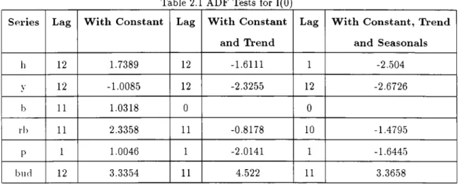
It is clear at first sight from the graphical representation that the series h, bud, p. b. rb and y are not stationary (Graphs 1-6). Unit root test is necessary in order to identify the order of integration of each individual series. For this purpose, the .Augmented Dickey-Fuller testing procedure which is based on Dickey-Fuller (1981) and described in chapter 3 section 2 is used. The results are reported in Table 2.1 through Table 2.3 in Appendix A.

The different ADF values with constant, constant and trend and constant, trend and 11 seasonal dummies are reported. The ADF test results with constant is

considered for a base line modelling. The other values are tabulated as further information for the readers. The lag length is specified according to the general to simple method (Ng and Perron (1995)). We begin from 30 lags, then the last signihcant lag is specified as the lag length and the matching ADF value is reported.

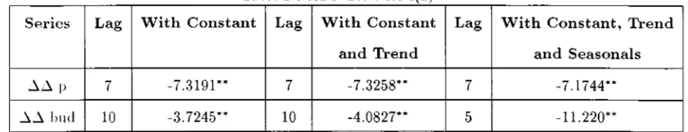
The ADF test statistics support the graphical results, that is the hypothesis of a unit root in each series is not rejected. So, all the variables are not 1(0) in 1% significance level, while the first differenced series of h, b, rb and y do not exhibit a unit root at 5%. The second differences of bud and p do not exhibit a unit root at 1%. Therefore, according to the ADF test results, we can conclude that h, b, rb and y are 1(1), and bud, p are 1(2). The graphs of the series are presented in Graph 1 through 6. The nonstationarity of each series and its order of integration can also be observed from the graphs.

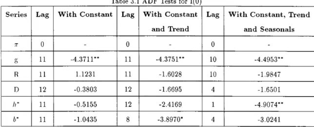
Considering the model presented in chapter 3 and the macroeconomics of the I’urkish economy, the variables that will be used in the regression analysis are tt ,

D. R, g, h* and b*. The first four variables were already described in chapter 4 and the last two ones stand for the log of ^ and ^ respectively. We should note that the variable K (the growth of financing instruments H* and B*) is not included in the regression and instead h* and b* are added. This is because we want to assess the direct effect of the base money and stock of bonds on inflation rather than the ('ffect of the growth of financing instruments on inflation.

Investigating the degree of integratedness of these variables using the ADF test witli the same procedure that was described in the first part of this section, we find

that g is 1(0), whereas tt , D, R, h* and b* are 1(1). More detailed results are reported

in Table 3.1 through Table 3.2 in Appendix A. The graphs (Graph 7-10) of these variables reported in Appendix B, support the ADF test results. From the graphs w(' can see that only the growth rate of real income is stationary whereas the other \ ariables should be differenced to make them stationary.

5.3

Results of Cointegration Test

This subsection tests for cointegration among the series ( tt , D, R, g, h*, b*). The first step is to apply appropriate differencing to the variables so that we can reduce the system to an 1(0)-1(1) system. At this point, we should note that the variables need not be of the same integration order and it is sufficient for them to be of order 0 or 1 to be integrated in the cointegration analysis. This results from the fact that 1(0) and 1(1) series, together, are assumed to behave nicely. In our case, applying differencing is not necessary because all the series are either 1(0) or 1(1).

In order to test for cointegration in the vector autoregressive model, VAR, the maximum likelihood procedure developed in Johansen (1988) and Johansen and Juselius (1990) is used. The system used is a first order vector autoregression with a constant term and a trend. The constant is entered unrestrictedly while the trend is restricted to lie in the cointegration space. Since the cointegration results are very sensitive to the lag length of the VAR, we will base our selection of the lag length on the Schwarz and Hannan-Quinn criteria. We start with a VAR(5) and reduce the lag length by one in a time, then the Schwarz and Hannan-Quinn test values for each system is obtained. We start with a VAR(5) because the used computer package program PcGive Professional 8.0 (1994) developed by Doornik and Hendry

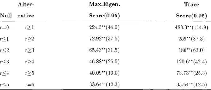
does not manage a higher lag length. The results reported in Table 4 show that the smallest value is associated to a V A R (l), therefore the optimum selected lag number should be one.

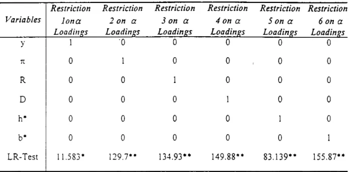
The cointegration results are reported in Table 5. Two statistics are reported to decide on the number of cointegrating vectors, these are the trace and the maxi­ mum eigenvalue statistics. Looking at these statistics leads us to accept definitely six cointegrating vectors for both of the tests (this is not a surprising fact if we con­ sider the parallel movement of our series which can be observed in Graphs (11-16).

The six rows of the standardized /5 eigenvectors report the estimated cointegra­ tion vectors as representative of the cointegration space. The standardized loadings presented by the a coefficients are all different from zero, which shows that there is a feedback process between all the variables. This clearly implies that no variable is weakly exogeneous for the parameters of interest (tests for weak exogeneity will be carried on in the next section).

If we drop the variables with small coefficients (smaller than 0.01), the following long-run relations are obtained from the standardized eigenvectors:

7T = R D -0.3387r + 0.114/i* (1) 0.017R-l-0.026L>-0.06/i* + 0.0116* (2) -0.31^ - 2.7l7T -b 0.603T> - 1.626* + 0.0636* (3) 19.24i7 + 8.7l7T - 1.5R + 21.996* + 5.466* + 0.12t (4) -0.16^ + 5.437t -1- OAR + 0.74T» + 0.576* (5)

b* = 2.01^ + 2.047t + 0.09i? + 2.88i:» - 2 .2 5 /1* + 0.03i (6)

Our interest is focused on equation 2 which is an inflation equation. This relation shows that inflation is little explained by our variables of interest, given the small coefficients associated to them as well as the wrong signs of some variables such as the sign of the scaled base money h* and the interest paid (R) which are expected to be positive and negative respectively.

5.4

Results of Weak Exogeneity Test

ill order to conduct a reliable single equation analysis, weak exogeneity of the vari­ ables should be tested. In accordance with the economic framework, all of the variables D, y, R, h* and b* should be weakly exogeneous for inflation (the parame­ ter 7t) and the other parameters in the inflation equation that were obtained in the economic framework section. That is knowledge of tt is not required for inference on the marginal processes of D. y, R, h*, b*.

A necessary condition for these variables to be weakly exogeneous for the pa­ rameters in the inflation equation is that the corresponding a loadings obtained in the cointegration analysis and reported in Table 5 are zero. But, as we have noted earlier, in the previous section, the a coefficients corresponding to all of the vari­ ables are significantly different from zero. This result leads us to reject the weak exogeneity hypothesis for the variables of interest.

-Another test based on the Johansen (1992a ; 1992b) procedure is also used to test the w’eak exogeneity hypothesis for all the conditional parameters. The procedure restricts the loading coefficients of the parameters and tests the restriction for sig­

nificance by an LR-test. For every parameter the restriction consists of imposing a matrix of a ’s in which the parameter in question has an a equal to one, whereas the remaining parameters have a ’s equal to zero. The test results, which are reported in Table 6 in the table appendix, show that the null hypothesis (D, y, R, /i*, fe* and 7T are weakly exogeneous in the inflation equation) is rejected with LR-tests of x(5) equal to 149.88, 11.583, 134.93, 83.139, 155.87 and 129.7 respectively. These test values are high enough to reject the null hypothesis

Satisfactory models should have regressors which are at least weakly exogeneous. If this is not the case, then these variables are considered to be endogeneous, that is a feedback exists between them. The lack of weak exogeneity and the presence of a feedback in the cointegrating vectors invites us to model a simultaneous equation system. However, it should be noted that lack of exogeneity does not necessarily require a simultaneous equation model. Rather, it implies that inference about the cointegrating vectors is performed better and easier at the system level (Metin 1996). Therefore, having estimated the cointegrating vectors in the previous section, it is possible but not very safe to proceed by single equation modelling.

Single equation and system of equations modelling will be the issue of the following ch apter.

6

EMPIRICAL MODELLING

In this chapter, two models are developed and implemented. The first is a condi­ tional single equation model based on a general autoregressive distributed lag (ADL) model. The second one is a VAR model consisting of the system of the six variables considered throughout this work.

6 ·!

Single Equation Analysis

In this section a general autoregressive distributive lag model is developed using a modelling approach from general to specific. Single equation modelling starts with an unrestricted sixth order general ADL model given below,

/i / — a' + ^ /32iDt-i + ' ^ /3siRt-i + ' ^ (34igt~i + ' ^ + l3eibf_i + ut

t = l i=0 i=0 t=0 t=0 t=0

where a represents the constant term and trend. The length of the lag is chosen as six because first, a higher lag would result in a significant loss of observations, second, the computer package program used and stated earlier does not manage a higher lag.

From the results of the extensive literature that has estimated inflation (eg: Metin(1995, 1996)), the signs of the coefficients are expected to be as follows:

/3ii, ,i = 1, ...,6 > 0 /?2i, ,« = 0, ...,6 > 0

= 0, ...,6 < 0 ,« = 0, ...,6 < 0

/3si, ,1 = 0, ...,6 > 0

/?6i, ,г = 0,...,6 > 0

These expectations imply that there is a positive relationship between inflation and its past lags, the scaled budget deflcit, the scaled base money and the scaled bond stock. Also, they imply that there is a negative relationship between inflation and the scaled interest paid and the growth rate of real income.

The model is fitted to our monthly data for the period 1986(1)-1996(12), then reduction based on Hendry(1988) general to speciflc simpliflcation methodology is made by eliminating, step by step, the statistically as well as economically most in­ significant regressors. The decision on which insignificant regressors are eliminated is based on three criteria:

1- The t-statistic is the criteria that is used in reducing the ADL model. The regressors that have a t-statistic lower than the critical one (1.96) are considered to be insignificant.

2- By developing the correlation matrix, the variables which are highly correlated are detected. And during the elimination process, one of these variables should be completely eliminated, because it is assumed that highly correlated variables hide the significance of each other. So, by eliminating one of them, the other variable may turn to be significant in the following estimation.

3- Eliminating the insignificant regressors with a higher lag length is preferable even if their t-statistics are higher than the insignificant regressors with a lower lag length. The reason is that the regressors which are nearer in time to the dependent ^^ariable are assumed to have a stronger impact that can be hidden by the presence

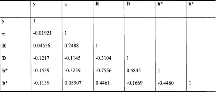
The correlation matrix for the variables Ap, D, g, R, h* and 6* is shown in Table 7 in Appendix A. The matrix shows that R and h* are negatively highly correlated with a correlation coefficient equal to —7.556. Also, D and /¿*, R and 6*, 6* and can be considered highly correlated with correlation coefficients 0.4845, 0.446 and -0.446 respectively.

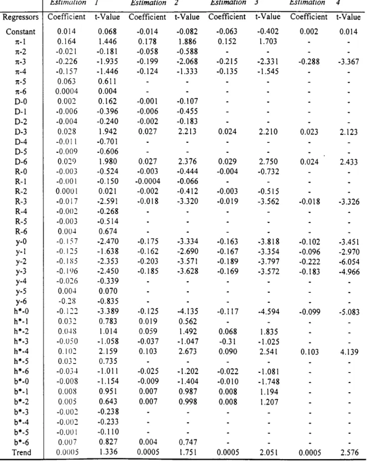
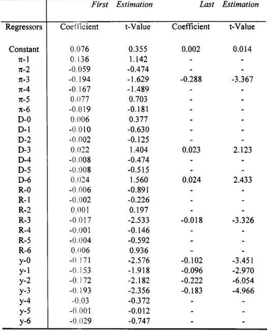
Applying a general-to-specific reduction process to the general ADL, a model of inflation is obtained. The estimation results and the reduction process are reported in Table 8 in Appendix A. The last remaining equation is given below,

TTt — 0.002 — 0.37T^_3 + 0.02Z)i_3 + 0.024Z)^_6 — 0.02i?^_3 — 0.1^^ — 0.1^i_i — 0.22^^_2 —

- O .U * + 0.U*_4 + 0.0005i

= 0.37,(7 = 0.022

All the explanatory variables have significant coefficients. This conditional infla­ tion equation shows that inflation is determined mostly by the growth rate of real income with a lagged effect and the expected sign. That is an increase in the growth rate of real income and its three first lags is expected to decrease inflation.

of the other variables.

Also, we assess a positive relation between inflation and the third and sixth lags of scaled budget deficit, but with a moderate effect. Monetization of the economy has a significant effect on inflation with the current scaled base money and its fourth pc'riod lagged value. However, it should be noted that the current scaled base money has the wrong sign. Surprisingly, there is a negative relation between inflation and

its third lag. The negative sign associated to the scaled interest paid regressor is an expected sign. An observed increase in the lagged interest payments, make people delay their consumption to buy government bonds. Therefore, price levels are ex­ pected to decrease, which in turn is expected to decrease inflation.

Eventhough the model has a very small standard error (cr=0.022), it is not con­ sistent with the theory especially that it significantly rejects the scaled bond stock variable h* as a regressor. We can conclude, then, that our findings do not support the theory. That is, inflation is not related to the stock of bonds issued, and is affected only by money financing.

The conclusions that can be drawn from the model are first, that the effect of budget deficits on inflation is not quick since the economy needs three periods of time lag to adjust inflation to the increases of budget deficit. Second, the results related to the scaled base money and stock of bonds imply that inflation is incurred solely by money financed deficits rather than bond financed deficits, which is a result found by many researchers (Langdana (1990), Scarth(1987), Sargent and Wallace(1981)) who sliowed that bond financed deficits are less preferable than money financed deficits. And, that this results in debt monetisation which, according to the monetarist view, will produce high inflation due to the higher rate of money growth.

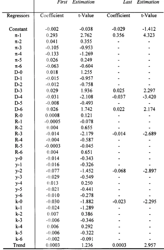
Two other single equation analyses with different combinations of the regressors including the variable K (growth of financing instruments) have been carried out and reported for the reader in Tables 9 and 10 of Appendix A. Noting that K is 1(0), the two single equations estimated are as follows.

= a + E A ^ ß2iDt-i + ^ ßsiRt-i + ^ ß4idt-i + ^ ßbiRt-i +

¿=1 ¿ = 0 2 = 0 2=0 2 = 0

6 6 6 6 6

~i = ö; + E

+ E

+ E Äi-Ri-j + E

ß‘ii9t-i

+ E

ß^iK-i

2

=

=

=

=

=

+ E

ß^iK-i

+ E

+

Ut

¿=0 ¿=0

These two regressions performed badly in terms of the signs of the coefficients associated to the significant regressors retained and, with respect to the regres­ sion reported earlier. For this reason, they were not chosen as the model explaining inllation variation (more details are reported in the Tables 9 and 10 in Appendix A).

As we have noted in chapter 5 section 4, a system in which weak exogeneity is rejected is better estimated by a VAR model than by a single equation. So, in the next section a simultaneous equation system is modelled.

6.2

V A R Model

The vector autoregressive (VAR) methodology has recently been used to estimate inflation and evaluate disinflation programs in countries with chronic high inflation (L·ciderman(1984), Dornbusch et al.(1990)). The reason behind the excessive use of this methodology is that it allows determining the joint stochastic behavior of the variables of a time series data, and therefore detects the dominant pattern of dependence between the variables.

In contrast to the single equation model, the VAR model does not require a pri­

ori assumptions when specifying the equations. Because the VAR methodology is

an econometric technique with no specific economic theory and allows for an un­ 34

restricted pattern of interdependence. But, this method is not completely free of restrictions. The choice of a specific variable ordering and the length of lags imply restrictions on a VAR system. The ordering and length of lags of the variables used in a VAR model should be specified before it is estimated. There is no specific way for choosing the ordering and the length of lags but two criteria known as the Scliwarz and Hannan-Quinn criteria can be used to compare the alternative ordering and lag structures.

As we have found in chapter 5 section 3, the Schwarz and Hannan-Quinn criteria suggest modelling a V A R (l) system where the ordering of the variables is reasoned by that the policy variables should come first. The system of equations that is estimated is given below:

Dt K K Rt 9 t T^t Dt-\ + + ^ * - 1 + Rt — 1 + gt-\ + TT^-i + Ut + Rt-\ + ^*-1 + Rt-\ + 9t-\ + 7T^-i + + Di-\ + + Rt-\ + gt-\ + TT^-i + Ut Rt-\ + Dt-\ + + gt-\ + TT^-i + Ui gt-\ + Dt-\ + ^ i _ i + ^ * -1 + Rt-i + + '^t + Dt-\ + /i*_i + + Rt-\ + gt-i +

The results of the estimation of this system are reported in Table 11. If we reduce the V A R (l) by eliminating the statistically insignificant regressors applying the same criteria that were applied in the previous section, we are left with the following system.

A = 0.63 + 0.58A-1 + 0.154/i*_i (1)

h;

b; = -5.52 + 0.466;_1 - (3)

A = -7.78 + 0.3 A - 1 - - 1.03^^ - 1 (4)

gt = 0.389 - 0.33iTt_i + 0.076/i*_i (5) Tt = 0.029 + 0.357rt_i (6)

Equation 1 shows that scaled budget deficit is positively related to its own first lag and to the first lag of scaled base money. This result is not an expected one, because increases in budget deficits should result in increases in base money and not vice-versa, given that budget deficits are financed partially by issuing money. The scaled bond stock variable was eliminated in the reduction process because it turned out to be insignificant, and since it is highly correlated with the scaled base money variable, its elimination was permitted.

Equation 2 implies that the scaled base money is positively related with its own first lag and the first lag of both scaled budget deficit and growth rate of real in­ come. Scaled base money is highly affected by its first lag, given that an increase by 1 percent in the current year’s amount of money issued is expected to increase the next year’s amount of money issued by 0.8 percent. The sign associated to the inflation in the scaled base money equation is negative, showing that an increase in this year’s inflation is expected to decay the next year’s growth of money issued by 91%.

The scaled stock of bonds equation, equation 3, shows that next year’s amount of lionds issued is expected to increase when current year’s amount of bonds is raised. Also, it is expected to decline if the amonut of money issued this year is increased.

Equation 4, shows that the amount of scaled interest paid is positively related to its own first lag. Increases in the amount of money issued are expected to decrease the amount of interest paid. This result comes from the fact that the amount of bonds issued decrease with a rise in the base money, and the stock of bonds issued is positively related to the interest paid. A rise in the current growth rate of real income is expected to decrease next year’s amount of interest paid. Considering the positive relationship between real income and investment from the income iden­ tity, and the negative correlation between investment and real interest, the previous stated result is not a strange one.

In equation 5, growth rate of real income is found to be slightly related to the hrst lag of the scaled base money variable. It is also negatively related to its own lag. This result is not very surprising if we notice that growth rate of real income is a very fluctuating variable in the Turkish economy, so its sign is not well predicted.

The last equation, equation 6, is the most important equation in this system, l)ecause it is the inflation equation. This equation shows that inflation is related solely to its own first lag. The fact that current inflation is predicted by its own lag rather than the other variables, implies that a high degree of inertia exists. From equation 6, we can see that the degree of inertia is about 35%. In this case, inflation is said to have its own life being unresponsive to policy changes. Inertia reflects