A routing algorithm for low earth orbit satellite networks

A ВОиТІѢТО A L G O E I T H M F O E LO¥/ E A E T H

O EB I T S A T E L L I T E N E T ¥ / O E K S

A T H E S IS

ШВМ-TTSL TO THE DEPARTMEiN’T OF ELSCTE2GAL

ЕІЕОТЕОШСЗ ЕІШ Ш ЕЕВІ:‘О

НіШ THE іШ Т іТ и Т І DF SLIGIN12HH-H Α ΪΗ НОЗ-НН:::

О J’ Τ-Ή DHDOTESJHEHTí

НС-Е-Г0Е

A ROUTING ALGORITHM FOR LOW EARTH

ORBIT SATELLITE NETWORKS

A THESIS

SUBMITTED TO THE DEPARTMENT OF ELECTRICAL AND ELECTRONICS ENGINEERING

AND THE INSTITUTE OF ENGINEERING AND SCIENCES OF BILKENT UNIVERSITY

IN PARTIAL FULFILLMENT OF THE REQUIREMENTS FOR THE DEGREE OF

MASTER OF SCIENCE

By

Cantekin Dingerler

July 1995

τ κ 5 ^ 0 4 ùf3G ІЭ35 Ь.і ί·ρ ί О »1 i , · -J j J О . j

I certify that I have read this thesis and that in rny opinion it is fully adequate, in scope and in quality, as a thesis for the degree of Master of Science.

Assoc. Prof. Dr. Erdal Arikan(Supervisor)

I certify that I have read this thesis and that in my opinion it is fully adequate, in scope and in quality, as a thesis for the degree of Master of Science.

Prof. Dr. Erol Sezer

I certify that I have read this thesis and that in my opinion it is fully adequate, in scope and in quality, as a thesis for the degree of Master of Science.

4 · .

Aİsoc/Prof. Dr. Ayhan Altıntaş

Approved for the Institute of Engineering and Sciences:

Pi’OL· Dr. Mehmet

Director of Institute of Engineering and Sciences

ABSTRACT

A ROUTING ALGORITHM FOR LOW EARTH

ORBIT SATELLITE NETWORKS

Cantekin Dingerler

M.S. in Electrical and Electronics Engineering

Supervisor: Assoc. Prof. Dr. Erdal Arikan

July 1995

In this study, we consider the geometric aspects of low earth orbit (LEO) satellite constellations and investigate the performance of a satellite network that uses our proposed routing algorithm.

The optimum inclination and harmonic factor of rosette constellations are obtained by considering the minimum coverage radius of a satellite. Actual altitude is determined by this radius and the specified elevation angle. The algorithm uses the uniformity of the geometric structure to form a continuously connected group of nodes in the network which renders global intersatellite connectivity information insignificant. Each group, consisting of a node and its four neighbours, does not change with time and a stationary network structure is obtained by allowing each node to communicate only with its neighbours. Queuing analysis of the network is made for both packet and voice traffic. Simulation results are then compared to analytical results derived from uniform ciricl equal traffic distribution.

The proposed algorithm is simulated in a scenario in which sources, desti­ nations, and gateways on the earth form the global traffic. We examine the effects of such a distribution on the performance of the network.

Keywords : low earth orbit satellite systems^ rosette constellations, satellite networks, •performance analysis, routing

ÖZET

YERE YAKIN YÖRUNGELI UYDU AĞLARI İÇİN BİR YOL

ATAMA ALGORİTMASI

Cantekin Dinçerler

Elektrik ve Elektronik Mühendisliği Bölümü Yüksek Lisans

Tez yöneticisi: Doç. Dr. Erdal Arıkan

Temmuz 1995

Bu çalışmada yere yakın yörüngeli uydu takımlarının geometrik özellikleri ele alınır ve önerilen bir yol atama algoritması için bir uydu ağının başarımı ince­ lenir. Eşeğimli uydu takımlarının eniyi eğimi ve katsıklık bileşeni bir uydunun ka23İama alanının enküçük yarıçapı dikkate alınarak bulunur. Yükseklik ise bu yarıçap ve görüş açısının büyüklüklerine göre belirlenir.

Algoritma, uydu ağının geometrik 3'^apısmın düzgünlüğü kullanılarak, bir­ birlerine sürekli bağlantılı olan, uydu grupları oluşturmayı önerir. Böylece uydulararası bağlanırlık bilgisine ihtiyaç kalmamaktadır. Böylesine bir grup, bir düğüm ve onun dört komşusundan oluşur. Bu komşuluk ilişkisi zamanla değişmeyen bir ilişkidir ve söz konusu olan düğüm sadece bu dört komşusu ile haberleşir. Böyle bir uydu ağının kuyruk çözümlemesi ı^aket ve ses trcifiği için yaiDihr ve sonuçlar benzetim sonuçlarıyla mukayese edilir. Çözümleme yapılırken trafiğin düğümlere düzgün ve eşit olarak dağıtıldığı varsayılır.

Önerilen algoritmanın yeryüzünde oluşturulan trafik dağılımı için benzetimi yapılır. Bu şekilde oluşturulan bir trafik dağılımının, uydu ağının başarımı üzerindeki etkisi gözlemlenir.

Anahtar Kelimeler : xjere yakın yörüngeli uydu sistemleri, eşeğimli uydu takımları, uydu ağları, başarım çözümlemesi, yol atama

ACKNOWLEDGMENTS

I would like to thank Dr. Erdal Ankan for his supervision, guidance, sug­ gestions and encouragement through the development of this thesis.

TABLE OF C O N T E N T S

1 INTRODUCTION 1

2 THE BASICS OF CONSTELLATION GEOMETRY 5

2.1 Orbit P a ra m e te rs... 5

2.1.1 H e ig h t... 5

2.1.2 S h a p e ... 6

2.1.3 Coverage Radius and Elevation A ngle... 7

2.1.4 Visibility... 8

2.2 Constellations with Circular O r b i t s ... 9

2.3 Optimization of Constellation Parameters 11 2.4 Intersatellite Range . ... 13

2.5 Parameters of the Studied Constellation 13 3 THE ROUTING ALGORITHM 15 3.1 Description of the A lgorithm ... 15

3.2 Packet T ra ffic ... 18

3.2.1 Jackson’s T h e o re m ... 19

3.2.2 Application of Jackson’s T h eo rem ... 20

3.3 Voice T raffic... 23

3.4 S im u la tio n s... 24

3.4.1 Results; Packet T raffic ... 24

3.4.2 Results: Voice Traffic... 26

3.5 Effects of Larger Constellation S i z e ... 26

4 SIMULATIONS OF A PRACTICAL SCENARIO 28 4.1 Simulation M o d e lin g ... 28

4.1.1 Satellite N e tw o rk ... 28

4.1.2 Terrestrial N etw ork... 29

4.2 Simulations with the XY A lgorithm ... 32

4.2.1 Packet T ra ffic ... 32

4.2.2 Voice Traffic... 32

4.3 Simulations with the SP A lg o rith m ... 34

4.4 Comments on the O b serv atio n s... 36

5 CONCLUSION 37 A Constellation Related Expressions 38 A.l Trigonometric Relations for a Spherical T rian g le... 38

A.2 Intersatellite R a n g e ... 39

A.3 Triangular E q u id ista n c e ... 40

A.4 Multiple Visibility D etection... 40

A.5 Orbital Period Derivation 41

B The Conditional Probabilités 43

LIST OF F IG U R E S

1.1 The four- and six-neighbour c a s e s ... 3

2.1 A polar circular orbit 6 2.2 Circular and elliptical o r b i t s ... 7

2.3 Observer-to-satellite profile... 7

2.4 Elevation angle versus Rm a xfor different a l t i t u d e s ... 8

2.5 View of a constellation [ 1 ] ... 9

2.6 Polar view of a constellation... 10

2.7 An earth-track of a satellite on a circular orbit with ¡3 = 59.1° 10 2.8 Multiple visibility c a s e ... 11

2.9 Usage of spot b e a m s ... 12

3.1 Network l a y o u t ... 16

3.2 Connectivity profile... 18

3.3 The two-tandem net 19 3.4 Possible paths traversing a selected dow nlink... 23

3.5 Simulation results - Tp us 7 - ... 25

4.1 Address distribution of the messages generated at source 17 30

4.2 Connectivity matrix 30

4.3 Locations of the nodes of the network at i = 0 ... 31

4.4 Average rate of messages received by (0, 1) from its coverage area 33 4.5 Channel occupancies on the outgoing links of (5,0) 34 4.6 Channel occupancies of the links of (0, 1) ... 35

A.l A spherical triangle [ 9 ] ... 38

A.2 Auxiliary orbit parameters [1] ... 39

A. 3 Enclosure test [ 1 ] ... 41

B. l Possible paths for a message coming from right 43

LIST OF TABLES

1.1 System parameters of several proposed LEO/MEO systems . . . 2

2.1 Types of orbits with respect to a ltitu d e ... 6 2.2 Several single-visibility constellations... 12 2.3 Parameters of the 2 4 /6 /j co n stellatio n... 14

3.1 Network delays with the XY algorithm for uniform and equal traffic distribution... 25 3.2 Call rejection ratios with the XY algorithm for uniform and

equal traffic d is trib u tio n ... ■ . . . 26

4.1 End-to-end delays with the proposed algorithm for non-uniform traffic distribution... 32 4.2 Call rejection ratios with the proposed algorithm for

non-uniform traffic d istrib u tio n ... 34 4.3 Call rejection ratios with the shortest path algorithm for

non-uniform traffic d istrib u tio n ... 35 4.4 End-to-end delays with the shortest path algorithm for

Chapter 1

INTRODUCTION

Many developments have taken place in wireless communications, cellular sys­ tems being the most widely accepted and implemented ones at present. These systems work in principle by dividing the service area into macro- or microcells, with each cell using a different part of the frequency spectrum. Each cell’s ge­ ographic range is between one hundred meters and scores of kilometers. These systems are designed for land coverage only, and therefore, such systems fail to provide global connectivity.

A satellite-based communication system is a good way of covering every point on earth. It is supposed to give complementary service to existing ter­ restrial networks where coverage overlaps and is the only accessible wireless service where ground-based systems cannot reach. Thus, a satellite network with a true whole-earth coverage can provide worldwide connectivity.

With a view to achieving this aim, geostationary (GEO) satellites have been in operation for a long time serving as relay stations for TV ti’ansmission and telephony. Due to limited satellite population capacity of the GEO plane and long propagation delays induced during transmissions (fs 240 msec round-trip), lower altitude orbits (LEO) are better suited to the purpose of deploying such systems. Another shortcoming of GEO satellite systems is that they cover the earth most efficiently between latitudes ±71.

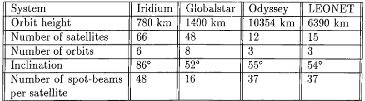
There have been several studies concerning the implementation of these systems such as Iridium [7], Odyssey, Globalstar, and LEONET [14]. All of them suggest partial or full usage of intersatellite links (ISL) for message trans­ portation. The interconnectivity is accomplished through the use of these links. 58-62 GHz spectrum is allocated by ITU to ISL operations [5]. Table 1.1 shows

System Iridium Globalstar Odyssey LEONET Orbit height 780 km 1400 km 10354 km 6390 km Number of satellites 66 48 12 15 Number of orbits Inclination 86° 52° 55° 54° Number of spot-beams per satellite 48 16 37 37

Table 1.1: System parameters of several proposed LEO/MEO systems

various parameters of these systems [14].

In this thesis, we investigate system parameters of a sample network con­ sisting of 24 satellites with 6 orbits and propose a simple routing algorithm, which we prefer to call ‘XY’ algorithm, that uses ISL. The satellite constel­ lation is designed to have continuous connectivity between adjacent satellites of the network. The XY algorithm makes use of this property for routing the messages. Therefore, global intersatellite connectivity information becomes in­ significant in the proposed algorithm. The price paid to achieve this is the higher constellation altitude but, as shown in Chapter 2, the change in the altitude is about 5.6% if the connectivity condition is restricted by direct line- of-sight. We analyze the network performance for both packet and voice traffic and make simulations to verify analytically predicted results. The performance measure is the average end-to-end delay for packet traffic and call-reject ion ra­ tio for voice traffic.

In optimizing the parameters of the sample constellation, we follow Ballard [1] rather than Walker [11]. The former optimizes the parameters to minimize the coverage radius of a satellite'while the latter optimizes the parameters to maximize the separation between satellites. The maximization of the separa­ tion between satellites is important when the interference problem is consid­ ered, however, it is possible to overcome this problem by technological means such as usage of spot-beams. The minimization of coverage radius implies a greater elevation angle which means a better satellite-user link quality. But, the value of the coverage radius is strictly geometry dependent, and hence the optimization of the geometry is carried out to minimize this quantity .

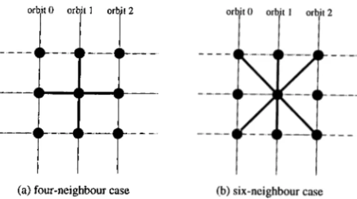
In our work, a node communicates only with its lour neighbours (Fig. 1.1(a)). A message is transported to its destination through the utilization of groups consisting of a node and its four neighbours. XY algorithm suggests

orbit 0 orbit 1 orbit 2

(a) four-neighbour case

Figure 1.1: The four- and six-neighbour cases

the use of a certain path among the possible paths between a source-destination pair. In earlier work, Wang [13] proposed a routing algorithm which did not limit the number of paths to a single one for a given source-destination pair and studied a six-neighbour case (Fig. 1.1(b)) for packet traffic. He showed by numerical results that the performance becomes 40% better than that of four-neighbour case for a constellation of 64 satellites with 8 orbits. In Wang’s study, the geometry of the constellation is not studied, and connectivity phe­ nomena is not mentioned. But the continuous connectivity requirement for a six-neighbour case forces the altitude of the constellation to increase further in comparison with a four-neighbour case (This increase is about 300% for the sample constellation in our study). Clearly, constellations with a large number of satellites enable the formation of groups with higher numbers of neighbours without significantly effecting the altitude much; however, the number of satel­ lites is limited by economic factors.

Each link in the network is modeled as an M / M / l queue. By letting each satellite generate Poisson traffic at the same rate, we analyze the queuing network assuming all links are independent of each other. We observe from the simulations that analytical results are close to simulation results in the case of packet traffic while they are not in the case of voice traffic.

A channel capacity allocation problem in LEO satellite systems is studied in [14]. In the study referred to, the shortest path (SP) algorithm is used for routing, and link capacities of intersatellite links, mobile user links, and gateway links are obtained. The traffic is distributed around the world in six regions (N.America, Europe, Asia, Africa, S.America, Australici). The intensity of the traffic is adjusted considering the possible number of users in those regions. The traffic is allocated to the different satellites according to their percentage of coverage of the respective land mass. Hence, the traffic in each region is assumed to be uniformly distributed over the area of that region. Two

types of connections are assumed in [14]; mobile-mobile and mobile-fixed. The capacities are obtained when routing is preferred to be accomplished through the use of (1) ISLs, (2) terrestrial networks (PSTN), and (3) a composition of ISLs and PSTN. Appropriate pseudo costs are assigned to ISLs and PSTN lines to make this preference in routing. Each satellite is assumed to have two or four ISLs which have to be turned on and off due to the interruption of direct line-of-sight between satellites.

We construct a practical scenario in which we model the traffic as discrete sources which are representatives of dense user population in various parts of the world. Therefore, non-uniform traffic distribution in a region may be modeled by altering the number of sources and the intensity of traffic at each source. We used 33 such sources plus 13 gateways as the interfaces of fixed- mobile traffic. We assumed that routing is accomplished through the use of ISLs only. We investigate XY algorithm and an other SP cdgorithm in which a satellite can communicate with any other satellite as long as they are on line-of-sight of each other. The flexibility in routing in SP algorithm reduces the propagation delay of a message compared to the one in XY algorithm: XY algorithm forces a message to make several hops to reach it destination while a message may reach its destination with one hop in SP algorithm case. But SP algorithm needs the information of link delays and the topology connectivity information in order to find the shortest paths between source-destination pairs. XY algorithm does not need such information.

We observe the effects of the non-uniform traffic distribution over the earth surface on the performance of the network in terms of the utilization of in­ tersatellite links and satellites themselves. Also the constellation geometry is important to determine the optimum utilization of the system.

All simulations are done with OPNET - a discrete-event driven network simulator - and results are given in the relevant sections of this thesis. The organization of the thesis is as follows;

In Chapter 2, geometrical properties of rosette constellations are discussed and optimum parameters for systems with single-visibility are obtained. In Chapter 3, using the proposed routing algorithm, the performance of the sam­ ple satellite network is analyzed and analytical results are compared with the simulation results. Simulations in which traffic sources are distributed on the earth surface, are described in Chapter 4. Final remarks cind conclusions are provided in Chapter 5.

Chapter 2

THE BASICS OF

CONSTELLATION

GEOMETRY

A satellite constellation is a geometric structure formed by a number of artificial earth satellites. What characterize a constellation’s geometry are the number and relative positions of the satellites in it. The number of satellites is chosen depending on the economic constraints, service type, and quality requirements. The positioning of satellites is dictated by the orbital properties.

The design of the orbits of the constellation considerably effects the service quality; therefore, understanding the mathematical background behind orbit generation is important. In this chapter, we investigate the geometry and properties of constellations with circular orbits.

2.1

O rbit P aram eters

2.1.1

H eigh t

One of the key parameters of an orbit is the altitude from the earth surface. There are altitude classes of orbits such as geostationary orbits (GEO), medium earth orbits (MEO) cirid low earth orbits (LEO). The ranges of these classes and their corresponding orbital periods are given in Table 2.1. The expression

Orbit type Altitude (km) Orbital period (hrs)

LEO 500 - 3000 1 .5 8 -2 .5 1

MEO « 10000 5.8

GEO « 36000 24

Table 2.1: Types of orbits with respect to altitude

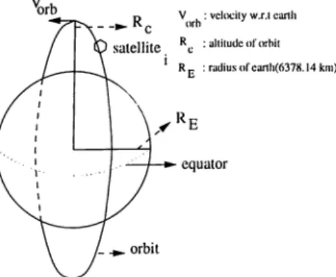
that relates period to altitude for circular orbits is obtained by using the grav­ itational force and centrifugal force balance at the satellite. Referring to Fig.

Figure 2.1: A polar circular orbit

2.1, the relation, which is derived in Appendix A, may be given as

R,

— = 0.795

Re

(2.1)

where T is the orbital period.

2.1.2

S hape

The orbits of a constellation may also be classified according to their physical shapes. Orbits can be either elliptical or circular (Fig. 2.2). Constellations such as Tundra have elliptical orbits while Iridium, Odyssey or LEONET have circular orbits [8]. The orbit shape is determined by the coverage properties of the satellite network.

It is stated in the literature that elliptical orbits are preferable for regional coverage while circular orbits provide more uniform coverage [1][11]· Therefore, constellations of circular orbits are more suitable for whole-earth coverage.

Equator

Figure 2.2: Circular and elliptical orbits

2.1.3

C overage R ad ius and E levation A n g le

Fig. 2.3 shows an observer-to-satellite profile.

Figure 2.3: Observer-to-satellite profile

In Fig. 2.3, the observer on earth is shown to be at the edge of the satellite covei’cige area. The constellation must provide this observer with a minimum elevation angle of (j) degrees during the communication with the satellite in view. The angle between the observer and subsatellite point subtended at the center of the earth must be at least Rm a x degrees to satisfy this requirement.

This angle is called the coverage radius of the satellite.

The elevation angle indicates how clearly a user may see the satellite in the least favorable coverage situation. As it is a measure of link quality and reliability, this value should be as high as possible. Proposed systems such as Iridium, Globalstar, and Odyssey have elevation angles of 8.2°, 20°, and 30° respectively [14].

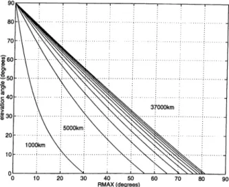
Figure 2.4: Elevation angle versus Rm a x for different altitudes

By applying the sine theorem to the EOS triangle, the expression relating coverage radius of a satellite to elevation angle and altitude becomes

tan (j) = cos - i j ^ )

sin Rm a x (2.2)

Rm a x is an altitude-independent parameter whereas elevation angle is not.

When Rm a x is determined, the elevation angle can be set to the desired value

by altering the altitude of the constellation (Fig. 2.4).

2.1.4

V isib ility

A whole-earth coverage guarantees that at least a certain number n > 1 satel­ lites are in view from any point on earth. Such a constellation is said to provide

n —tuple visibility. As n increases, the total number of satellites in the network

must also increase.

It is clear that there are trade-offs between altitude and elevation angle and between order of visibility and total number of satellites. The altitude of the constellation must be kept as low as possible to decrease propagation delay while larger elevation angle requires higher altitude. Obviously, a large number of satellites means a better performing system but the number of satellites is limited by such economic factors as installation and maintenance costs.

In this thesis, LEO constellations with circular orbits and single visibility

Figure 2.5: View of a constellation [1]

2.2

C on stellation s w ith Circular O rbits

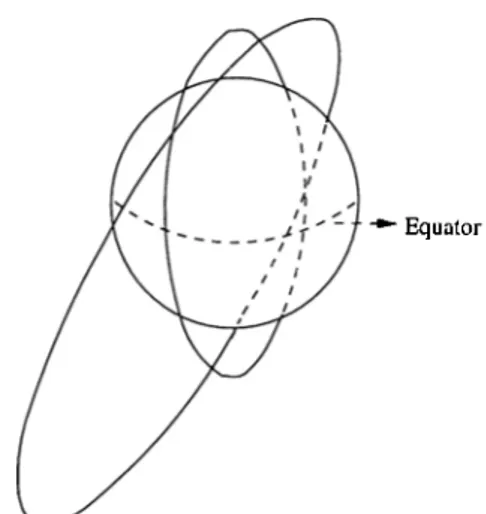
Fig. 2.5 shows a pair of satellites and their orbits. In that figure, H is the altitude of the constellation, and the orbits lie on the planes of great circles. The position of a satellite on this fixed celestial sphere can be described by three fixed orientation angles plus a time-varying phase angle:

ai : right ascension angle for the orbit plane

¡3i : inclination angle for the orbit plane

7i : initial phase angle of the satellite in its orbit plane at i = 0, measured from the point of right ascension

X = ^ t : time-varying phase angle for all satellites of the

constellation

When inclination angle is the same for all orbits, the constellation has a special name called ‘rosette’ [1]. This name has been chosen because the pattern of orbital traces when drawn on a fixed celestial sphere, resembles a many-petaled flower (Fig. 2.6). The expressions for the parameters defining the position of a satellite on the fixed celestial sphere (Fig. 2.5) are as follows:

27T ai = - p г ^ /2 7T . li = m Q — i . i = Q to N — I rn = (0 to N - 1 ) Q (2.3) (2.4) (2.5) where N stands for the total number of satellites of the constellation, Q for

Figure 2.6: Polar view of a constellation

the number of satellites in each orbit and P for the number of orbits of the constellation. Note that N = P Q. Given the orbit parameters, the earth-track of a satellite on that orbit looks like the one in Fig. 2.7.

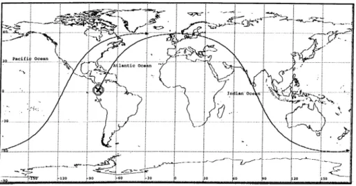
Figure 2.7: An earth-track of a satellite on a circular orbit with ¡3 = 59.1°

The factor m appearing in the expression for 7i is called the harmonic factor of the constellation. It influences the initial distribution of satellites over the sphere and is the precession rate of the constellation around the sphere. If m is a simple integer, the constellation has one satellite on each of N planes. If it is an irreducible ratio of integers, the constellation has Q satellites in each of the P planes, where Q is the denominator of m. Thus, shorthand notation

N f P f m may be used to describe a constellation completely.

Figure 2.8: Multiple visibility case

2.3

O p tim ization o f C on stellation P aram e­

ters

Optimization of parameters may be done in two ways: (1) to minimize Rm a x,

(2) to maximize Dmi n·, where Dmin is the minimum separation between any

pair of satellites during the precession of the constellation. The former method effects the elevation angle (Fig. 2.4), while the latter is important because it reduces the interference between satellite pairs. In both cases, harmonic factor

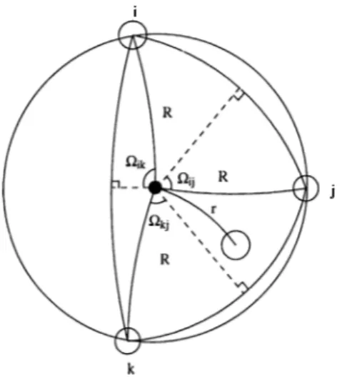
m and inclination angle /3 are optimized for the given N and P. Fig. 2.8 shows

a spherical triangle with the vertices being the subsatellite points (see Fig. 2.3 for the subsatellite points). A satellite’s coverage radius must be a.t least R degrees so that single visibility at the worst observation point, which is the center of the spherical triangle, is achieved. Observe that multiple visibility occurs whenever a fourth subsatellite point is inside the circle that encircles the triangle. Such cases are ignored in the optimization process since single visibility is sufficient. To detect multiple visibility cases, we need to know only whether r < R oi not. The expressions that give r in terms of R and intersatellite ranges are given in Appendix A.

Optimization procedure starts by choosing a parameter set {m, /3}. For this chosen set, [Rmax] is the radii set of the circles that encircle the nonoverlapping spherical triangles during the orbital period. RMax is the maximum of this radii set. For several combinations of different values for Rmox are obtained. Finally, the minimum of these RMax values is the Rm a x· Hence, optimum

parameters for the constellation with N and P are {rnopt,/3opt)·

The second way of the optimization method is straightforward and it needs only the calculation of arc length between pairs of subsatellite points with a set of Dmiti is the minimum of these values for each (m,l3) and Dm i n

is the maximum for m — niopul^ =

f^opt-Table 2.2 shows optimum parameters and corresponding Rmax £ind Dm i n

values for several constellations. It is observed that /3opt,R and ^opt,D are close in value for the 3 6 /6 /| constellation.

N m P o p t,R Rm a x j^opt,D DM I N

12 1/4 50.7 47.92 44.7 37.77

24 1/4 59.1 34.98 47.0 30.27

36 1/6 61.3 31.16 63.4 15.45

Table 2.2: Several single-visibility constellations

An empirical expression giving approximate values for Rm a x foi’ given num­

ber of satellites N and visibility number n is shown in [11]. It is derived by observing the actual values of Rm a x of numerous constellations and is given

as

Pn

R„

Rm a x,t

= 1 — pe— qn (2.6)

where p is the normalized value of Rm a x,uand is related to Rm a x,hthrough

the expression p„ = R M A X , n { ' ^ . It is stated in [11] that practical

values for q and p are 0.08 and 0.26, respectively. This makes pi = 1.31581

when n — 1. Rm a x values obtained from this expression for the constellations

of Table 2.2 are 43.53,30.78,25.13 when N=12, 24, and 36, respectively.

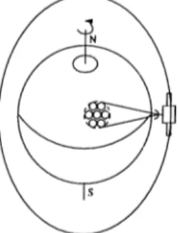
Figure 2.9: Usage of spot beams

It is possible to overcome the problem of interference by the use of spot

beams (Fig. 2.9) and frequency reuse concept while Rm a x is strictly geom­

etry dependent. In this thesis, optimum parameters enforced by Rm a x are

preferred.

2.4

In tersa tellite R ange

Intersatellite range rij, shown in Fig. 2.5, is the arc length between and nodes of the satellite network. The closed foi’m of the expression for Vij is given as follows [1] (Appendix A)

sin^ (rij/2) = cos^ ( ^ / 2) sin^ [(m -f l){j - i){Tr/P)] + 2 sin^ ( ^ / 2) cos^ ( ^ / 2) [m{j — i){'K! P)]

+ sin'· {^¡2) sin^ [{m - l)(j - i){Tr/P)] + 2 sin ^ (^ /2)co s^ (^ /2)sin^ [(j -i){Tr/P)]

cos [2a; + 2m(j + ¿)(7r/P )] (2.7)

Intersatellite range is useful to determine the maximum arc length possible between any two satellites. When -^rij{t) = 0 is solved, we obtain tm = ^ m(jp)T |,j^g time when the maximum arc length occurs between nodes i and j . Evaluation of rij at time tm gives

ra \t=tm = 2 arcsin

+ 2sin^(;5/2) cos^(^/2) sin^(

P m{j — i)TT,

)

-f 2 sin^(^/2) cos^(/3/2) sin^(

P )

U - 0 nl/2' _(2.8)

This expression implicitly influences the height of the constellation as shown later.

2.5

P aram eters o f th e S tu d ied C o n stella tio n

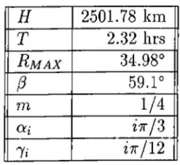
The 24/6/^ pattern is the constellation we have chosen for our studies. Below are the parameters of this structure with the elevation angle (j) being 10°. Note that all values are obtained without taking into consideration the oblateness of the earth.

From Table 2.2, Eqs. 2.2-2.5, the following parameters are obtained: H 2501.78 km T 2.32 hrs Rm a x 34.98° /3 59.1° m 1/4 Oii li ¿7t/12

Table 2.3: Parameters of the 2 4 /6 /j constellation

C h a p ter 3

THE ROUTING

ALGORITHM

In this chapter, the description of the proposed algorithm (XY algorithm) is given and network analysis is carried out for both packet and voice traffic. In the case of packet traffic, delay becomes the criterion for the performance of the network while call-rejection ratio is the performance measure in the case of voice traffic. A queuing analysis for network delay is given and then analytical results are compared to simulation results. For voice traffic, we investigate the expected call-rejection ratios when the network load is altered and compare these ratios with the simulation results.

3.1

D escrip tio n o f th e A lgorith m

Overall network layout may be viewed as a two-dimensional plane on which satellite nodes are placed on coordinates (xi,yi). The pattern repeats itself as a natural outcome of rosette constellations. Fig. 3.1 shows the network layout. Vertically aligned nodes represent the satellites on the same orbit, while each vertical line represents the orbits. Observe that a satellite in the layout has communication links with four adjacent nodes and is allowed to send its messages only on these links. For a system of A /P /m , the ¡position indexes of nodes adjacent to a given node at (.t,, ?/,·) and their corresponding

direction orientations are as follows: the satellite on the right is at position (3:(t'+i,modP)î î/î); the satellite on the left is at (^(¿-i.modP), 2/«)) the upper satellite is at (a;i, j/(i+i^niodQ))) and the lower satellite is at {xi,y(i-i,modQ))· We use the

O --- i >--- ( i--- i i--- i i--- i » i i--- f

(.0) (1 ()) (2 .0) (P- 1.0) ((,(

i --- i i--- i i--- i >--- i i--- i i--- 1

3) (1 .2) (1 ( C . l ) (1 .0) (1 (O.Q-l) (l.Q -l) (2.Q-1) ·-(0 3) (2 .2) (22) 1) (2,1) .0) (2,0) --- · — 3) (3 3) (4 2) (4 (O.Q-l) (1,Q-1) (2.Q-J) 3) (5 2) (5 (P-l.Q-1) (O.Q-l) • ---: nodes ■ : links (P-I.Q-1) (O.Q-l)

Figure 3.1: Network layout

terms rights left, up, and down instead of indicating the relative position indexes of adjacent satellites of a node.

The algorithm looks for the shortest path for routing, in the sense that the path has the smallest number of link traversals for a given source-destination pair. Clearly there is more than one such path but the XY algorithm chooses a certain one in accordance with certain preference rules described below.

Direction priority is one of the preferences: vertical direction has higher priority than horizontal direction, so vertical routing is accomplished first. An­ other preference is made whenever the destination is at the same distance from up and down or left and right. In the former case, going up is preferred white going right is chosen in the latter case. This strategy reduces the number of possible paths to one and a virtual circuit type of connection is established for packet traffic. This type of connection has the advantage of preserving the sequence of transmitted messages at the receiver node [10].

The following is an example demonstrating how these preferences are made: Assume node (2,1) has a message destined to (5,3). It must first be routed in the vertical direction, that is, it must reach the y = 3 level. But observe that the message can reach y = 3 with two links from either the upward or downward direction (remember that the pattern repeats itself). Going upward is preferred, so next node will be (2,2). Then (2,2) will forward the message to (2,3) and vertical routing is completed. Now, observe that the destination (5,3) is three hops away from (2,3) from left and right. Since going right is

preferred, the message is forwarded to (3,3). It is then sent to (4,3) and finally to (5,3). The whole path is indicated with dotted lines in Fig. 3.1.

Formally, to route a message with the destination address {xdst, Vdst), a node at (xseif,yseif) rnakes the following routing decisions:

S te p 1. Check whether pdat = Vseif and Xdst = Xseif- If true, go to Step 5.

S te p 2 . Determine whether vertical routing is completed. If tjdst = Vseif go to Step 4.

S te p 3. Obtain vertical distance as Vd = Pdst — Vseif- If (lurfi < Q!2)

If {vd > 0), forward it to {xseii-,y{seis+i,inodQ)), go to Step 5. If (vd < 0), forward it to (xseif,y(sei/-i,modQ)), go to Step 5.

H(lvdl = Q/2)

Forward it to (xseif,y(seif+i,modQ)), go to Step 5. If (lurfi > Q/2)

If (Vd > 0), forward it to (Xaelf,y(sel/-l,modQ)), gO to Step 5.

If (vd < 0), forward it to (xseif,y(seif+i,modQ)), go to Step 5. s te p 4. Obtain horizontal distance as hd = Xdst ~ Xseif-

If {\hd\ < P/2)

If {hd > 0), forward it to {x(self+l,modP),yself), go to Step 5. If ( h d < 0), forward it to ( x ( a e i f - i , m o d P ) , y s e t f ) , g o to Step 5.

If (\hd\ = p /2 )

I'OlWaid it to (x (^sel f d-l, modP) i y sel 1 gO to Step 5.

If (|/id| > P /2 )

If {hd > 0), forward it to {x{seif-i,modP),yseij), go to Step 5. If {hd < 0), forward it to {x{seif+i,modP),ysetf), go to Step 5. s te p 5. End

To communicate with the four adjacent satellites, ci node must be connected to neighbouring nodes at all times. Two nodes are assumed to be connected when there is a direct line-of-sight (LOS) between them.

As the altitude of the constellation is fixed for all orbits, the criterion for connectivity can be stated as {If + P^;) cos(() > Pp (Fig. 3.2) since the earth is assumed to be a sphere. The equation implies that the minimum possible altitude is determined by the largest arc between the two adjacent satellites.

We need to trace intraorbit and interorbit distances to determine the max­ imum arc possible. Intraorbit distance is constant at all times and for 2 4 /6 /|

Figure 3.2: Connectivity profile

pattern it is equal to 27t/4 = tt/2 (evenly spaced four satellites on each orbit). Interorbit distance is time-dependent as stated in Eq. 2.7 and the maximum of this quantity may be calculated by Eq. 2.8. The j — i expression in Eq. 2.8 is equal to one for adjacent nodes on adjacent orbits. It turns out that the max­ imum intersatellite range for right/left neighbours in a 2 4 /6 /1 constellation is 68.8°. It is clear that intraorbital separation of 90° determines the minimum altitude of the constellation. We obtain H > 2641.91 km from the expression cos(7r / 4)(jff -|- Re) > Re «md take H -(- Re = 9050 km in our study. The or­ bital period becomes 2.3844 hrs by Eq. 2.1 and the elevation angle increases to » 1 2 °. These values are used while analyzing the proposed routing algorithm. Since the optimum inclination angle is independent of altitude, it remains as

/3 = 59.1°.

3.2

P acket Traffic

For a network of size P * Q (Fig. 3.1), let us define a parameter В which stands for the diameter of the network [12]. This diameter indicates the maximum number of hops that a message makes to reach its destination. It is seen that В = Bx + By \i Bx — [P/2J and By = [(^/2j, where Bx,By represent the maximum number of hops in x and у direction, respectively. Given the maximum number of link traversals, expected number of hops in x dimension may be obtained as follows:

TX

avg = Y^ kP r{ k )

k=0

(3.1)

■ ' ^2 -m n i-O

---(lUCllC ---^ (lUCUC ---- ^

Figure 3.3: The two-tandem net

where Pr(Â:) is the probability that a message traverses k links to reach its destination.

Pv(k) is related to the number of nodes that can be reached by a given

node through k link traversals. Under uniform traffic, the explicit expression for Eq. 3.1 is = = o i + l | - f 2 | - f . . . - b ( P / 2 - l ) | + ^ ^ k=0 P

P

T ’

L a v g — ^ (3.3)

P f i + Q f i , P, Q even P/A -b — l)/AQ , P even, Q odd (p2 _ 1 )/4 P + (Q2 _ i)/4 (5 ^ Q

(P^ — 1)/4P -b Q/4 , P odd, Q even

We observe that the average number of link traversals for the case of 2 4 /6 /1 is 2.5 hops.

3.2.1

Jack son ’s T h eorem

Jackson’s theorem may be used to model a multiple-resource network as a queuing network. Fig. 3.3 shows a simple open network of tandem queues.

Referring to the figure, Jackson’s theorem states that the equilibrium prob­ ability, Pr(A:i,A:2), of finding ki customers in the first node and k^ customers in the second node is given by

Pv(ki,k2) = (1 - p i ) p ^ ' ( l - p2)p2^ (3.4) where pi —_{r* Hi}

This equation is simply the product of the state probabilities for two in­ dependent M /M /1 queues. From the Burke’s result [6] that the output of an

M / M / l queue is a Poisson process, any feedforward network of exponential

queues that is fed from independent Poisson sources, generates an independent arrival process at each node which is Poisson. Therefore, assuming the service time is chosen independently and exponentially at each node, the joint proba­ bility distribution over all nodes is the product of marginal distributions each of which is the solution to an M / M f l queue [6]. Kleinrock suggests to use this theorem even if the service time is not sampled independently at each node

[Kleinrock’s independence approximation) [2]. This approximation lets us to

express the total average delay of a message traversing a path p as the sum of individual delays at each link through the whole path as stated in Eq. .3.5.

Tp = _{E ( l i + T.)}

all links on path p

(3.5) where Tg is the average queuing delay and Tg is the average service delay at each link. Individual delays (queuing -f- service) may be found by using the average delay expression for an M/ M/ l queue

T = (3.6)

A

where p is the service rate and A is the arrival rate to each link.

We define R = [vij] as the N x N transition probability matrix such that

rij is the probability that a message, after receiving service at node i, goes to

node j . Therefore, the probability that a message leaves the network at node i is 1 — rij. The total (internal -f external) arrival rate of customers to

the i*^ node is defined to be Xi. To find Ai, we must solve the linear equations of the form

N

Xi — ,7i + X) ^ (3.7)

where 7i represents the external arrival process rate to node i. If we denote A = [Ai, A2, · · ·, A;v] and 7 = [71, 72, · ’ ’ ) 7n], then the equation above becomes

A = 7 + AR (3.8)

When A is known, arrival rates to each link can be calculated and hence, the delay in Eq. 3.5 can be obtained.

3.2.2

A p p lic a tio n o f Jack son ’s T h eorem

This theorem may be applied to the network in Fig. 3.1. We need to find R in order to find aggregate arrival rates in Eq. 3.8 for given 7 . There may

be four transitions from each node: up(u), down(d), right(r), and left(l). Let

P{D'^ = w) be the probability that the message departs from the present node

on link w and P{D~ = w) be the probability that the message arrives at the present node on link tn, where w G {u ,d ,r ,l,e } . D~ = e means the message enters the network from the present node and D'^ — e means the message exits the network from the present node. Then, transition probabilities may be written as follows:

P{D+ = w ) = = v)P {D - = v) (3.9)

Not all terms in the above equation are accounted for in the calculations of transition probabilities. The reasons for this are that a message is not permitted to go to the direction it comes from (v ^ w in Eq. 3.9) and that the algorithm prefers certain routing directions as stated earlier (e.g., a message cannot go up/down if it has come from left/right because moving in horizontal direction means vertical routing has already been completed). It should also be noted that a message coming to the present node from its lower adjacent can also be seen from that adjacent node as going up {P{D'^ = u) = P[D~ = d)). The same analogy applies to other directions as well. Schematic solutions to conditional probabilities in Eq. 3.9 are given in Appendix B. Transition probabilities for a 2 4 /6 /j constellation with uniform traffic distribution cire:

P(D+ = u) = ZP{D- = e)/4, P(D+ = d) = P{D~ = e)/4, P{D+ = r) = P {D - = e), and P(B+ = 1) = P {D - = e)/2.

The last equation to solve for all the probabilities is

P{D ^ = io) = l

wE{u,d,r,l,e]

(3.10)

from which we have P{D = e) — 2f7,P(D '^ = u) — 3/14, P{D'^ = d) = 1/14, P{D+ = r ) = 2/7, P{D+ = /) = 1/7· Observe that P(T>- = e) - 2/7

may be found by considering the average number of hops that a message makes. As has been shown earlier in this chapter, average number of hops for 24/6/1 structure is 2.5. Each generated message then, contributes to the transit traffic of the network by 2.5 messages. Each message also contributes to the traffic of the node it is originated, therefore, each message creates an effect as 2.5 + 1 messages are injected into the network. Then, the probability that a message is not transit is simply ^ which is the same as the result obtained above.

By inserting the transition probabilities in the matrix R and arranging the

Eq. 3.8, we obtain 0 ^0 1 0 ·· · 0 ^0,5 ^0,6 0 · · · 0 ^0,18 0 · · · 0 ^'1,0 0 n , 2 0 · · · 0 »'1,7 0 · · 0 _{n , 1 9 O ' O} R = - 0 · · · 0 »'23 ^5 0 · · · 0 _{^’23 ,17 ^23,18} 0 · · 0 ^'23,22 0 · · · 0 _ 0 P ( D + = r) 0 · · 0 P ( D + = 1) P ( D + = u) 0 · • 0 P ( D + = d) — P ( D + = 1) 0 P ( P + = r) 0 ■ ·■ 0 P ( D + = u) 0 · • 0 P ( P + = d) 0 · · 0 P ( P + = u) 0 · · 0 P ( P + = d) P ( P + = r ) 0 · ■•0 P ( P + = 1) • 0 • 0 \ = R)- 1 (3.11)

Assuming the external arrival rate is the same at each node of the network (71 = 72 = · · · = 7n = 7)) as expected, Ai = A2 = -- - = AAr = A and aggregate arrival rate to a node is

A = 3.57 (3.12)

Now that the aggregate traffic is known, delay may be calculated. To find individual link delays, we need to know the load distribution on each link. Load on each link is calculated by simply multiplying the probability that a message goes to that link by the arrival rate

Xw = XP{D'^ = w), w e { u ,d ,r j } (3.13) It is therefore seen that the links do not share the aggregate load evenly.

The average delay on the whole path is obtained by using the expected number of links that a message makes, in particular, the average hops it makes in each direction. = 1 is shared between the up and down directions as 0.75 and 0.25, respectively, and = 1.5 is divided as 1.0 and 0.5 between the right and left directions. Let Tup,Tdown,Tright,Tieft be average individual delays on corresponding links. Then, from Eq. 3.5, the average delay on path

p is

Tp — 0.75Tup + 0.25Tdown + ^•^Tright T (3.14) To include propagation delay in the analysis, we need to know total trav­ eled distance which may be obtained by summing the distances traveled in each direction. Distances in each direction are obtained by multiplying the expected number of hops by the average hop distance in that direction. In­ traorbit hop distance is fixed and equal to 2 sin(7r/4)9050 km for the 2 4 /6 /| case. Interorbit average hop distance is assumed to be the arithmetic average of the maximum and minimum separation distances. These values are given as 68.8° and 15.54° respectively when /S = 59.1°. The total average propaga­ tion delay then becomes Tprop ~ 73.3 msec. Finally, total average delay I'a is T -I- Tp \ -^prop·

I

Figure 3.4: Possible paths traversing a selected downlink

3.3

V oice Traffic

We may obtain the channel occupancy distribution of a link by counting the total number of paths which traverse that link. For example, choose the down­ link of node (0,1). Fig. 3.4 is the schematic representation of the paths that use the downlink of (0, 1) as a part of the whole path. We observe that there are six possible paths. In a similar fashion, we obtain 18,24, and 12 possible paths for an uplink, rightlink, and downlink, respectively. If each node gener­ ates 24 uniformly distributed calls, we expect that there is a session between every source-destination pair and we expect the occupancy to be 6,18,24,12 channels for down-, up-, right-, and leftlinks. So, we may write the call arrival rate to an uplink as

^ 18 37

“ 576^^'' “ -1 (3.16)

where 7 is the call generation rate per node. The other link rates are Xdown — 4,

Xr i ght ~ 7) X l e f t ^ ·

Once the rates are known, the call-rejection probability at each link may be calculated by Erlang B formula.

Vm,y ( \ h t n ml y = up, down, right, le ft (3.16) Recall that a message is expected to traverse 2.5 links consisting of a 0.75 uplink, a 0.25 downlink, 1 rightlink, and a 0.5 leftlink. The call rejection at a node hapiaens when the node cannot find a complete path to call’s destination. Then, the probability that a call request is rejected by a node is

Pr = 0.7bpm,up + 0.25^772, down T Pm,right T ^•^Pm,left

2^ (3.17)

This probability may be thought of as the average probability of rejection. The exact probability of rejection may be obtained as follows: we select cui arbitrary node and write rejection probabilities for paths to each possible des­ tination. For example, choose node (3, 2). One possible destination is (4,3) and the path to (4,3) consists of one uplink and one rightlink. Probability of rejection is 1 - (1 - pm,«p)(l - Pm,right)· If this procedure is repeated for all other nodes of the network, the desired probability may be obtained. Note that we

used Kleinrock’s independence approximation [6] in the calculations for both the exact and average probabilities; all links are assumed to be independent of each other.

3.4

Sim ulations

Simulations are performed for the 2 4 /6 /| constellation. In the case of packet traffic, we let each node in the network be a generator of packet traffic so as to produce a semblance of the external arrival process. Packet generation process is Poisson and packet sizes are drawn from exponential distribution with an expected size of 1024 bits. Propagation delays incurred during intersatellite transmissions are included in the simulations. Each node’s output links are assumed to have infinite buffer size and each link’s transmission rate is taken as 100 kbits/s.

In the case of voice traffic, we assume that call duration is exponentially distributed with an average of three minutes. Calls are generated by satellites and call arrival process is Poisson. Each link has 30 channels.

3.4.1

R esu lts: P acket Traffic

Several simulations are run for different 7 (external traffic injection rate/node) values. Table 3.1 shows average delays versus 7 with and without propaga­ tion delays for packet traffic. Observe that the propagation delay is about 85 msec which is about 12 msec moré than what we found in previous sections. This is mainly due to the approximation of average interorbital distance. Fig. 3.5 shows the plot of Tp (average delay without propagation delay) versus 7 together with analytically obtained values. We observe that the simulation results are very close to the theoretical results. Simulation results are not ob­ tained in the neighbourhood of saturation level because delay builds up as the simulated time advances. Nevertheless, the simulation results confirm that the network saturates at the analytical limit.

7 (packets/sec) Tp “1“ Tpf>Qp ^ms0c^ Tp (msec) 1.0 107.69 23.84 4.0 110.06 25.77 10.0 112.05 27.73 14.3 113.42 29.14 20.0 115.33 31.00 33.3 120.18 35.83 50.0 128.58 44.23 66.7 142.39 58.07 76.9 160.28 76.06 85.5 191.18 106.96

Table 3.1: Network delays with the XY algorithm for uniform and equal traffic distribution

Figure 3.5: Simulation results T p v s j

3.4.2

R esu lts: V oice Traffic

Table 3.2 shows the analytical and simulation results for the call-rejection ratio where 7 is the call generation rate of a node. Observe that average values are

7 (ca//s/s) Exact probability Average probability Simulation results 1.00 0.871 0.739 0.636 0.50 0.729 0.515 0.452 0.33 0.563 0.343 0.305 0.25 0.396 0.211 0.207 0.20 0.250 0.120 0.122

Table 3.2: Call rejection ratios with the XY algorithm for uniform and equal traffic distribution

close to simulation results when network load is low and exact probabilities seem to be quite different than simulation values; independence assumption seems to be failing. The reason is that all links on the path of an individual call work in a cooperative manner: when a session is initiated, every link on the path will allocate its resources and deallocate them when the session terminates. So, lirdi-by-link based analysis is not as valid as it is in the case of packet traffic.

3.5

E ffects o f Larger C on stellation Size

When 36/6/1 constellation is investigated, the aggregate rate can be shown to be A = 47 (Eq. 3.8). Therefore, saturation of the network is expected to occur at a relatively lower rate compared to the saturation level of 2 4 /6 /|. But, the size of the network is one-half the 2 4 /6 /j case and the external rate per node is assumed to be the same as 24 node model, which will not be the case in general. Usually, as the number of satellites increases, external arrival rate per node is expected to decrease since the geographic area span is smaller for each satellite.

For convenience, we reassert the assumption that the external traffic per node remains the same. This means external traffic is increased by 1.5 times. Observe, however, that the aggregate rate per node is 1.14 times the previous one (remember A = 3.57 24/6/^ case). This implies that the burden of each

node is lowered relative to the global message injection rate to the network. Another aspect of this constellation is the reduction of the propagation delays between satellites (fti 61.2 msec) and between earth and network due to the lower orbit altitudes. So, we may confidently say that the network performance improve as N increases.

Also related with the network size is the choice of P and Q. We have seen that with the proposed routing algorithm, links in different directions do not carry the same amount of traffic. This imbalance is due to the preferences made in the routing algorithm because of the asymmetric structure of the network. Observe that when Q and P are odd, there will be symmetry in the vertical and horizontal directions. If these quantities are odd and equal, the network is fully symmetric and each link will carry the same amount of load under uniform and equal traffic distribution assumption (consider the case of 25 satellites with 5 orbits). This is an advantage when link utilization is of concern, but in most cases the traffic distribution is not uniform and is not equally distributed among the nodes of the network. Real traffic may compensate for the imbalance providing a near-optimal usage of the network.

Chapter 4

SIMULATIONS OF A

PRACTICAL SCENARIO

Recall that the analysis in Chapter 3 depends on the assumption that the external traffic arrival process to satellites is Poisson and that traffic is equally distributed. This assumption seems reasonable in many cases but may not approximate an actual situation. It is obvious that in a global traffic network, a more detailed analysis must be carried out. In this chapter, we present detailed simulations integrating the satellite network with the earth traffic and observe the effects of a practical situation on the performance of the network.

4.1

S im ulation M od elin g

4.1.1

S a te llite N etw ork

The constellation that is used in our simulations is 24/6/^. The parameters of the constellation are the same as those in Chapter 2. Multiple access to the satellite network is assumed to be accomplished by other protocol layers. Source-destination satellites of a session are assumed to remain the same for the duration of the session. The simulations are done for both packet and voice traffic.

Two algorithms are employed for routing: the XY algorithm, which was described in Chapter 3, and the shortest path (SP) algorithm. In the shortest

path algorithm case, each node can communicate with any of the other satellites as long as they satisfy line-of-sight (LOS) condition (see Section 3.1 for LOS condition). The costs of the links are average link delays in the case of packet traffic and they are channel occupancies in the case of voice traffic. Link costs are updated once every 2 seconds in packet traffic simulations and channel occupancy information of any link is instantaneously updated in voice traffic simulations. The Bellman-Ford algorithm is used to find the shortest paths [10].

In the case of packet traffic, the transmission rates of output links for each satellite are 100 kbits/s and satellite input/output buffers are assumed to be of infinite size. The links have 30 channels for voice traffic. We assume that a circuit between a source-destination is set up instantaneously and channels on the whole path are allocated simultaneously.

4.1.2

T errestrial N etw ork

There are 33 nodes which are distributed on the earth surface and represent traffic sources. All source locations are fixed since their mobility is negligi­ ble compared to satellite network mobility. We include the effect of mobility by classifying the traffic generated at each node as (1) mobile-to-mobile, (2) mobile-to-fixed, and (3) fixed-to-mobile. We assume 30% of the messages are mobile-mobile, 35% mobile-fixed, and 35% fixed-mobile.

Whenever a traffic source generates a fixed-mobile message (source is fixed, destination is mobile), the message is first forwarded to the closest gateway station and then accesses to the satellite network. If the source is mobile, it reaches the satellite network directly. Similarly, if destination is mobile, the satellite network communicates directly with the destination. Otherwise, a gateway station relays messages from the satellite network to the fixed des­ tination. Therefore, we include 13 gateway stations as interfaces for fixed to mobile or mobile to fixed traffic in various parts of the world.

Packet and call generation process is Poisson. Packet sizes and call du­ rations are exponentially distributed with an average packet size of 1024 bits and an average call duration of three minutes. Destination of messages are generated according to predefined distributions for each source (Fig. 4.1). The simulation variable is the intensity of generated traffic at each node and is assumed to be the same regardless of time zone. This assumption may be justified if the worst scenario is in question.

F'igure 4.1: Address distribution of the messages generated at source 17

Connectivity information is updated once every 10 seconds. A square con­ nectivity matrix of size 33 -F 13 -|- 24 is maintained within the simulation. Fig. 4.2 shows the comiDonents of this matrix. A=[ajj] and aij — 1 when a satellite

C = “l *‘2 ■·· “24 .h h - ^33^1 h , ^13 “2 _{A B E} ‘*24 »2 / B 0 D ^33 g| S i t D E 0 S\3 u. satellites s: sources

Figure 4.2: Connectivity matrix

j is connected to i, otherwise it is 0. Submatrix A is constant in the case of XY

algorithm while it varies in the case of SP algorithm. We define what source belongs to which gateway; submatrix D is fixed. As there is no direct con­ nection among the gateways and among the sources, we put 0 in the relative positions in C. However, submatrices B and E change with time. Whenever a source or a gateway is in the coverage area of a satellite, bij — 1 or e{j = 1.

For simplicity, we assume that any ground node can reach only one satellite. This satellite is the one that has the closest subsatellite point to the ground node. Note that this provides a greater elevation angle for a user.

(L> ■s_c (U O <D XJ_o a S' & O (U ■§_(H <D *s_cd CO

Figure 4.3: Locations of the nodes of the network at i = 0

4.2

Sim ulations w ith th e X Y A lgorith m

4.2.1

P acket Traffic

In this simulation, we include the propagation delays between sources and gateways and between the earth and satellite network. We assume a constant propagation delay of about 1.86 msec between sources and their gateways. Average round-trip delay between earth and satellite network is about 26.6 msec. The average end-to-end delays for various traffic loads are given in Table 4.1. Although there are additional delays, we observe that packet delays

packets/s delay (msec)

10.0 87.9 3.33 84.3 2.00 83.6 1.43 83.4 1.00 83.0 0.5 82.9 0.2 80.2

Table 4.1: End-to-end delays with the proposed algorithm for non-uniform traffic distribution

are smaller than the results in Table 3.1. This decrease is due to address distribution of messages (Fig. 4.1). As short distance traffic is dominant, we expect a satellite to forward a message coming from earth, back to earth. This also implies that a larger amount of traffic can be handled because intersatellite links are not utilized as much.

We also recorded the average rate of messages coming from a satellite cov­ erage area. Fig. 4.4 shows this rate for the satellite (0,1) when the packet generation rate per node is 0.2 packets/s. Notice that the satellite receives messages when it is over Europe. The message traffic ceases after about 2700 seconds as the satellite moves over the Indian ocean.

4.2.2

V oice Traffic

During the simulation period we observed a node’s outgoing links . The effects of routing algorithm and surface traffic distribution were monitored. Fig. 4.5

External arrival rate (packots/a)

Figure 4.4: Average rate of messages received by (0,1) from its coverage area

shows the channel occupancies of right-, left-, up-, and downlinks of (5, 0). Note that at the beginning of the simulation this satellite covers part of the United States and Canada (Fig. 4.3).

Downlink of the satellite is almost idle. This means that the satellite does not send messages to ?/ = 3 level. This is obvious when the earth trace of j/ = 3 satellites ((0,3), (1,3), (2,3), (3,3), (4,3), (5,3)) are observed: they mostly serve the south Pacific and Atlantic oceans. A few messages which are observed in the downlink are the ones that are destined to the satellite (3,3) that covers the source in South Africa.

We see that uplink is more congested than the rightlink. Remember that this is not the case in the previous analysis in Chapter 3. But observe that

y — \ level satellites serve the most populated parts of the world; (0, 1) covers

Europe, (1, 1) covers Central Asia, and (3 ,1) covers the west coast of the United States.

Rightlink gets congested as time advances. The reason is that after a period of time (1,0) begins to cover Europe. The leftlink occupancy is due to satellite (3 ,0) over Japan and due to (4,0) moving towards the United States.

Observe that traffic is unequally distributed among the satellites. Some satellites do not even serve a single populated area. Table 4.2 shows the re­ jection ratios for different values of traffic rate at each node. The numbers

l i n k l * f t lA\/\ 1 00 2 0 0 3 0 0 4 0 0 5 00 t l m · (b«c) l i n k r i g h t J i . 10 0 2 0 0 3 0 0 4 0 0 5 0 0 t l m · (■•c)

Figure 4.5: Channel occupancies on the outgoing links of (5,0)

are larger when compared with Table 3.2. However, recall that the number of traffic generators is increased from 24 to 33.

calls/s ratio 1.00 0.621 0.50 0.539 0.33 0.462 0.25 0.394 0.20 0.346

Table 4.2: Call rejection ratios with the proposed algorithm for non-uniform traffic distribution

4.3

Sim ulations w ith th e SP A lgorith m

As mentioned before, when using this algorithm all nodes can communicate with each other as long as they are connected. Each outgoing satellite link is assigned the same transmission rate or channel capacity as in XY algorithm