Journal of Physics A: Mathematical and General
A Monte Carlo procedure for the determination of
the relaxation time constant of spin systems
To cite this article: H Kokten and M C Yalabik 1990 J. Phys. A: Math. Gen. 23 4519
View the article online for updates and enhancements.
Related content
Critical relaxation of the two-dimensional three-state Potts model with conserved dynamics
M Aydin and M C Yalabik
-Finite-size calculation of the dynamical critical exponent of the three-state Potts model
M Aydin and M C Yalabik
-Critical relaxation of the three-state Potts model
M Aydin and M C Yalabik
J. Phys. A: Math. Gen. 23 (1990) 4519-4523. Printed in the UK
A
Monte Carlo procedure for the determination of the
relaxation time constant of spin systems
H Koktent and M C YalabikS+
Physics Department, Middle East Technical University, Ankara, Turkey $ Physics Department, Bilkent University, Ankara, TurkeyReceived 29 December 1989
Abstract. A new Monte Carlo method for the determination of relaxation time constants of classical spin systems is presented. The method is applied to a dynamical finite-size scaling calculation.
1. Introduction
The determination of the equilibrium relaxation time constants of classical spin systems through Monte Carlo (MC) simulations play an important part in the analysis of the dynamics of such systems. Some examples of such analyses are dynamic renormali- zation group studies (Tobochnik and Jayaprakash 1982), direct determination of the time constants (for example, see the references cited in Binder 1976), and dynamic finite-size scaling (Suzuki 1977). The usual method of determination of the time constant involves a study of long-time tails of various spin-correlation functions generated by the MC procedure. The estimation process becomes difficult if the time constants and the fluctuations are large, which corresponds to the interesting case of critical dynamics. In practice, there is usually some subjectivity as to when an asymptotic region starts or what the best fit to very noisy M C data is (see, for example, Aydin and Yalabik 1984).
In this study, we introduce a modified MC procedure through which the time
constants can be determined directly within an approximation. The method is much more efficient and objective in comparison to the conventional methods. We utilize this method to determine the magnetization relaxation time constants of Ising models of various sizes. We then use these values in the estimation of the corresponding dynamical critical exponent z through finite-size scaling.
2. Method
Consider an Ising model whose kinetics is defined by the master equation d P
- = 3 P d t
where P represents the probabilities of being in certain states, and 3 is the Liouville operator. 2 has an equilibrium eigenvector Peq, such that
Y P e , = 0 (2)
4520 H Kokten and M C Yalabik
where Peg represents the probabilities of being in certain states at equilibrium. Besides the eigenvector given in equation (2), other eigenvectors of 2 correspond to various modes in the system that relax with time constants associated with the corresponding eigenvalues. For example, if
2*, = A i $ (3)
one possible solution to equation (1) is
~ ( t ) = Peq+eh"+t. (4)
Each eigenvalue A i then corresponds to a relaxation time constant T~ = -l/Ai of the
system. These eigenvalues cannot be positive quantities. (The reader is referred to Kawasaki (1972) for a detailed analysis of the Liouville operator.)
The relaxation time constant diverges at the critical point of the system. The dynamical critical exponent z may be defined through the asymptotic relation
7
-
5'
( 5 )where
6 is the correlation length of the system (which itself diverges at the critical
point) and T is a relaxation time constant in the system. The value of z is known tobe universal for a large class of models (Hohenberg and Halperin 1977). As is well known, this non-analytic behaviour is possible only in an infinitely large system. However, one can calculate the value of z using the largest relaxation time constants
of finite size systems. One is therefore usually interested in only a few of the eigenvalues of the Liouville operator near the critical temperature of the system.
In this work we will be interested in the computation of the dynamical critical exponent corresponding to the relaxation of the magnetization. Therefore we will consider the eigenvector $,,, that corresponds to the symmetry of magnetization. This eigenvector must have the property that
$m({s}) = - $ m ( { - s } ) ( 6 )
where {s} represents the spin variables associated with the Ising model. The eigenvalue equation for 2 then looks like
Here $+ corresponds to that part of the eigenvector which is related to the positive magnetization values and
+-
is related to the negative magnetization values. We have assumed that the value of the eigenvector corresponding to a zero-magnetization state is zero. If the kinetics represented by equation (1) corresponds to the flipping of only one spin at a time, one hasL13 = L31= 0. (8)
Note that zero-magnetization states are possible only in systems with an even number of spins. Equation ( 7 ) can be written as
L I , $ + + L I z O + L13$- = A m $ + * (9)
Relaxation time constant of spin systems 4521 where
Z
is the unit matrix. The new matrix L , - A,Z, then has one zero eigenvalue. The vector++
then in some sense corresponds to an ‘equilibrium’ eigenvector of this new matrix. The determination of this eigenvector is not straightforward since A, (which is the eigenvalue related to the time constant for the decay of magnetization) is not known. We will now present an MC procedure which generates states whoseprobability of occurrence is given by
++,
and at the same time enables one to determine A, which is the actual quantity of interest. Consider the standard Metropolis (Metropolis et a1 1953) algorithm that corresponds to the transition rates in the matrixL , , - A,Z. The implementation of the procedure is identical to the conventional one for determining Peq, apart from the following points: The -A,Z term adds a constant positive term (since A must be negative) to the diagonal elements. This corresponds to a ‘branching transition’ in which a state duplicates itself into another system. On the other hand, L I 1 contains terms which correspond to a transition to a zero-mag- netization state, which is no longer represented in
++. Hence, the total probability
decreases due to transitions into the zero-magnetization states and increases due to the branching transitions. The value of A, is to be ‘adjusted’ (i.e. it is to be determined) such that the increase balances the decrease. This can easily be achieved in practice by introducing one of the ‘branching’ states each time a zero-magnetization state is encountered. (A branching state is selected from a collection of sample states that are saved at regular intervals during the course of the simulation.) The magnetization relaxation time T,= - l / A , is then directly given by the average ‘lifetime’ of thesimulation runs (in Monte Carlo steps), starting with the selection of a branching state and ending with the transition to a zero-magnetization state. In this study, 1000 samples from the simulation were kept as possible candidates for branching states. These samples were updated regularly through the simulation. A number of initial runs were made to achieve equilibrium in the spin system and the sample population of system configurations.
The algorithm for our procedure can then be summarized as follows.
1. Start with a ‘suitable’ initial condition (with positive magnetization) for the
2 . Compute the total magnetization.
3. Choose a spin at random as a candidate for flipping.
4. Following the standard M C procedure, make a decision for flipping this spin. Update the total magnetization of the system. At regular intervals, save a ‘copy’ of the system for possible use at step 7.
system.
5. If the total magnetization is still positive, go to step 3.
6. Discard the final zero magnetization state thus obtained, noting its total lifetime since step 2 .
7. Choose one of the previous ‘copies’ of the system as a new initial condition, and go to step 2.
The average of the lifetimes obtained in step 6 gives 7,. The averaging procedure
should start after a suitable amount of time has elapsed to reach equilibrium. Note that the M C procedure is being applied directly to the eigenstate +, in contrast to the standard procedures in which it is applied to P e s . We have found out that this procedure results in a much more efficient (and objective) determination of the time constants in comparison to the determinations based on the analysis of long-time spin correlation functions.
The efficiency of this procedure is a consequence of the fact that one has to only keep track of the total magnetization of the system during the simulation, in contrast
4522 H Kokten and M C Yalabik
to procedures in which samples for long-time spin correlation functions must be obtained at regular intervals. Each of these samplings involve scanning over the lattice coordinates of two copies of the system at two different times, and constitute a significant amount of the computer time necessary for the simulation.
The method was utilized to determine the relaxation times T( n ) of finite-size critical
Ising models of a number of sizes ( n x n ) , and the dynamical critical exponent z could
be estimated through the finite-size scaling equation (Suzuki 1977)
7 ( n ) - n i . (12)
3. Results
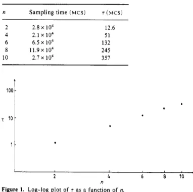
In the present work, the relaxation times for the square lattices of sizes n = 2,4,6,8, 10 were obtained for the two-dimensional Ising model with a non-conserved order para- meter. Since the sampling time is much larger than the associated time constants, we expect that the statistical errors in the time constants are very small. It should be pointed out that the main source of errors in our results is not statistical, but arise due to the relatively small values of n considered. Table 1 shows the relaxation time values
obtained from the M C simulation.
The log-log plot of T as a function of n is given in figure 1. The critical exponent z
is obtained from the slope of this graph. Its value was estimated to be z = 2.1 1, which is consistent with the range of values reported in the literature (for a recent review see Binder and Landau 1989, and Landau er a1 1988).
Table 1. Relaxation time values obtained from the MC simulation for the two-dimensional Ising model. The first column gives the sizes of the lattices. Sampling time corresponds to the number of M C S (per site) in which statistical values are taken. The last column shows the relaxation time values for these sizes.
n Sampling time ( M C S ) 7 ( M C S ) 2 2.8 x 10⁴ 12.6 4 2.1 x io4 51 6 6.5 x io4 132 8 1 1 . 9 ~ io4 245 10 2.7 x io4 351
~-
2 4 6 8 lo nRelaxation time constant of spin systems 4523 It is to be emphasized again that our method for determining the relaxation time constant is much more efficient and straightforward than extracting a time constant from time plots of spin-spin correlation.
Acknowledgment
The authors would like to acknowledge the support of the Middle East Technical University Computer Center.
References
Aydin M and Yalabik M C 1984 J. Phys. A: Math. Gen. 17 2531
Binder K 1976 Phase Transitions and Critical Phenomena vol 5B, ed C Domb and M S Green (New York: Binder K and Landau D P 1989 Advances in Chemical Physics ed K P Lawley (New York: Wiley) Hohenberg P C and Halperin B I 1977 Rev. Mod. Phys. 49 435
Kawasaki K 1972 Phase Transirions and Critical Phenomena vol 2, ed C Domb and M S Green (New York: Landau D P, Tang S and Wansleben S 1988 J. Physique C 8 1525
Metropolis N, Rosenbluth A W, Rosenbluth M N , Teller A H and Teller E 1953 J. Chem. Phys. 21 1087 Suzuki M 1977 B o g . Theor. Phys. 58 1142
Tobochnik J and Jayaprakash C 1981 Phys. Rev. B 25 4893 Academic)