Performance analysis of concatenated coding schemes

1 w -ύ 4 <ütoF А / vi:,' , , v i^ J u 4 " 4 l j „•w'*'4 J4» ü 'ϋ ύ ' J ..V W W * ,4 U '4>*Χ -Ιί ?J J ! » :J U '¿í^<ií3

PERFORMANCE ANALYSIS OF CONCATENATED

CODING SCHEMES

A THESIS

SUBMITTED TO THE DEPARTMENT OF ELECTRICAL AND ELECTRONICS ENGINEERING

AND THE INSTITUTE OF ENGINEERING AND SCIENCES OF BILKENT UNIVERSITY

IN PARTIAL FULFILLMENT OF THE REQUIREMENTS FOR THE DEGREE OF

MASTER OF SCIENCE

Gurt ALIi-Or*

By

Gün Akkor

τ κ

5·<οα .5

-АЪЪ

ІЭЭЭ

Д048793

11

I certify that I have read this thesis and that in my opinion it is fully adequate, in scope and in quality, as a thesis for the degree of Master of Science.

- = ^ Q ) k L - ^

Prof. Dr. Erdal Arikan (Supervisor)

I certify that I have read this thesis and that in my opinion it is fully adequate, in scope and in quality, as a thesis for the degree of Master of Science.

Assoc. ProL Dr. Melek Yücel

I certify that I have read this thesis and that in my opinion it is fully adequate, in scope and in quality, as a thesis for the degree of Master of Science.

3İSK Prof./Dr. M

Assist(^Prof./t)r. Murat Alanyali

Approved for the Institute of Engineering and Sciences:

Prof. Dr. Mehinet^tiaray

ABSTRACT

PERFORMANCE ANALYSIS OF CONCATENATED

CODING SCHEMES

Gün Akkor

M.S. in Electrical and Electronics Engineering

Supervisor: Prof. Dr. Erdal Arikan

June 1999

In this thesis we concentrate on finding tight upperbounds on the output error rate of concatenated coding systems with binary convolutional inner codes and Reed-Solomon outer codes. Performance of such a system can be estimated by first calculating the error rate of the inner code and then by evaluating the outer code performance. Two new methods are proposed to improve the classical union bound on convolutional codes. The methods provide better error estimates in the low signal-to-noise ratio (SNR) region where the union bound increases abruptly. An ideally-interleaved system performance is evaluated based on the convolutional code bit error rate estimates. Results show that having better estimates for the inner code performance improves the estimates on the overall system performance. For the analysis of a non-interleaved system, a new model based on a Markov Chain representation of the system is proposed. For this purpose, distribution of errors between the inner and outer decoding stages is obtained through simulation. Markov Chain parameters are determined from the error distri­ bution and output error rate is obtained by analyzing the behavior of the model. The model estimates the actual behavior over a considerable SNR range. Extensive computer simulations are run to evaluate the accuracy of these methods.

Keywords: concatenated coding, performance analysis, union bound, non-interleaved

systems.

ÖZET

Gün Akkor

Elektrik ve Elektronik Mühendisliği Bölümü Yüksek Lisans

Tez Yöneticisi: Prof. Dr. Erdal Arıkan

Haziran 1999

Bu tezde konvolusyonel iç kodlama ve Reed-Solomon dış kodlama kullanan kademeli kodlama şekillerinin sistem çıkışındaki hata olasılıkları için üst sınır bulunması üzerinde durulmuştur. Bu tür sistemlerin performansı iç kodun hata olasılığının hesaplanması ve bunun dış kodun performansının hesaplanmasında kullanılması yolu ile tahmin edilebilir. Konvolusyonel kodların hata olasılıkları üzerindeki klasik üst sınırların iyileştirilmesi için iki yeni yöntem önerilmiştir. Bu yöntemler özellikle düşük sinyal-gürültü oran­ larında hata olasılıklarını daha iyi tahmin etmektedir. Konvolusyonel kodların hata olasılık tahminleri kullanılarak bloklar arasındaki sembollerin ideal olarak düzenlendiği (interleaved) kademeli kodlama sisteminin performansı incelenmiştir. Sonuçlar iç kod­ lama hata olasılığı üzerinde elde edilen daha iyi tahminlerin, tüm sistemin hata olasılığı üzerindeki tahminleri de iyileştirdiğini göstermiştir. Bloklar arasındaki sembollerin düzen­ lenmediği (non-interleaved) kademeli kodlama sistemlerinin performansının incelenmesi için bir Markov Chain modeli önerilmiştir. Simülasyon yolu ile iç ve dış kodlama blokları arasındaki hata dağılımı elde edilmiştir. Bu dağılımdan yararlanılarak Markov modelinin parametreleri elde edilmiştir. Sistem çıkışındaki hata olasılıkları modelin davranışları in­ celenerek elde edilmiştir. Model, geniş bir sinyal-gürültü oranı için sistem performansını doğru tahmin etmektedir. Metodlarm doğruluğunun kıyaslanması için tüm incelenen sistemlerin hata olasılıkları simülasyon yolu ile de elde edilmiştir.

Anahtar Kelimeler: kademeli kodlama, performans analizi, hata olasılıkları için üst

sınırlar.

ACKNOWLEDGMENTS

I would like to express my deep gratitude to my supervisor Prof. Dr. Erdal Arikan for his guidance, suggestions and valuable encouragement throughout the development of this thesis.

I would like to thank Assoc. Prof. Dr. Melek Yücel and Assist. Prof. Dr. Murat Alanyah for reading and commenting on this thesis and for the honor they gave me by presiding the jury.

I am also grateful to my friends, Arçm Bozkurt, Ayhan Bozkurt, Deniz Gürkan, Tolga Kaxtaloglu, and Güçlü Köprülü, who made life at Bilkent more enjoyable during the course of this thesis work. I would like to thank everyone who in one way or the other helped me to complete my thesis.

Sincere thanks to Assoc. Prof. Dr. Ir§adi Aksun, for our friendly conversations and his motivation during the very last moments of this thesis work.

Duygu deserves the right to be mentioned separately for sharing all my time with me. Thank you for your encouragement, support, and understanding but above all for being with me.

My gratitude is far less than they deserve for my wonderful parents. W ithout their love, endless support, and understanding nothing would be possible.

C ontents

1 Introduction 1

1.1 Fundamental Concepts of Concatenated C o d in g ... 2

1.2 Problem S ta te m e n t... ! ... 5

1.3 Outline of the Work D o n e ... 6

1.4 Organization of the T h e s is ... 7

2 Survey of Results on Convolutional Code Performance 8 2.1 Binary Rate-1/2 Convolutional C o d es... 8

2.2 Weight Distribution of Convolutional C o d e s ... 11

2.3 Union Bound on Probability of Decoding Error 13 2.4 Other Bounds on Probability of Error of Convolutional C o d e s ... 16

3 Improved Bounds on Convolutional Code Performance 22 3.1 Improving Union Bound using Weight Distributions ... 23

3.2 Results and Discussions 28 3.3 Improving Union Bound by P a r titio n in g ... 33

v i l

3.4 Results and Discussions 35

4 Ideally Interleaved System Performance 38

4.1 Overview of Reed-Solomon C o d e s ... 38 4.1.1 Error Probability Calculation on Reed-Solomon C o d e s ... 40 4.2 Results on Ideally Interleaved S y ste m ... 41

5 Non-Inter leaved System Performance 45

List o f Figures

1.1 A communication system exam ple... 2

1.2 Concatenated coding s y s te m ... 4

1.3 An Interleaved S y s te m ... 5

2.1 Encoder for a i 2 = l / 2 , Ar = 3 convolutional c o d e ... 9

2.2 State diagram for the i 2 = l / 2 , u = 2 convolutional c o d e ... 9

2.3 Trellis diagram for the R = 1/2, K = Z convolutional c o d e ... 10

2.4 State and signal flow diagrams for the R = 1/ 2, K = 3 convolutional code 12 2.5 Some trellis p a t h s ... 15

2.6 Some error events at jth trellis s t a g e ... 16

2.7 Barrier at Vk which separates paths with many and few e r r o r s ... 19

3.1 Paths forming the set S'e, for j = 6 ... 25

3.2 State diagram for rate-1/2 constraint-length-3 c o d e ... 26

3.3 Probability of bit error for i? = 1/2, AT = 3 code over BSC with BPSK modulation ... 29

3.4 Difference that would result in calculations for L^ax = 3 5 ... 30

3.5 Probability of bit error f o r j R = l / 2 , AT = 3 code over AWGN channel with BPSK m odulation... 31

IX

3.6 Difference that would result in calculations for L^ax = 3 5 ... 32

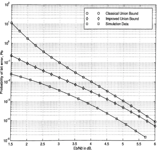
3.7 Probability of bit error for R = 1/ 2, K — 3 code over BSC with BPSK modulation ... 36

3.8 Probability of bit error for iZ = 1/ 2, K = 3 code over an AWGN channel 37 4.1 Bit error probability of ideally interleaved concatenated system over AWGN channel with soft decision ... 43

4.2 Bit error probability of ideally interleaved concatenated system over BSG with hard decision 44 5.1 An example burst and wait s tr u c tu r e ... 46

5.2 Burst and wait histograms for Ei,/Nq = 1.2dB... 47

5.3 Burst and wait histograms for Ei/Nq = 2.3dB... 48

5.4 Markov Chain representation of symbol e r r o r s ... 49

5.5 Word and symbol error probabilities for non-interleaved concatenated sys­ tem over AWGN channel and soft d e c is io n ... 52

5.6 Word and symbol error probabilities for non-interleaved concatenated sys­ tem over BSC and hard decision d e c o d in g ... 55

List o f Tables

3.1 Codewords and their distances from the all-zero codeword 25 4.1 Bit error rates at the RS decoder input for AWGN channel and soft deci­

sion d e c o d in g ... 42 4.2 Bit error rates at the RS decoder input for BSC channel and hard decision

d eco d in g ... 42 5.1 Mean burst and wait lengths in symbols for AWGN channel with soft

decision d e c o d in g ... 50 5.2 Calculated word and symbol error probabilities at the system output for

AWGN channel case ... 51 5.3 Simulation data for the word and symbol error probabilities at the system

o u t p u t ... 51 5.4 Mean burst and wait lengths in symbols for BSC with hard decision decoding 53 5.5 Calculated word and symbol error probabilities at the system output for

BSC case ... 53 5.6 Simulation data for word and symbol error probabilities at the system

G lossary

A W G N : Additive White Gaussian Noise

B D D : Bounded Distance Decoder

B E R : Bit Error Rate

B S C : Binary Symmetric Channel

B P S K : Binary Phase Shift Keying M C : Markov Chain

M L : Maximum-likelihood

R S : Reed-Solomon

S N R : Signal-to-noise Ratio d : Hamming distance

k : Number of information symbols in a codeword

K : Constraint length

m : Number of bits in a RS symbol

n : Codeword length

Pb : Probability of bit error

Pc : Probability of correct decoding P e : Error event probability

Pe : First error event probability

Ps : Probability of symbol error

Pw : Probability of word error R : Rate of a code

T (D ) : Path enumerator of a convolutional code t : Number of correctible RS symbol errors V : Memory of a convolutional code

Chapter 1

Introduction

Error control coding is an area of increasing importance in communication. This is partly because the data integrity is becoming increasingly important. There is downward pressure on the allowable error rates for communications and mass storage systems as bandwidths and volumes of data increase. In any system which handles large amount of data, uncorrected or undetected errors can degrade performance.

Just as important as the data integrity issue is the increasing realization that error control coding is a system design technique that can fundamentally change the trade-offs in a communications system design. Even if a communications system has no problem with the data quality, designers may consider discarding or downgrading the most expen­ sive or troublesome elements while using the error control coding techniques to overcome the resulting loss in performance.

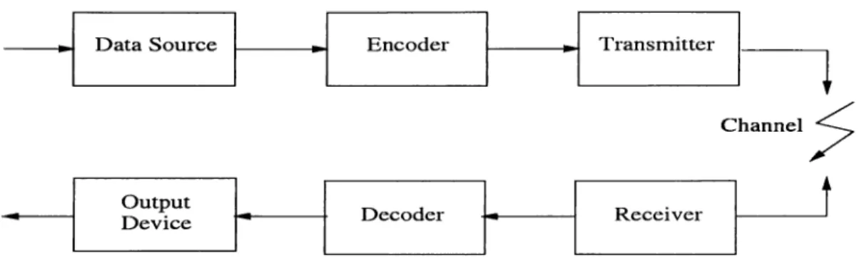
An oversimplified structure of a communications system is shown in Fig. 1.1. Data symbols generated by the source are encoded and then transmitted through the channel. Due to presence of noise, some of the symbols are received in error at the other end. Decoder processes the received data in an attem pt to minimize the number of symbols in error. A natural measure of data integrity at the system output is the probability of

symbol error, F«, which is the ratio of symbols in error to the overall number of trans­

mitted symbols. Performance of a coding scheme can be evaluated based on the error rate at the output when all other system parameters (channel properties, transmitter power, etc.) are kept constant.

C h a n n e l

Figure 1.1: A communication system example

In system design, an estimate on the performance of a particular coding scheme is essential to decide on the system parameters. The most useful techniques for estimating the performance of a code are computer simulations and error bounds. The usefulness of computer simulation is limited by the long computational times that are required to get a good statistical sample (it may take several hours to get a single point). Bounds on the error performance, on the other hand, aim to find analytical models to the actual behavior. They require less computational effort, but may not be able to predict the behavior of the code over the full operation range, or may overestimate the actual error rate.

Problem of finding tight bounds on the error rate of different coding schemes is an active research area. The problem of interest in this thesis is to find tight bounds on the error performance of concatenated coding schemes. Most of today’s system appli­ cations require low rates of error. This can be accomplished by imposing codes with longer block lengths and larger error-correcting capabilities. However, encoder/decoder complexity also increases placing a burden on implementation. In concatenated coding, this problem is overcame by utilizing multiple levels of coding where each stage has mod­ erate complexity. In the next section, fundamental concepts of concatenated coding is discussed.

1.1 Fundamental Concepts of Concatenated Coding

When digital data are transmitted over a noisy channel, there is always a chance that the received data will contain errors. The user generally establishes an error rate below which the received data are usable. If the received data will not meet the error rate

requirement, error-correction can often be used to reduce errors to a level at which they can be tolerated. In recent years the use of error-correction coding for solving this type of problem has become widespread.

The utility of coding was first demonstrated by the appearance of Shannon’s classic paper [1]. In 1948 he proved that as long as the data source rate is less than the

channel capacity, communication over a noise channel with an error probability as small

as desired is possible with proper encoding and decoding. Essentially, Shannon’s work states that the signal power, channel noise, and available bandwidth set a limit only on the communication rate and not on the accuracy.

It soon became clear that the real limit on communication rate was set not by the channel capacity but by the cost of implementation of coding schemes. Cost constraints force communication at rates substantially below capacity. In recent years much research has been directed toward finding efficient and practical coding schemes for various types of noisy channel. Concatenated coding, which was first investigated by Forney [2], is a way of achieving low error probabilities using long block length (linear) codes at rates below capacity without requiring an impossibly complex decoder.

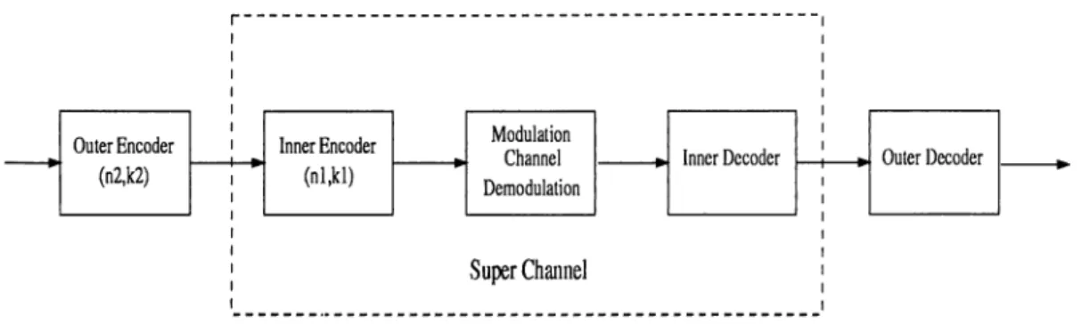
The basic idea behind concatenated coding is that the “encoder-channel-decoder” of a normal communication system can be viewed as a kind of superchannel for which an outer code can be employed (Figure 1.2). If length, dimension, and minimum Hamming distance for the inner and outer (block) codes are denoted by (ni, k i,d i) and (ri2, k2, ¿2), respectively, it is then well known that the corresponding concatenated code has length

n = niri2, dimension k = k ik 2, and minimum Hamming distance d > d\d2 with equality

if every nonzero codeword in the inner code has constant weight. Concatenation is then a technique for producing long codes from short codes. This property is particularly important for the receiver-side operation. Though shorter codes have weaker error cor­ rection capabilities, they have simpler decoding mechanisms. Inner decoding and outer decoding are performed separately on the receiver side allowing the overall decoding complexity to remain moderate. On the other hand, decoding errors made by the inner decoder can be corrected by the outer decoder improving the overall performance.

Though numerous configurations are possible, concatenated coding systems with Reed-Solomon (RS) outer codes and binary convolutional inner codes are popular. Bi­ nary convolutional codes work on binary (0 or 1) digits or bits. The encoder of such codes maps a binaxy input sequence into a binary output sequence. Binary convolutional codes are particularly effective in correcting uniformly distributed bit errors. However, closely

Figure 1.2: Concatenated coding system

spaced bit errors are decoded into an error burst due to presence of decoder memory. A detailed discussion on convolutional codes is presented in Chapter 2.

RS codes work on a higher alphabet of m-bit symbols. They map every k information symbols into a codeword of n = 2"^—1 symbols. Such a code can correct any t = {n—k )/2 symbol errors in a n symbol codeword. Considering a bounded-distance-decoder (BDD) which corrects all error patterns of weight t or less and corrects no patterns of weight larger than t, probability of correct decoding for a (n, k) RS code is given by

(

.

)

In cases where burst errors are a problem, one potential solution involves the utiliza­ tion of a suitable interleaver/deinterleaver pair between the inner and outer stages. Using this approach, output sequence of outer encoder is interleaved prior to inner encoder at the transmitter side. The output sequence of the inner decoder is then deinterleaved prior to outer decoder at the receiver side. A system block diagram is shown in Fig. 1.3. An interleaver is a device th at rearranges (or permutes) the ordering of a sequence of symbols in a deterministic manner. Associated with an interleaver is a deinterleaver that applies the inverse permutation to restore the sequence to its original ordering. When deinterleaving is applied on the receiver side, the burst errors caused by the inner

Outer _Interleaver Super _{Deinterleaver} Outer

Encoder Channel Decoder

Figure 1.3: An Interleaved System

decoding are distributed more uniformly prior to outer decoder increasing the overall probability of correct decoding.

Concatenated schemes are one of the most effective coding systems. In the next section, we state two basic problems of performance analysis of concatenated systems.

1.2 Problem Statement

In this thesis, we restrict our attention to two-stage concatenated schemes with rate-1/2 binary convolutional inner codes, and RS outer codes. The performance of such a system based on a probability of symbol error measure can be calculated by first estimating the symbol error rate of the inner convolutional code and then by evaluating the error rate of the outer RS code. The probability of symbol error for a convolutional code can be upper bounded by using the well-known union bound and path enumeration techniques. This bound matches exact behavior at high signal-to-noise ratio (SNR) region, but is rather loose as we move to the low SNR region. This region is the target operational range for concatenated schemes. Therefore, if classical union bound is used to evaluate the inner code performance, the resulting bound will be loose in the range of interest. For a better estimate on the overall system performance, the classical union bound should be modified in the low SNR region.

There exists closed form expressions for calculating the probability of error at the RS decoder output based on the probability of error estimates at the input. But such expressions assume that the symbol errors at the decoder input are independent of each other. For the inner decoder operation this might be validated under the assumption that the channel is memoryless. However, convolutional codes have memory, and a single error appearing at the decoder input may propagate and form a burst of errors at the output. Consequently, the symbol errors at the RS decoder input are not independent of each other. The same expressions can be used under the assumption that interleaving/de­ interleaving is applied between the stages. However, for non-interleaved cases, a model

that takes the bursty nature of errors into account should be devised.

1.3 Outline of the Work Done

In an attem pt to improve the union bound on convolutional codes, we generalized the results of [3] for convolutional codes. In [3] an improved union bound for the binary input AWGN channel in terms of the weights of the codewords of a linear block code is presented. For the convolutional code case, we treated every path that diverges from the all-zero path at the origin and merges back at the jth trellis stage as a codeword of length rij = 2j for a rate-1/2 code. Paths of length Uj form a set, Sj, of codewords of equal length. The process of partitioning paths into codewords of equal length can go up to infinity, with increasing j. However, the probability that a path will stay diverged from the all-zero path for a large j decreases. Therefore, we limit j to be less than or equal to some constant Lj^ax- Every set Sj is then treated as a block code of blocklength Uj for which the arguments of [3] can be applied. The overall probability figure is obtained by summing the individual results. This method is applied to both a binary symmetric channel (BSC) with hard decision decoding and an AWGN channel with soft decision decoding. The method provides promising results. The results show 2 to 10 fold improvement over the classical union bound.

The second approach to improve the union bound on convolutional codes calculates the probability of error as a sum of two terms. If a sequence of weight less than i is received, then we use the path enumerator polynomial to calculate the probability of error of this case. A sequence of weight less than i can be decoded into any path of weight df < d < 2{i — 1) by a maximum-likelihood (ML) decoder, where df is the free distance of the convolutional code. Therefore, only these terms of the path enumerator polynomial is used in the summation. If a sequence of weight larger than i is received, we assume that the decoder always makes an error and hence in this case the probability of error is equated to the probability of receiving such a path. The overall probability of error is given by the sum of the two cases. The value of i changes the contribution of the two cases. Therefore, we repeat the calculations for i running from \ d f / 2], which is the minimum number of channel errors that may cause the received sequence to be decoded into a wrong path, to [dma®/2] which is the number of channel errors that may cause the received sequence to be decoded into a path that is most far away from the

correct path assuming that we use a truncated code. Then, the minimum is chosen as the error probability. This approach provides improvement in the low SNR region. In the high SNR region the bound tends to converge to the classical union bound.

To deal with the non-interleaved cases, we run extensive computer simulations to obtain burst histograms for the convolutional code. Also, histograms for the distribution of waiting times between the occurrence of successive bursts are obtained. The results are used to set up a two state Markov Chain model; the states representing the events of a symbol being correct or erroneous. The steady state distribution of the Markov Chain is then used to calculate the probability of symbol error for the outer RS code. The model provides almost exact results over a considerable range of SNR values. At high SNR region, the results show deviation from the exact behavior as the assumption of geometrically distributed waiting times does not correctly model the system.

Finally, computer simulations are run for both a BSC with hard decision decoding and an AWGN channel with soft decision decoding. These data are used to evaluate the accuracy of the above methods. The details of all methods and their results are extensively discussed in Chapter 3 and Chapter 5.

1.4 Organization of the Thesis

The organization of the thesis is as follows. In the next chapter, following an overview of convolutional codes, a survey of results on convolutional code performance is presented. Chapter 3 includes a detailed discussion on the work done to improve the union bound at low SNR region and presents the results. In Chapter 4 RS code structure and its properties are presented and an ideally interleaved system performance is evaluated based on the results of Chapter 3. In Chapter 5 work done to model the bursty behavior of symbol errors at the RS decoder input is presented. Based on these results a non- interleaved system is investigated. In the final chapter an overall conclusion is presented and possible future work is discussed.

Chapter 2

Survey o f R esults on C onvolutional

Code Perform ance

In this chapter, an overview of convolutional code structure is presented. Following a discussion on weight distribution of convolutional codes, the classical union bound on probability of error is introduced. Finally, a survey of results on convolutional code performance is presented.

2.1 Binary Rate-1/2 Convolutional Codes

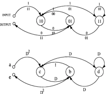
A constraint length K convolutional encoder consists of a K-st&gQ shift register with the outputs of selected stages being added modulo-2 to form the encoded symbols. A simple example is the i? = 1/2 convolutional encoder shown in Fig. 2.1. Information symbols are shifted in at the left, and for each information symbol the outputs of the modulo-2 adders provide two channel symbols. The connections between the shift register stages and the modulo-2 adders are conveniently described by generator polynomials. The polynomials g\{D) = 1 + D + and g^iD) = 1 -f- represent the upper and lower connections, respectively (the lowest-order coefficients represent the connections to the leftmost stages). The input information sequence can also be represented as a power

series I{D ) = ¿0 + i^D + ¿2-0 ^ + ..., where ij is the information symbol (0 or 1) at the jth symbol time. With this representation the outputs of the convolutional encoder can be described as a polynomial multiplication of the input sequence, I{D ), and the code generators. For example, the output of the upper encoded channel sequence of Fig. 2.1 can then be expressed as Ti{D) = I{D)gi{D), where the polynomial multiplication is carried out in G F (2).

1(D ) I N P U T

Figure 2.1; Encoder for a = 1/2, /(T = 3 convolutional code

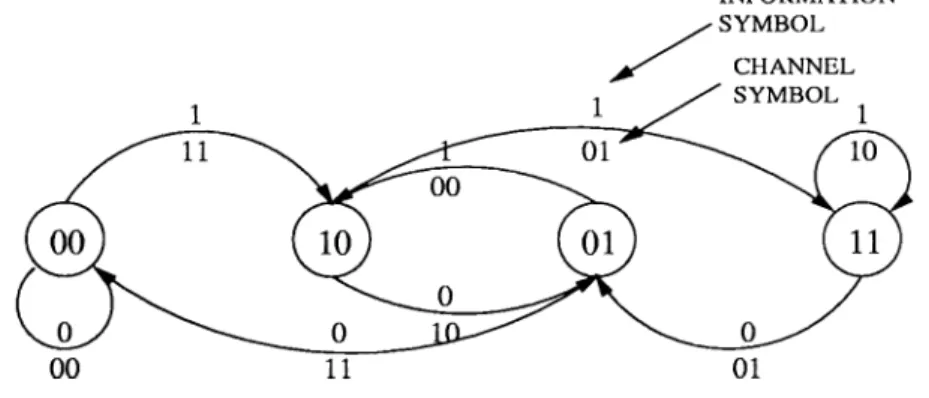
It is possible to view the above convolutional encoder structure as a finite-state machine. The state of a convolutional encoder is determined by the most recent v = K —1 information symbols shifted into the encoder shift register. The state is assigned a number from 0 to 2*' — 1. The current state and the output of the encoder are always uniquely determined by the previous state and current input. A complete description of the encoder as far as the input and the resulting output are concerned can be obtained from a state diagram, as shown in Fig. 2.2 for the R = 1/ 2, v = 2 {K = 3) code. The symbol along the top of the transition line indicates the information symbol at

INFORMATION

Figure 2.2: State diagram for the R = 1/ 2, v = 2 convolutional code

10

show the resulting channel symbols at the encoder output. Any sequence of information symbols dictates a path through the state diagram, and the channel symbols encountered along this path constitute the resulting encoded channel sequence.

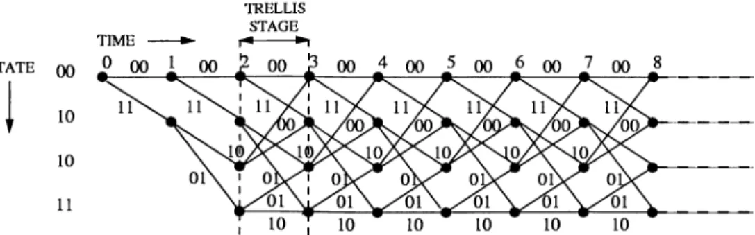
Because of the topological equivalence between the state diagram of Fig. 2.2 and a signal flow graph [4], the properties and theory of signal flow graphs have been applied to the study of convolutional code structure and performance. The state diagram of a convolutional code can be alternatively viewed as in Fig. 2.3. This structure has been given the name trellis structure, and has proved to be useful in performance analysis as well as in the study of decoding algorithms.

TRELLIS STAGE TIME

Figure 2.3: Trellis diagram for the i? = 1/ 2, AT = 3 convolutional code

Decoding of convolutional codes can be accomplished by a maximum-likelihood de­ coding algorithm known as Viterbi algorithm [5]. The Viterbi algorithm operates step by step, tracing through a trellis identical to that used by the encoder in an attempt to emulate the encoder’s behavior. At any time the decoder does not know which node the encoder reached and thus does not try to decode this node yet. Instead, given the received sequence, the decoder determines the distance between each such path and the received sequence. This distance is called the discrepancy of the path. If all paths in the set of most likely paths begin in the same way, the decoder knows how the decoder began.

Then in the next trellis stage , the decoder determines the most likely path to each of the new nodes of that stage. But to get to any of the new nodes the path must pass through one of the old nodes. One can get the candidate paths to a new node by extending to this new node each of the old paths that can be thus extended. The most likely path is found by adding the incremental discrepancy of each path extension to the discrepancy of the path to the old node. There are 2" such paths to each node, and the path with the smallest discrepancy is the most likely path to the new node. This process

11

is repeated for each of the new nodes. At the end of the iteration, the decoder knows the most likely path to the each of the nodes in the new trellis stage.

Consider the set of surviving paths to the set of nodes at the jith trellis stage. One or more of the nodes of the first stage will be crossed by these paths. If all the paths cross through the same node at the first trellis stage, then regardless of which node the encoder visits at the jth stage, decoder knows the most likely node it visited at the first stage. That is, the first information is known even though no decision can be made for the j th stage. To build a Viterbi decoder, one must choose a decoding-window width

W , usually several times as the constraint-length. At jth stage, the decoder examines

all surviving paths to see if they agree in the first branch. This branch defines a decoded information frame, which is passed out of the decoder. Next the decoder drops the first branch and takes a new frame of the received word for the next iteration. If again all surviving paths pass through the same node of the oldest surviving trellis stage, then this information frame is decoded.

The process continues in this way, decoding frames indefinitely. If W is chosen long enough, then a well-defined decision will almost always be made at each stage. In some cases, the surviving paths might not all go through a common node, or may converge into a wrong node. In such cases a decoder failure or a decoding error occurs. If the errors occur randomly, with enough spacing in between, the decoding algorithm chooses the correct path with high probability. However, if errors occur in bursts, decoder algorithm may fail to decode to the correct path causing an error burst at the output.

The Viterbi algorithm and the trellis structure provides a framework for the calcula­ tion of weight distributions and performance bounds using path enumeration techniques.

2.2 Weight Distribution of Convolutional Codes

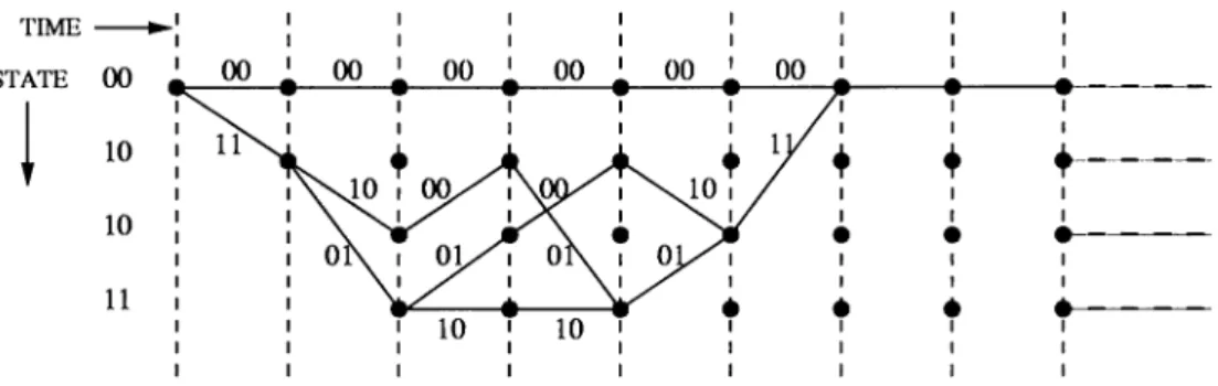
Weight distribution of a code has particular importance for evaluating the performance of the code. Calculation of the weight distribution of convolutional codes requires the examination of the state diagram structure of Section 2.1. The weight of a convolutional codeword, infinitely long, is the number of nonzero components it has. If the code is simple enough for the trellis to be drawn, all of these parameters can be read from the trellis. For example, consider the R = 1/2, K = 3 convolutional code which has the

12

trellis structure shown in Fig. 2.3. Tracing the trellis it is found that there is a path of weight 5, that occupies three stages. This is also the free distance of the code. The free distance of a convolutional code is defined as the distance of the shortest path that diverges from the all-zero path at the origin and merges back at a later trellis stage. Looking further, there are two paths of weight 6, four paths of weight 7 and so on. In this way the number of paths of each weight can be enumerated, but this quickly becomes tedious. A more powerful approach uses the state diagram of the code and the theory of signal flow diagrams to determine the complete weight distribution [6].

D D

Figure 2.4; State and signal flow diagrams for the R = 1/2, K = 3 convolutional code In Fig. 2.4, the state diagram of Section 2.1 is redrawn. Note that the state labeled 00 is drawn twice, once as input and one as output, because we are only interested in paths starting at 00 and ending at 00. Also each branch is attached a gain as power of a dummy variable D. The weight of a branch now appears as the power of D. The weight of a path is obtained by multiplying all the gains along the path. It is possible to compute the gain T{D ) of the whole network between the input and the output by simultaneous solution of the following equations obtained from Fig. 2.4:

b c d e Dc + Dd Dc Dd D ' \ (2.1)

13

Solution of these equations gives

e =

1 - 2Da. (2.2)

Thus the path enumerator is

T iD ) = ---^ ’ I - 2 D

= + . . . + + . . . . (2.3)

Comparing the expression in Eq. 2.3 with the trellis diagram of Fig. 2.3 one can verify that there are actually 2* paths of weight i + 5. The same technique can be used to count other properties of the code. Introducing two new dummy variables, L to count the number of trellis stages, and I to count input ones, and solving as before,

D^L^I T ( D ,L ,I ) =

1 - D L {1 + L )I

= D^L^I + D ^ L \ l + L)I^ + + L f l ^

+ . . . + + . . . (2.4)

Thus, the path of weight 5 has a length of 3 and is caused by a single input bit equal to one. There are two paths of weight 6, each caused by two input ones; one path has length 5 and one has a length of 6. In this way the distance structure which is needed for bounding the probability of error can be fully determined.

2.3 Union Bound on Probability of Decoding Error

This technique can be used for any block or convolutional code with maximum-likelihood decoding. It is based on the following idea. If an event can be expressed as the union of several subevents, then the probability of that event is less than or equal to the sum of the probabilities of all subevents.

n-l

P(A) = P(A^

U ■

· ■

U ^ -i) ^ E

¿=0

(2.5) This sum is obviously an over-bound since it counts the contribution due to overlapping events more than once.

14

In the case of a linear block code, the probability of error can be computed by considering the effect of transmitting the all-zero codeword. An error will be made if the received sequence (the term ‘sequence’ is introduced here because in general a received sequence may not be equal to any of the valid codewords due to errors) is closer to one of the other codewords than it is to the all-zero word. Thus, the probability of error can be over-bounded as the sum of the probabilities of each of these individual error events. Define Aq as the event of transmitting the all-zero codeword and Bj as the event

that distance between the received sequence and some codeword of weight j is smaller than the distance between the received sequence and the all-zero codeword. Using this approach the probability of codeword error for a maximum-likelihood decoder is upper bounded by [7]

P y : < f 2 ^jP(Bj/Ao), (2.6) i=l

where Cj is the number of codewords of weight j. In a similar fashion the average bit error probability is upper bounded by

a < E f c j P i B j / A o ) ,

j=i

(2.7) where r]oj is the average number of nonzero information bits associated with a codeword of weight j and k is the number of information bits in a n bit codeword. The term rjoj/k can be very closely approximated hy j / n [7]. P(Bj/Ao) for the case of a BSC with hard decision and cross-over probability of p, is given by

f

p , = p ( B , M o ) = ^ . . . (2.8) Eq. 2.8 can be upper-bounded by the Chernoff bound [8]

P, < [2\/p(l - p)]’ (2.9) For an AWGN channel, a similar expression can be given as below assuming white Gaussian noise with (two-sided) power spectral density Nq/2 and an energy of y/E l per

symbol with BPSK modulation [9].

Pi = P (Bi/A o) = j e r f c ( ^ ) (2.10) Eq. 2.10 can be approximated as [6]

(2.11)

_iMa.

15

Ideas presented in this section can be directly applied to the computation of error probability for binary convolutional codes. There are, however, several possible defini­ tions of error probability, and each must be handled slightly differently [10]. Without loss of generality, assume th at the all-zero path is transmitted. This means that the path followed by the encoder is the horizontal path at the top of the trellis diagram (Fig. 2.3). The decoder does not know which path the encoder has followed, but will make a guess based on the received noisy version of the transmitted path. The path actually taken by the encoder is called the correct path and the path postulated by the decoder is called the decoder’s path. The decoder’s path can clearly be partitioned into a (possibly empty) set of correct path segments separated by a set of paths which lie entirely below the correct path expect for their end points (Fig. 2.5). These incorrect path segments are called error events.

d e c o d e r ’ s p a th

Figure 2.5: Some trellis paths

The first error event probability is defined as the probability that the decoder will be off the correct path at the origin. For a maximum-likelihood decoding algorithm, such as Viterbi algorithm, this is possible if a path of weight j , that diverges from the all-zero path at the origin, is closer to the received sequence than the all-zero path. If Pj denotes the probability of this event, then

Pj < 7^' (2.12) where 7 is a channel dependent parameter (see Eq.’s 2.9 and 2.11). Using union bound, probability of first error event is bounded by

3

(2.13) where Cj is the number of paths of weight j that diverge from the all-zero path at the origin. Since Cj are given by the coefficients of the path enumerator T{D) of the convolutional code, Eq. 2.13 can be written by [11]

16

Another possible case of interest is the error event probability, Pg, which is the prob­ ability th at the decoder is off the correct path at the jth trellis stage. This is just the probability th at there is an error event hanging below the correct path at jth stage (Fig. 2.6). By a reasoning similar to the derivation of Eq. 2.14, an upperbound on the

Figure 2.6: Some error events at jth trellis stage probability of error event is given by [11]

dT{D, L, I) Pe <

dL Drr7,L= 1,7=1 (2.15)

The decoder outputs information bits corresponding to its postulated path, and that even if it is on the wrong path, some of the individual bits will be “accidentally” right. Thus the bit error probability, Pb, will in general be less than the error event probability. Using a reasoning similar to that leading to Eq. 2.7, the following bound on Pb is obtained

(111:

n < 1 (2.16)

K dl D=7,L=1,7=1

for a rate-fc/n binary convolutional code. In both cases, 7 equals either Eq. 2.9 or 2.11 depending on the channel.

2.4 Other Bounds on Probability of Error of

Convolutional Codes

The ideas presented in the previous sections have been extended to tighter bounds on the error performance of various coding schemes. As we stated earlier, the performance of a concatenated code can be evaluated by first estimating the symbol error rate of the inner code and then calculating outer code performance. Therefore, the problem of computing

17

the overall performance of a concatenated system is equivalent to finding good estimates for the inner convolutional code performance. In this respect, this section presents other research on finding improved bounds on error performance of convolutional codes.

In [12], tighter upper bounds on the error-event and bit error probabilities axe derived from Viterbi’s upper bounds for the case of a BSC with maximum-likelihood decoding. Prom Eq. 2.8, it is observed that P271 = P2n-i, n = l , 2, — Then,

P2n < '2n — V n

)—2n

(2v®2n (2.17)

Since the term in square brackets is monotonically decreasing,

^2ua — 1'' P2n < t'O Tin j 2~2no (2v^)2n = r „ ,( 2Vp)2n (2.18) for n > no > 1. Finally since P2n = p 2n-i, n = 1>2, ..., Eq.’s 2.14 and 2.16 can be rewritten as,

Pe < r „ ,( j[T (D ) + T {-D )] + \d [T(D) - r ( - 0 ) ] ) c = , ^ (2.19) n < T „ ( ^ [ T ( D , I) + T ( - D , /)] + \ d \T(D, N ) - T ( - D , M)l)s,=i,i,=2^ (2.20)

respectively, where 2no is the index of the first even nonzero coefficient in T{D). The bound is evaluated for rate-1/2 code with generators polynomials 1 + D + D"^ and 1 + D^. The comparison shows significant improvement over union bound.

Later in [13], a method for explicit evaluation of Viterbi’s union bound for a BSC with maximum-likelihood decoding is proposed. The method uses the observation that A n = A n -i, n = 1, 2, . . . . Furthermore,

An+i = P 2 n - { \ - p ) (2.21)

for n = 1, 2, 3, . . . . Combining these results, the generating function F for the sequence

Pi, P2, P3, . . . can be written as follows

18

Then, for evaluating the error-event probability, T(D) is written as a rational function of the complex variable z which has the Taylor expansion

T(z) = Y , hz" (2.23) fc=l

around z = 0. Using partial fractions, T{z) can be decomposed into a polynomial t{z) and a sum of rational terms in z depending on the distinct zeros of T(z) and their multiplicities. It is shown th at the latter term can be expressed as a sum of derivatives of F(z). Then the error-event probability is bounded by

Pe < tiPi -t- Í2-f2 + ·.. + trPr + terms o f F \ z ) (2.24) where r is the degree of t{z). The same approach is applicable to the explicit evaluation of the bit error probability if is expressed as a rational function in 2:. Comparison with experimental results shows that the method provides an improvement over results of [5] and [12].

In [14], a method based on finite Markov chains is described to calculate the error- event probability of convolutional codes with maximum-likelihood decoding. Results are presented for short constraint length convolutional codes.

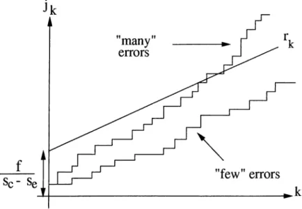
In [15], a new upper bound on error-event probability is proposed. Starting from the fact that Viterbi’s union bound is quite tight when there are few channel symbols in error (high signal-to-noise ratio) but rather loose when there are many errors, the error-event is separated into two disjoint events corresponding to few (F) and many (M) errors. Then for a BSC with maximum-likelihood decoding, probability of error-event,

P[E] is given by,

P[E] = P[E/F]P[F] + P[E/M]P[M] < P[E/F]P[F] + P[M]

= P[E, F] -f P[M] (2.25) To obtain an upper bound on P[M] a random-walk argument is used. If a metric Sg is used when a channel error occurs and a metric Sg when the channel symbol is correctly received, then the cumulative metric along the correct path is a random walk with P[zi =

Se] = p and P[zi = Sc] = {1 — p), where Zi form a sequence of statistically independent,

identically distributed random variables. If Sk denote the cumulative metric for the first

k channel symbols which have jk errors among them, then

19

Those error patterns for which Sk < —f are said to have many errors. Based on a lemma given by Gallager [8], an upper bound on P[M] is given as

P[M] = P min Sk < - f

k < 2~f (2.27)

where / is a parameter to be chosen later. Similarly, those error patterns for which

Sk > —f said to have few errors. Equivalently,

jkSe + { k - jk)sc > - / , for all k

jk < + k —^ ^ = rk, for all k

(2.28) 5c —5e

To upper bound P[E, F], first union bound is used to obtain,

k i

(2.29) where Eki is the event that a path of length k and weight i is causing an error. A path has few channel errors only if it stays below the barrier in Fig. 2.7 for all k. If all paths

Figure 2.7: Barrier at rk which separates paths with many and few errors

of length k with jk < rk channel errors are counted, all paths with few channel errors together with the paths with many channel errors that take one or more detours above the barrier will be taken. Hence,

20

where

P[Ekh3k <Tk] = Y , ^’'P[Eki/jk]·

Jk<rk

(2.31) In [15], it is shown that starting from Eq. 2.31, P[E, F] is bounded by,

, //(a c-3 e ) <PoQ' where, VP P[E,F] < '‘^T{D,I) \ P o Q / Po = < P VP + Q qo = l - p o > q (2.32) (2.33) (2.34) for 0 < 7/ < 1. The new upper bound on error-event probability is obtained by combining Eq. 2.27 and Eq. 2.32,

P[E] < \poq/

f/{Sc-3e]

T { D , I ) + 2 - f (2.35) The above bound is valid for all / . The parameter / is chosen so as to minimize the right handside of Eq. 2.35. Comparisons show that this bound is better than Viterbi’s bounds and bounds proposed in [12].

In [16], new upper and lower bounds and approximations on the sequence, event, first event, and bit-error probabilities of convolutional codes are presented. Each of these probabilities are precisely defined and the relationship between them described. Some of the new bounds are found to be very close to computer simulations at low signal-to-noise ratios. Also simple modifications to the traditional union upper bound are described for both hard- and soft-decision channels that allow better performance estimates to be made.

In [17], a Markovian technique is described to calculate the exact performance of a convolutional code with Viterbi decoding over binary symmetric channels. The Hamming distance dn between two sequences, defined as the number of bits in which they differ, is used as the decoding metric. denotes a received sequence of length N time units. Viterbi algorithm at each node 7 of the trellis diagram chooses a maximum-likelihood path among the paths leading to that node and a metric is computed from the metrics at time unit — 1. For a maximum-likelihood path A!^,

21

_jV

The relative metric, , at node 7 is obtained by subtracting the minimum metric

among all nodes from

d!; = (2.37)

The metric vector at time unit N is

(2.38) where 2" is the number of states of the convolutional encoder. These internal states of the Viterbi decoder form the Markov chain, with the received symbol r in the sequence at time N determining the transitions from one state to another. For example, the Hamming distance between a branch label and a channel output is at most two for a rate-1/ 2, 2-state convolutional code with generator matrix [1, 1-l-D]. The possible metric vectors or states of the Markov chain are therefore (2,0), (1,0), (0,0), (0,1), (0 ,2). The transition probability matrix T for the resulting Markov chain can be easily formed by checking which received signals determine a transition from one metric vector to next. The conditional probability of this received signal defines the transition probability. The probability of bit error is computed from the steady-state behavior of the Markov chain.

At a given state of the Markov chain, the exact bit error probability for the current

k information bits is computed by considering all future received sequences that stem

from a particular decoded branch. Given metric state D and a received sequence of

I branches, P { r \ D ) = i f k if z information bits are decoded incorrectly. Averaging over

all metric states and received sequences, the probability of error can be expressed as n = E W i ’('-'.D)

D ,r‘

(2.39) where qj.i is the probability of receiving sequence r* and is the steady-state distribu­ tion of the metric state D. It is understood that the received sequences in Eq. 2.39 are mutually disjoint and exhaust all possibilities that cause errors in the current time limit. The main problem encountered in calculating Eq. 2.39 is cataloging all possible future received sequences that cause information bits in a given time unit to be decoded incor­ rectly. In [17], three different approaches are introduced to overcome this difficulty. This method has limitations due to the rapid increase in the number of Markov states as the constraint length increases. These problems are addressed in [17]. For short constraint length codes, calculations are compared to simulations which show acceptable accuracy.

Chapter 3

Im proved Bounds on Convolutional

Code Perform ance

Estimating the error performance of a concatenated coding scheme requires the evalua­ tion of the error performance of the inner code. Union bound for convolutional codes, in its classical form given by Viterbi [11], is a well known approach to estimate the error performance, provided that the bit error rate (BER) at the ML decoder output is very low, for example, around 10'^ (for constraint lengths up to seven) or 10“® (for constraint lengths greater than seven). When convolutional codes are used as inner codes in con­ catenated systems, however, the codes should be optimized for a BER of around 10“^ to 10“® (the outer code takes this error rate and produces an output error rate of 10“® to 10“ ^°) [16]. Unfortunately, the accuracy of the union bound is limited in this latter range of operation (low SNR).

In this chapter, we propose two different methods for improving the union bound for binary convolutional codes. The first method is based on the ideas presented in [3] for linear block codes over a binary input AWGN channel. The results of [3] are extended to the convolutional codes over a BSC with hard decision decoding and an AWGN channel with soft decision decoding. In Section 3.1, this approach will be presented using a rate-1/ 2, constraint-length-3 convolutional code with the generator matrix g{D) =

[1 + D D " ^ ] . Results will be compared to classical union bound and to simulation

data.

23

The second method aims to improve the union bound in the low SNR region. In Section 3.3, a detailed analysis of this approach will be presented using the same exam­ ple code. Results will be presented and be compared to classical union bound and to simulation data.

3.1 Improving Union Bound using Weight

Distributions

We will first consider a linear block code of length n symbols over a binary input sym­ metric channel with BPSK modulation and following properties :

1. A binary input alphabet X = {0, 1}.

2. An output alphabet Y taking either continuous values with conditional probabil­ ity density function Px{y) or discrete values with conditional probability Px{y), depending on the channel.

3. The symmetry condition Po{y) = P i ( - y ) or po{y) = Pi{—y) holds for all outputs

y-For such a code, all non-zero codewords can be grouped according to their weights d (or distance from the all-zero codeword) into subsets xa for dmin < d <

dmax-Then for a decoder which determines the most likely codeword according to some (optimum) metric on the received vector y, the word error probability given all-zero codeword xq was sent is equal to

d=dmax

Peo = P[ U ( 3.ny codeword in has metric > that of Xp )]

d=dmin

d~dmax

< P ( any codeword in Xd has metric > that of ^ )

d=dfnifi

d=dmax

= E Pm(d)

d—dmin

In [3], based on a result of [18], it is shown that

Pm{d) < exp[-nE{5)]

(3.1)

24

where

= max{-p[r(i) + iln/i(p) + (l-i)ln.9(p)]

- ( 1 - p) ln[h(p) + p(p)]} (3.3) Here δ = d/n, r{5) = (In AT^/n), and = Size of Subset χ^, and

poo Kp) = f (3.4) Joo poo y{p) = / \ P o { y Y ^ ^ ^ ^ " ^ (3.5) Joo

for the continuous output case, and

h(p) = + (3.6)

y

M = E I a ( y ) ‘' “ +‘’> + i'o (-!/)‘^“ +'’>]-'‘- ‘’>/’o(!/)"/<'+''> (3.7) for the discrete output case. Eq. 3.1 results in a tighter union bound for linear block codes in terms of the weights of the codewords. Letting p = 1 in Eq. 3.3 results in the traditional union bound. Usually, the bit error probability is a more interesting measure on the performance. An upper bound on the bit error probability can be obtained, following the results of Section 2.3 and using Eq. 3.1, as

d—dmax

n< Σ -ί’Εθ('ί)

d=drr n

(3.8) This method can be modified for use with convolutional codes. An apparent problem is that convolutional codes have infinite length sequences or paths as codewords. To overcome this difficulty, first consider the path rji, which is the zth path that diverges from the all-zero path at the origin and merges back at the j th trellis stage. Such a path has length Uj = 2j bits for a rate-1/2 binary convolutional code. Let the distance of this path from the all-zero path be dji. We form a set Sj defined as

Sj = {paths rji of length Uj for i = 1, 2, . . . , M — 1

and the all-zero path, rjo, of length Uj} (3.9) where M is the total number of such paths. An example of such paths is shown in Fig. 3.1 for the case of rate-1/2, constraint-length-3 code with generator matrix [1 -f

25

Figure 3.1: Paths forming the set 5'e, for j = 6

Uj with M codewords. The elements of the set Sq of Fig. 3.1 and their distances from the all-zero codeword are listed in Table 3.1. Note that the set contains two codewords of distance 7 and one codeword of distance 8. Then, the codewords in a set Sj can be further grouped into subsets xjd for dj^min < d < dj^max- With this grouping, the previous steps discussed for a linear block code can be directly applied to the set Sj. So, following

^6 codeword distance, d^i ^60 000000000000 —

^61 111000010111 7 ^62 110101001011 7

^63 110110100111 8

Table 3.1: Codewords and their distances from the all-zero codeword

Eq. 3.1, one can obtain a probability of error figure, Pj^eo for the set Sj. The minimum

value of j or the length of shortest path is a characteristic of the convolutional code and can be determined from its path enumerator polynomial T{D). On the other hand the path lengths, j , can be increased indefinitely. As j increases, however, number of available paths increases very rapidly. Therefore, both the enumeration of the paths and the application of the algorithm become cumbersome. Since the probability of having a path that stays diverged for very large values of j decreases rapidly, it should be possible to truncate the maximum path length at some value L^ax without affecting the accuracy of the bound significantly, provided that L^ax is large enough. Then, the overall figure for the probability of sequence error is obtained as

^max ^—^j,Tnax

Peo < ^ ^ Pj,Eo{d)

j —^min d=dj^rnin

26

where Pj,Eo{d) is calculated using Eq.’s 3.3-3.7. Similarly, for the bit error probability we obtain

Limax ^—_{^j,max d}

n < E E -C,Eo(d)

3 — ^ m i n d—d j ^ f n i n ^

Consider the path enumerator T{D, L) for the example code:

(3.11) T ( D , L ) = 1 - D L (1 + L) = + i f L ' (1 + i ) + D' L^( l + L)‘ + ... + £>*+•¿” '=(1 + L)‘ + . . . (3.12)

where powers of D keep track of the weights of the paths and powers of L denote the path lengths. We note that the shortest path for this code has a length of 3 branches, hence

Lmin — 3. Before choosing a value for we consider a method that enumerates the number of paths that diverge from the all-zero path at the origin and merge at the jth trellis stage for j > Lmin and their weights. Note that all the required information can be read from the path enumerator. However, it is difficult to calculate the path enumerator and obtain its series expansion by the methods of Section 2.2 for convolutional codes with large constraint lengths. It is easier to obtain a state transition matrix by examining the state diagram of the code, possibly by a computer program.

To demonstrate the basic idea, we will once again make use of our running example. However, the method is valid for all binary convolutional codes with non-recursive (no feedback from output) encoder structures. Following the labeling of Section 2.2, the state diagram for the example code is redrawn in Fig. 3.2. The corresponding state transition

27 matrix is T = L 0 D^L 0 D'^L 0 L 0 0 DL 0 DL 0 DL 0 DL (3.13) /

where the (¿,i)th entry denotes the transition from state i to state j. Prom Fig. 3.1 and Fig. 3.2, we observe that once a path out of the 00 state is taken, then whatever the intermediate path is, there exists a single state from which it is possible to return to 00 state, namely the 01 state with weight D'^L. This observation is true for all rate-1/2 codes having a non-recursive encoder structure. The path definition we impose, requires that a path diverges from the all-zero path at the origin and then merges back at the j th trellis stage. Therefore, starting from the 00 state, the transitions dictated by any path in Sj should reach the 01 state after j — 1 stages and should never visit the 00 state at any intermediate time. With these requirements, all transitions to the 00 are removed from the state transition matrix and then its (/ — l)th power is calculated.

T- = 0 0 D'^L 0 0 0 L 0 0 DL 0 DL 0 DL 0 DL \ (3.14) /

The element of Tj denoted by Tj(00,01) has the complete list of the paths of our concern, only the final transition from state 01 to 00 is missing. This transition is common to all and its weight is known to be D'^L. Therefore, the paths forming the set Sj are given by the polynomial

Sj{D, L) = Tj{00,01)D‘^L (3.15) For example, to list the paths of S^, Tg is calculated. T6(00,01) in that case turns out to be

re(0 0 ,01) = 2D^L^ + (3.16) Hence,

Se{D, L) = 2T>^L® -H (3.17) Comparison with Table 3.1, shows that information on all paths has been obtained correctly. Using this methodology, it is possible to enumerate all paths of the sets Sj for

28

We are now left with the decision on how to choose L^ax- At high SNR, the probabil­ ity of having a path that stays diverged from the all-zero path is very low and therefore, choosing a small value for L^^ax will provide sufficient accuracy. For low SNR region, on the other hand, a much larger value should be used. In the application of the method,

Lmax is increased until further contributions do not increase the accuracy over the SNR

range of interest. As a criterion, the probability values can be calculated at L and

L -t- AL. If the absolute difference between the probability values are below some desired

precision, then L^ax is fixed at L.

3.2 Results and Discussions

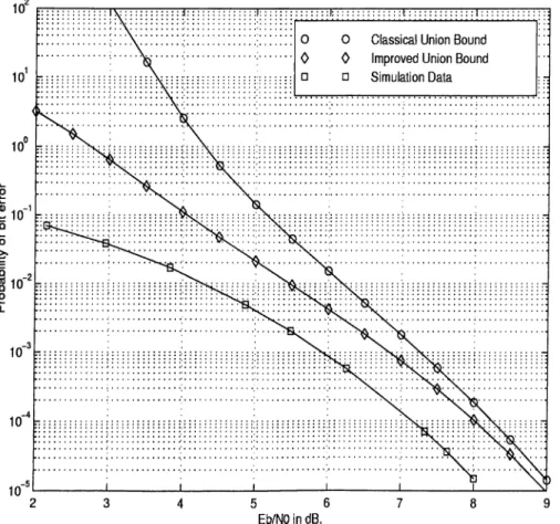
In this section, results for the rate-1/ 2, constraint-length-3 code will be presented. Im­ proved bound will be compared to simulations and to the classical union bound as given by Viterbi.

Simulations are performed using a Viterbi software decoder written in C language. Though the final program is extensively modified for use with different channel charac­ teristics and with codes of different constraint length, the basic modules are based on Robert Morelos Zaragoza’s Viterbi decoder program [19].

It is usually difficult to get a good statistical sample especially for very low error rates. The experiments are performed over 10® —10® bits blocks and are repeated several times to ensure th at the mean value lies in an acceptable confidence interval. For experiments of this section all data points, Xf lie in an interval of Axj = O.Olxj with 95% probability.

First, a BSC with BPSK modulation will be considered. The crossover probability in this case is given by ____

1

P = iREt_{N. )} (3.18)

where R denotes the rate of the code and Ei, / Nq is the SNR at the system input. Therefore, in Eq. 3.6 and Eq. 3.7, To(l) = P and Po(0) = q = 1 - p.

For this case, experiments show that truncating the length of possible paths at L^ax = 30 which is 10-times the constraint length provide sufficient accuracy. The maximization in Eq. 3.3 is performed numerically. In Fig. 3.3, the results are plotted for a range of SNR values and compared to classical union bound and to simulation data. Simulation data