Perspective projections in the space-frequency
plane and fractional Fourier transforms
I˙. S¸amil Yetik, Haldun M. Ozaktas, Billur Barshan, and Levent Onural Department of Electrical Engineering, Bilkent University, TR-06533 Bilkent, Ankara, Turkey Received March 16, 2000; revised manuscript received July 6, 2000; accepted July 10, 2000
Perspective projections in the space-frequency plane are analyzed, and it is shown that under certain condi-tions they can be approximately modeled in terms of the fractional Fourier transform. The region of validity of the approximation is examined. Numerical examples are presented. © 2000 Optical Society of America [S0740-3232(00)00612-8]
OCIS codes: 100.0100, 150.0150.
1. INTRODUCTION
Perspective projections are used in many applications in image and video processing, especially when one is con-fronted with natural or artificial scenes with depth (for in-stance, in robot vision applications). Perspective projec-tion can be considered as a geometric or pointwise transformation in the sense that each point of the object is mapped to another point in the perspective projection.1–3 In this paper we examine the perspective projection in the space-frequency plane and show that its effect on the object can be modeled in terms of the frac-tional Fourier transform.
A widely employed space-frequency representation is the Wigner distribution, defined as
Wf共x, x兲 ⫽
冕
f共x ⫹ x⬘/2兲f*共x ⫺ x⬘/2兲⫻ exp共⫺i2xx⬘兲dx⬘. (1)
The Wigner distribution provides information regarding the distribution of the signal energy over space and fre-quency. Especially important among its properties are the following relations:
冕
Wf共x, x兲dx⫽ 兩f共x兲兩2, (2)冕
Wf共x, x兲dx ⫽ 兩F共 x兲兩2, (3)冕冕
Wf共x, x兲dxdx⫽ 储f 储2⫽ En关f 兴 ⫽ signal energy.(4) The Wigner distribution of an exponential function exp(i2 x) is a line delta lying parallel to the space axis: Wf共x, x兲 ⫽␦共 x⫺兲, (5)
and the Wigner distribution of a chirp function exp关i (x2⫹ 2 x ⫹ )兴 is an oblique line delta:
Wf共x, x兲 ⫽␦共 x⫺x ⫺ 兲. (6)
Further discussion regarding the properties of the Wigner distribution may be found in Ref. 4.
The fractional Fourier transform is a generalization of the ordinary Fourier transform with a fractional order pa-rameter a. It has found many applications in optics and signal processing.5–30 We refer the reader to Ref. 5 for a comprehensive treatment and further references and to Ref. 7 for a more concise introduction. Here we briefly mention a few important properties. The ath-order frac-tional Fourier transform fa(u) is a unitary transform
de-fined as
fa共x兲 ⫽
冕
Ka共x, x⬘兲f共x⬘兲dx⬘,Ka共x, x⬘兲 ⫽ Aaexp兵i关cot共a/2兲x2
⫺ 2 csc共a/2兲xx⬘⫹ cot共a/2兲x⬘2兴其, (7) where Aa is a constant that depends on a. The
zeroth-order fractional Fourier transform corresponds to the identity operation, and the first-order fractional Fourier transform corresponds to the ordinary Fourier transform. Furthermore, the fractional Fourier transform is index additive; that is, the a1th-order fractional Fourier trans-form of the a2th-order fractional Fourier transform is equal to the (a1⫹ a2)th-order fractional Fourier trans-form. The ath-order fractional Fourier transform corre-sponds to a clockwise rotation of the Wigner distribution by an angle␣ ⫽ a/2 in the space-frequency plane:
Wfa共x, x兲 ⫽ Wf共x cos␣ ⫺ xsin␣, x sin ␣ ⫹ xcos␣兲.
(8) The fractional Fourier transform has a fast implementa-tion with complexity O(N log N).5,7
To understand why the fractional Fourier transform is expected to play a role in perspective projections, let us consider the perspective projection of an image exhibiting periodic features, such as a railroad track. More distant parts of the image will appear smaller in the projection than closer parts will. Thus a periodic or harmonic fea-ture of a certain frequency will be mapped such that it ex-hibits a monotonically increasing frequency. Under cer-tain conditions this increase can be assumed linear so that the harmonic function is mapped to a chirp function. Since fractional Fourier transforms are known to map
harmonic functions to chirp functions, we expect that per-spective projections can be modeled in terms of fractional Fourier transforms. The purpose of this paper is to for-mulate this relationship.
In Section 2 we present the perspective model that we use and examine the effect of the perspective projection on the Wigner distribution. In Section 3 we discuss the relationship between the fractional Fourier transform and perspective projections based on their effects on the Wigner distribution. We also discuss how perspective projections can be modeled as shifted and fractional Fou-rier transformations. Section 4 is devoted to an analysis of the errors and the region of validity of the approxima-tions.
2. PERSPECTIVE PROJECTION
The perspective model that we use is shown in Fig. 1. Initially, we consider perspective projections for one-dimensional (1D) signals, since this approach signifi-cantly simplifies the presentation. The horizontal axis, labeled x, represents the original object space. The ver-tical axis, labeled xp, represents the perspective
projec-tion space. The point A with coordinates (⫺x0, xp0) is
the center of projection. We denote the original signal (object) by f(x) and its perspective projection by g(xp).
We assume that most of the energy of f(x) is confined to the interval [x¯ ⫺ ⌬x/2, x¯ ⫹ ⌬x/2]. In the frequency do-main we assume that most of the energy of F(x), the
Fourier transform of f(x), is confined to the interval [¯x
⫺ ⌬x/2, ¯x⫹ ⌬x/2]. The value of f(x) at each x is
mapped to the coordinate xp, which is the projection of
the point x: xp⫽ xxp0 x⫹ x0 , (9) x⫽ x0xp xp0⫺ xp , (10)
which can be derived by simple geometry. Thus the pro-jection g(xp) is expressed as follows:
g共xp兲 ⫽ f
冉
x0xp
xp0 ⫺ xp
冊
. (11)
The interval to which most of the energy of g(xp) is
ap-proximately confined can be determined from Eq. (9).
To see the effect of perspective projections in the space-frequency plane, we decompose f(x) into harmonics as fol-lows:
f共x兲 ⫽
冕
F共 x兲exp共i2xx兲dx, (12)where F(x) is the Fourier transform of f(x). Using Eq.
(11) and the rules of linearity, we obtain the following ex-pression for g(xp): g共xp兲 ⫽
冕
F共 x兲h共xp,x兲dx, (13) where h共xp,x兲 ⫽ exp冋
i2x冉
x0xp xp0⫺ xp冊
册
dx. (14)We will initially concentrate on a single exponential with frequency¯xand study the effect of perspective projection
in the space-frequency plane. Then we will construct g(xp) by first decomposing f(x) in terms of exponentials
and using Eq. (13).
The Wigner distribution of h(xp,¯x) cannot be
explic-itly obtained. Therefore, to continue our analytical de-velopment, we expand the phase of h(xp,¯x) into a
Tay-lor series. We will expand the phase of h(xp,¯x) around
the point to which x¯ is mapped: x ¯ x ¯ ⫹ x0
xp0, (15)
which we express as xp0, where ⫽ x¯/(x¯ ⫹ x0). Ex-panding the phase of h(xp, ¯x) aroundxp0, we obtain
the following equation after performing some algebra: h共xp, ˜x兲 ⫽ exp
再
i2xx0冋
xp2 共1 ⫺兲3x p02 ⫹ xp共1 ⫺ 3兲 共1 ⫺兲3x p0 ⫹ 3 共1 ⫺兲3 ⫹ ...册
冎
. (16)Ignoring terms higher than the second order, we can see that the projection of a harmonic is a chirp function. The validity of this approximation requires that the third-order term be much smaller than the second-third-order term: 兩 ⫹ 2兩 Ⰶ 兩2xp0共 ⫺ 1兲兩. (17)
This approximation is more accurate for larger values of xp0. This is expected, since larger xp0values correspond
to perspective projections that are not as deep. The Wigner distribution of the chirp given in Eq. (16) is a line delta given by ␦
冋
x⫹ 2¯x 共1 ⫺兲3x p02 xp⫹ ¯x共1 ⫺ 3兲 共1 ⫺兲3x p0册
(18) and is shown in Fig. 2(b) below.Having obtained an approximate analytical form for the perspective projection of a harmonic as well as an ap-proximate expression for the perspective projection’s Wigner distribution, we now move on to our discussion of
Fig. 1. Perspective model: f(x) represents the object
distribu-tion on the x axis; g(xp) represents its perspective projection onto the xpaxis. The point A with coordinates (⫺x0, xp
0) is the
perspective projections in the space-frequency plane and of their relationship to the fractional Fourier transform.
3. RELATIONSHIP BETWEEN PERSPECTIVE
PROJECTIONS AND FRACTIONAL
FOURIER TRANSFORMS
In Section 2 we obtained an approximate expression for the Wigner distribution of the perspective projection of a single exponential. The Wigner distribution of a typical exponential and the Wigner distribution of the approxi-mate perspective projection of the exponential are shown in Fig. 2. The angle that the line delta makes with the x axis is arctan兵2¯x/关(1 ⫺)3xp0
2兴其 which depends on ¯
x.
The fact that the oblique line delta is a rotated version of the horizontal line delta suggests a role for the fractional Fourier transform, since this operation corresponds to ro-tation in the space-frequency plane.
We will now show how the perspective projection of a signal can be approximately expressed in terms of the fractional Fourier transform. We claim that the perspec-tive projection of a signal can be obtained from, or mod-eled by, the following steps:
1. Shift the signal by x¯ in the negative x direction and by ¯x in the negative x direction. This translates the
Wigner distribution of the signal to the origin of the space-frequency plane.
2. Take the fractional Fourier transform with the or-der a ⫽ (⫺2/)arctan兵关2¯x(x¯⫹ x0)3兴/xp02x02其. This ro-tates the Wigner distribution by an angle a/2.
3. Shift the result by x¯ xp0/(x¯ ⫹ x0) in the positive x
direction and by关¯x(x¯ ⫹ x0)2兴/x0xp0in the positivex
di-rection.
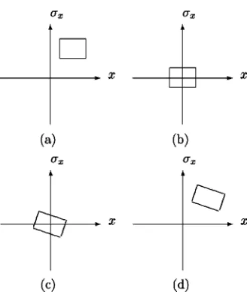
These steps represent a decomposition of the overall ef-fect of the perspective projection, from which we can see that to perform perspective projection is essentially to ef-fect a rotation in the space-frequency plane. However, this rotation is enacted on the space-frequency content of the signal that is referred to the origin of the space-frequency plane. The above steps are illustrated in Fig. 3.
Different frequency components of the signal require different fractional Fourier orders, because the order a given in step 3 depends on ¯x. However, as we will
show, under certain conditions a satisfactory approxima-tion can be obtained by use of a uniform order correspond-ing to the central frequency of the signal.
We now demonstrate our claim that perspective projec-tion can be decomposed into the three steps given above. We start by decomposing f(x) into harmonics:
f共x兲 ⫽
冕
F共 x兲exp共2ixx兲dx. (19)We will concentrate on a single-harmonic component, exp(i2xx), and the result for general f(x) will follow by
linearity. Applying step 1 to a single harmonic, we ob-tain
exp共i2x¯x兲. (20)
Now we apply steps 2 and 3 to this result to obtain
Fig. 2. (a) Wigner distribution of the original exponential. (b) Wigner distribution of the approximate perspective projection: a chirp.
Fig. 3. Illustration of the decomposition of the approximation into elementary operations in the space-frequency plane: (a) Original signal, (b) after step 1 (space and frequency shift), (c) af-ter step 2 (fractional Fourier transform), (d) afaf-ter step 3 (space and frequency shift): approximate perspective projection.
冉
1 ⫹ i2x¯x⫹ x0 xp02x03冊
1/2 exp共i2x¯x兲 ⫻ exp冋冉
i2x2 x x ¯ ⫹ x0 xp0 2x 03冊
册
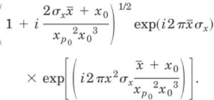
. (21)Last, we apply step 4 and obtain our final result:
冋
1 ⫹ i2x共x¯ ⫹ x0兲 3 xp0 2x 03册
1/2 exp共i2x¯x兲 ⫻ exp冋
i2x冉
x⫺ x ¯ xp0 x ¯⫹ x0冊
2冉
¯x⫹ x0 xp02x03冊
册
⫻ exp冋
i4x冉
x ¯⫹ x02 x02xp0冊
册
. (22)Multiplying this by F(x) and integrating overxyields
the desired approximate expression for the perspective projection of f(x), which is the mathematical expression of the four steps outlined above.
To see that this expression is indeed an approximation of the perspective projection, we again concentrate on a single-harmonic component whose exact perspective pro-jection is
exp
冉
2ixx0xp
xp0⫺ xp
冊
. (23)
Using the Taylor-series expansion, we obtain
exp
再
i2xx0冋
xp2 共1 ⫺兲3x p0 2 ⫹ xp共1 ⫺ 3兲 共1 ⫺兲3x p0 ⫹ 3 共1 ⫺兲3册
冎
, (24)which differs from expression (22) only by a constant fac-tor. As far as a single-harmonic component is concerned, the only approximation that is involved is the binomial expansion in the exponent. When the harmonic compo-nents are superposed to yield the original function f(x), we make the additional approximation of using the order corresponding to the center frequency for all the harmonic components. Thus our three-step procedure will deviate from the exact perspective projection more and more as the bandwidth of f(x) is increased. The limitations asso-ciated with this approximation are discussed in Section 4. Figure 4 shows the exact perspective projection of the function
cos共4x兲rect
冉
x⫺ 4 6冊
⫽冋
exp共i4x兲 ⫹ exp共⫺i4x兲
2
册
⫻ rect
冉
x⫺ 46
冊
(25)superimposed upon the approximation given by expres-sion (24). We chose x0⫽ ⫺3, xp0⫽ 6 as the center of
projection. As a second example, we consider the
narrow-band signal shown in Fig. 5. Here, too, the exact perspective projection and the fractional Fourier approxi-mation are superimposed [see Fig. 5(b)]. We observe that the approximation is quite satisfactory except for very near the edges, which should be avoided.
Generalization of the proposed method to two dimen-sions is possible if similar steps are followed. In our two-dimensional (2D) perspective model we use a 2D image with midpoints x¯ , y¯ ; center frequencies¯x, ¯y; and
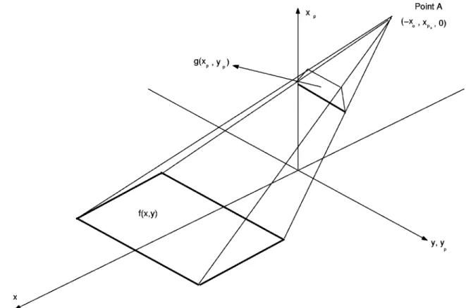
spa-tial widths⌬x, ⌬y. Our center of projection is located at (x0, xp0, 0). The model described is shown in Fig. 6.
With this model, using simple geometry, we can obtain the following mappings and reverse mappings for each xp
and yp:
Fig. 4. (a) Original signal. (b) Exact perspective projection (solid curve) superimposed upon the fractional Fourier approxi-mation (dashed curve).
Fig. 5. (a) Original signal. (b) Exact perspective projection (solid curve) superimposed upon the fractional Fourier approxi-mation (dashed curve).
xp⫽ xxp0 x⫹ x0 , (26) x⫽ x0xp xp0⫺ xp , (27) yp⫽ x⌬y ⫹ 2x0y 2共x ⫹ x0兲 , (28) y⫽ ypxp0 xp0⫺ xp ⫺ xp⌬y 2共x0⫺ xp兲 . (29)
As in the 1D case, we first decompose f(x, y) into harmon-ics:
f共x, y兲 ⫽
冕
F共 x,y兲exp共i2xx兲exp共i2yy兲dxdy.(30)
We proceed by writing an expression for the perspective projection of a 2D harmonic, exp(i2¯xx)exp(i2¯yy):
exp
再
i2¯xx0冋
xp2 共1 ⫺兲3x p02 ⫹ xp共1 ⫺ 3兲 共1 ⫺兲3x p0 ⫹ 3 共1 ⫺兲3册
冎
, ⫻ exp再
⫺i¯y⌬y冋
xp2 共1 ⫺⬘兲3x 02 ⫹ xp共1 ⫺ 3⬘兲 共1 ⫺⬘兲3x 0 ⫹ ⬘ 3 共1 ⫺⬘兲3
册冎
, ⫻ exp再
i2¯yyp冋
xp2 xp0 2共1 ⫺兲3 ⫹ xp共1 ⫺ 3兲 xp共1 ⫺兲3 ⫹ 3 2⫺ 3 ⫹ 1 共 ⫺ 1兲3册
冎
, (31)where again the binomial approximation has been em-ployed and ⫽ x¯/(x¯ ⫹ x0) and⬘⫽ x¯/(x¯ ⫹ ⌬y). Close examination of expression (31) reveals that we have the product of a 1D chirp in the xpdirection and a scaled
har-monic in the ypdirection whose scaling factor depends on
xp. We are going to approximate the perspective
projec-tion by using 1D shifts and 1D fracprojec-tional Fourier trans-forms followed by scaling. We claim that the 2D perspec-tive projection of a signal can be obtained from, or modeled by, the following steps:
Fig. 6. Perspective model: f(x, y) represents the object distribution on the x – y plane; g(xp, yp) represents the object distribution’s perspective projection onto the xp– ypplane. The point A with coordinates (⫺x0, xp0, 0) is the center of projection.
1. Shift the signal by x¯ in the negative x direction and by ¯x in the negative x direction. This translates the
Wigner distribution of the signal to the origin of the space-frequency plane.
2. Take the 1D fractional Fourier transforms in the variable x with order
a⫽ ⫺2 arctan
冋
2¯x共x¯ ⫹ x0兲3 xp02x02 ⫺ 共x¯ ⫹ ⌬y兲 3¯ y ⌬y2x 02册
,treating y as a parameter. This rotates the Wigner dis-tributions by an angle a/2.
3. Shift the result by x¯ xp0/(x¯ ⫹ x0) in the positive x
direction and by
冋
¯x共x¯ ⫹ x0兲3 xp0x0 ⫺ 共x¯ ⫹ ⌬y兲 3¯ y ⌬y2x 02册
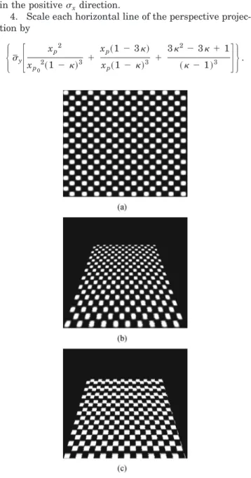
in the positivexdirection.4. Scale each horizontal line of the perspective projec-tion by
再
¯y冋
xp2 xp02共1 ⫺兲3 ⫹ xp共1 ⫺ 3兲 xp共1 ⫺兲3 ⫹ 3 2⫺ 3 ⫹ 1 共 ⫺ 1兲3册
冎
.The mathematical combination of the above steps yields the 2D perspective projection of a 2D harmonic, given by expression (31). Multiplying this by F(x,y) and
inte-grating overxandyyields the desired approximate
ex-pression for the perspective projection of f(x, y), which is the mathematical expression of the four steps outlined above. An example is given in Fig. 7, where the fractional-Fourier-transform-based result shown in Fig. 7(c) can be seen to be a reasonable approximation of the actual perspective projection shown in Fig. 7(b).
4. ERROR ANALYSIS
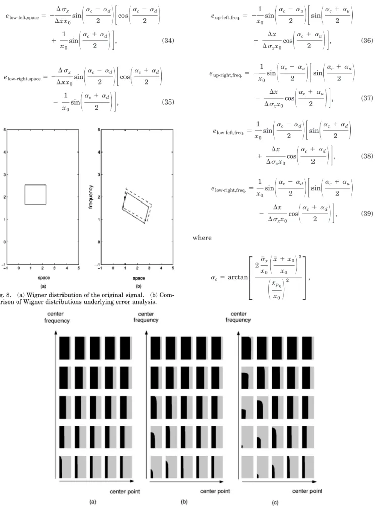
In this section we examine the conditions under which the fractional Fourier transform approximation to the per-spective projection is valid. We first examine the modifi-cations that the Wigner distribution undergoes corre-sponding to the approximation. Since we know that the approximation can be decomposed into the four steps given in Section 3, it is easy to find the resulting changes in the Wigner distribution. To estimate the error inher-ent in our approximation, we will think of the original Wigner distribution as consisting of horizontal strips of narrow frequency components. The major approxima-tion that we make is to replace the fracapproxima-tional orders re-quired by these different frequency components with a single order corresponding to the central frequency. To determine the error introduced by this approximation, we first determine how the highest- and the lowest-frequency strips would be mapped had their individual frequencies been used instead of the center frequency. Let us as-sume that most of the energy of the Wigner distribution of a signal is concentrated in a rectangular region in the space-frequency plane [Fig. 8(a)]. Figure 8(b) shows the Wigner distribution corresponding to the fractional Fou-rier approximation (solid lines). The dashed lines, in contrast, show the Wigner contour obtained by using the individual frequencies for the highest- and the lowest-frequency strips.
Our error criteria will be the deviations of the corners of the two superimposed Wigner contours shown in [Fig. 8(b)]. There will be one spatial deviation and one fre-quency deviation for each of the four corners of the con-tours. We will normalize the spatial deviation by⌬x and the frequency deviations by ⌬xand take the maximum
of the resulting eight normalized deviations as our final error measure. Expressions for the eight normalized de-viations are given below:
eup-left,space⫽ ⌬x ⌬xx0 sin
冉
␣c⫺␣u 2冊冋
cos冉
␣c⫹␣u 2冊
⫹ 1 x0 sin冉
␣c⫹ ␣u 2冊册
, (32) eup-right,space⫽ ⌬x ⌬xx0 sin冉
␣c⫺ ␣u 2冊冋
cos冉
␣c⫹␣u 2冊
⫺ 1 x0 sin冉
␣c⫹␣u 2冊册
, (33)Fig. 7. (a) Original signal. (b) Exact perspective projection. (c) Fractional Fourier approximation.
elow-left,space⫽ ⫺ ⌬x ⌬xx0 sin
冉
␣c⫺␣d 2冊冋
cos冉
␣c⫺ ␣d 2冊
⫹ 1 x0 sin冉
␣c⫹␣d 2冊册
, (34) elow-right,space⫽ ⫺ ⌬x ⌬xx0 sin冉
␣c⫺␣d 2冊冋
cos冉
␣c⫹␣d 2冊
⫺ 1 x0 sin冉
␣c⫹␣d 2冊册
, (35) eup-left,freq.⫽ ⫺ 1 x0 sin冉
␣c⫺ ␣u 2冊冋
sin冉
␣c⫹␣u 2冊
⫹ ⌬x ⌬xx0 cos冉
␣c⫹␣u 2冊册
, (36) eup-right,freq.⫽ ⫺ 1 x0 sin冉
␣c⫺␣u 2冊冋
sin冉
␣c⫹␣u 2冊
⫺ ⌬x ⌬xx0 cos冉
␣c⫹ ␣u 2冊册
, (37) elow-left,freq.⫽ 1 x0 sin冉
␣c⫺␣d 2冊冋
sin冉
␣c⫹␣d 2冊
⫹ ⌬x ⌬xx0 cos冉
␣c⫹ ␣d 2冊册
, (38) elow-right,freq.⫽ 1 x0 sin冉
␣c⫺ ␣d 2冊冋
sin冉
␣c⫹ ␣u 2冊
⫺ ⌬x ⌬xx0 cos冉
␣c⫹␣d 2冊册
, (39) where ␣c⫽ arctan冋
2¯x x0冉
x ¯⫹ x0 x0冊
3冉
xp0 x0冊
2册
,Fig. 8. (a) Wigner distribution of the original signal. (b) Com-parison of Wigner distributions underlying error analysis.
Fig. 9. Dark shading: parameter combinations whose normalized error is less than 10%. Light shading: region in which the error is large. See text for details.
␣u⫽ arctan
冋
2冉
¯x x0 ⫹ ⌬x 2x0冊冉
x ¯ ⫹ x0 x0冊
3冉
xp0 x0冊
2册
, ␣d⫽ arctan冋
2冉
¯x x0⫺ ⌬x 2x0冊冉
x ¯ ⫹ x0 x0冊
3冉
xp0 x0冊
2册
.To reduce the number of parameters by one, we have ex-pressed the above results so that all the free parameters appear divided by x0.
It does not seem possible to analytically derive conclu-sions by use of these formulas, so we will resort to nu-merically obtained plots. The approximation will be as-sumed to be acceptable if the maximum normalized error is less than 10%. The expressions given above yield the error as a function of six variables: x0, xp0, x¯ , ¯x,
⌬x, ⌬x. However, normalizing all the variables by x0, we can reduce the number of variables to five. In Fig. 9 we show as dark regions the region in which the maxi-mum normalized error is less than 10%, whereas the light regions indicate that in which the error is large. The horizontal axis in each of the 75 plots represents the value of⌬x/x0, and the vertical axis represents⌬x/x0. Both these variables range from 101/30to 10100/30in these log–log plots.
Each member of the 5 ⫻ 5 matrices of plots corre-sponds to different values of x¯ /x0(horizontal),¯x/x0 (ver-tical). The five separate values of x¯ /x0 are 10⫺1/2, 100/2, 101/2, 102/2, 103/2, and the five separate values of¯
x/x0are 10⫺1/2, 100/2, 101/2, 102/2, 103/2. The three groups of 25 plots each correspond to different values of the center of projection: xp0/x0⫽ 0.1 [Fig. 9(a)], xp0/x0⫽ 1 [Fig.
9(b)], xp0/x0⫽ 10 [Fig. 9(c)].
This set of plots covering a broad range of the param-eter values allows us to dparam-etermine whether the approxi-mation developed is acceptable for a certain range of pa-rameters. Generally speaking, we have larger acceptable regions for larger values of¯x. Not surprisingly, the
ap-proximation is strained as⌬x and ⌬x increase, i.e., as
the space–bandwidth product of the signal increases.
5. CONCLUSION
In this paper we examined perspective projections in the space-frequency plane and showed how to approximate the perspective projection in terms of the fractional Fou-rier transform. Our main motivation was to show that the fractional Fourier transform approximately captures the essence of the warping characteristic of perspective projections. We observed that perspective projection ap-proximately maps harmonic components into chirps and that it can therefore be modeled in terms of the fractional Fourier transform. We saw that the substance of per-spective projection is essentially to effect a rotation in the space-frequency plane. However, this rotation is enacted on the space-frequency content of the signal referred to the origin of the space-frequency plane. Elementary
nu-merical examples for both one-dimensional signals and two-dimensional images were presented. The errors as-sociated with the approximation and the region of validity with respect to the approximations involved were numeri-cally discussed.
I˙. S¸ . Yetik can be reached by e-mail at [email protected].
REFERENCES
1. D. Vernon, Machine Vision: Automated Visual Inspection and Robot Vision (Prentice-Hall, New York, 1991). 2. A. Low, Introductory Computer Vision and Image
Process-ing (McGraw-Hill, New York, 1991).
3. G. Woldberg, Digital Image Warping (IEEE Computer So-ciety, Los Alamitos, Calif., 1992).
4. L. Cohen, Time-Frequency Analysis (Prentice-Hall PTR, Englewood Cliffs, N.J., 1995).
5. H. M. Ozaktas, Z. Zalevsky, and M. A. Kutay, The Frac-tional Fourier Transform with Applications in Optics and Signal Processing (Wiley, New York, 2000).
6. H. M. Ozaktas, B. Barshan, D. Mendlovic, and L. Onural, ‘‘Convolution, filtering, and multiplexing in fractional Fou-rier domains and their relation to chirp and wavelet trans-forms,’’ J. Opt. Soc. Am. A 11, 547–559 (1994).
7. H. M. Ozaktas, M. A. Kutay, and D. Mendlovic, ‘‘Introduc-tion to the frac‘‘Introduc-tional Fourier transform and its applica-tions,’’ Adv. Imaging Electron Phys. 106, 239–291 (1999). 8. L. B. Almeida, ‘‘The fractional Fourier transform and
time-frequency representations,’’ IEEE Trans. Signal Process. 42, 3084–3092 (1994).
9. S. Abe and J. T. Sheridan, ‘‘Comment on ‘ The fractional Fourier transform in optical propagation problems,’ ’’ J. Mod. Opt. 42, 2373–2378 (1995).
10. O. Akay and G. F. Boudreaux-Bartels, ‘‘Unitary and Her-mitian fractional operators and their relation to the frac-tional Fourier transform,’’ IEEE Signal Process. Lett. 5, 312–314 (1998).
11. T. Alieva, ‘‘Fractional Fourier transform as a tool for inves-tigation of fractal objects,’’ J. Opt. Soc. Am. A 13, 1189– 1192 (1996).
12. T. Alieva and F. Agullo-Lopez, ‘‘Diffraction analysis of ran-dom fractal fields,’’ J. Opt. Soc. Am. A 15, 669–674 (1998). 13. L. M. Bernardo and O. D. D. Soares, ‘‘Fractional Fourier transforms and imaging,’’ J. Opt. Soc. Am. A 11, 2622–2626 (1994); Y. Bitran, Z. Zalevsky, D. Mendlovic, and R. G. Dorsch, ‘‘Fractional correlation operation: performance analysis,’’ Appl. Opt. 35, 297–303 (1996).
14. W. X. Cong, N. X. Chen, and B. Y. Gu, ‘‘Beam shaping and its solution with the use of an optimization method,’’ Appl. Opt. 37, 4500–4503 (1998).
15. R. G. Dorsch and A. W. Lohmann, ‘‘Fractional Fourier transform used for a lens design problem,’’ Appl. Opt. 34, 4111–4112 (1995).
16. D. Dragoman and M. Dragoman, ‘‘Near and far field optical beam characterization using the fractional Fourier trans-form,’’ Opt. Commun. 141, 5–9 (1997).
17. M. F. Erden, M. A. Kutay, and H. M. Ozaktas, ‘‘Repeated filtering in consecutive fractional Fourier domains and its application to signal restoration,’’ IEEE Trans. Signal Pro-cess. 47, 1458–1462 (1999).
18. J. Garcı´a, D. Mendlovic, Z. Zalevsky, and A. Lohmann, ‘‘Space-variant simultaneous detection of several objects by the use of multiple anamorphic fractional-Fourier-transform filters,’’ Appl. Opt. 35, 3945–3952 (1996). 19. S. Granieri, O. Trabocchi, and E. E. Sicre, ‘‘Fractional
Fou-rier transform applied to spatial filtering in the Fresnel do-main,’’ Opt. Commun. 119, 275–278 (1995).
20. C. J. Kuo and Y. Luo, ‘‘Generalized joint fractional Fourier transform correlators: a compact approach,’’ Appl. Opt. 37, 8270–8276 (1998).
21. M. A. Kutay and H. M. Ozaktas, ‘‘Optimal image restora-tion with the fracrestora-tional Fourier transform,’’ J. Opt. Soc. Am. A 15, 825–833 (1998).
22. M. A. Kutay, H. M. Ozaktas, O. Arikan, and L. Onural, ‘‘Op-timal filtering in fractional Fourier domains,’’ IEEE Trans. Signal Process. 45, 1129–1143 (1997).
23. A. W. Lohmann, D. Mendlovic, and Z. Zalevsky, ‘‘Fractional transformations in optics,’’ in Progress in Optics, XXXVIII, E. Wolf, ed. (Elsevier, Amsterdam, 1998), Chap. 4, pp. 263– 342.
24. S. Mann and S. Haykin, ‘‘The chirplet transform: physical considerations,’’ IEEE Trans. Signal Process. 43, 2745– 2761 (1995).
25. D. Mendlovic, Z. Zalevsky, A. W. Lohmann, and R. G. Dorsch, ‘‘Signal spatial-filtering using the localized
frac-tional Fourier transform,’’ Opt. Commun. 126, 14–18 (1996).
26. V. Namias, ‘‘The fractional order Fourier transform and its application to quantum mechanics,’’ J. Inst. Math. Appl. 25, 241–265 (1980).
27. H. M. Ozaktas and O. Aytu¨ r, ‘‘Fractional Fourier domains,’’ Signal Process. 46, 119–124 (1995).
28. Z. Zalevsky and D. Mendlovic, ‘‘Fractional Wiener filter,’’ Appl. Opt. 35, 3930–3936 (1996).
29. Z. Zalevsky, D. Mendlovic, and J. H. Caulfield, ‘‘Localized, partially space-invariant filtering,’’ Appl. Opt. 36, 1086– 1092 (1997).
30. Y. Zhang, B.-Z. Dong, B.-Y. Gu, and G.-Z. Yang, ‘‘Beam shaping in the fractional Fourier transform domain,’’ J. Opt. Soc. Am. A 15, 1114–1120 (1998).