Polarization independent thermo-optic modulators for integrated optics

(1)

POLARIZATION INDEPENDENT

THERMO-OPTIC MODULATORS FOR

INTEGRATED OPTICS

a thesis

submitted to the department of physics and the institute of engineering and science

of b˙Ilkent university

in partial fulfillment of the requirements for the degree of

master of science

By

A¸skın Kocaba¸s

September 2003

(2)

I certify that I have read this thesis and that in my opinion it is fully adequate, in scope and in quality, as a dissertation for the degree of Master of Science.

Prof. Atilla Aydınlı (Supervisor)

Assoc. Prof. Ahmet Oral

Asst. Prof. Soner Kılı¸c

Approved for the Institute of Engineering and Science:

Prof. Mehmet Baray,

(3)

(4)

Abstract

POLARIZATION INDEPENDENT THERMO-OPTIC

MODULATORS FOR INTEGRATED OPTICS

A¸skın Kocaba¸s

M. S. in Physics

Supervisor: Prof. Atilla Aydınlı

September 2003

In this work, we studied MMI and Y-junction based Mach-Zehnder modulators on both silicon-on-insulator and polymer based on thermo-optic effect. Both Pπ values and frequency response of the devices were measured

and found to be consistent with those observed in the literature as well as results obtained from finite element simulations. We feel that our BCB based Y-junction modulators have the highest reported 3 -dB cut-off frequency to date. We also observe that all of our devices are polarization independent, an important feature for applications in optical communications.

Keywords: Thermo-optic modulators, Thermo-optic effect, Finite element method, Multi-mode interference, Y-junction modulator, Poly-mer modulator. .

(5)

(6)

¨

Ozet

T ¨

UMLES¸˙IK OPT˙IK UYGULAMALARI ˙IC

¸ ˙IN KUTUPSAL

OLMAYAN ISIL OPT˙IK K˙IPLEY˙IC˙ILER

A¸skın Kocaba¸s

Fizik Y¨uksek Lisans

Tez Y¨oneticisi: Prof. Atilla Aydınlı

Eyl¨ul 2003

Bu tezde, ısıl optik etkiye dayanan, MMI ve Y-eklem ¸ciftleyicilere dayalı sil-isyum ve polimer kipleyiciler ¸calı¸sıldı. Kipleyicilerin Pπ deˇgerleri ve frekansa g¨ore

tepkileri öl¸cüldü, ve elde edilen deˇgerlerin hem sonlu eleman metoduyla elde edilen benze¸sim sonu¸cları hem de bilimsel yazındaki deˇgerlerle uygun olduˇgu görüldü. Polimer kipleyici i¸cin bulunan 3-dB kesim deˇgerinin ¸su ana kadar öl¸cülmü¸s en yüksek deˇger olduˇgu gözlendi. Bu kipleyicilerin kutupsal olmadıkları da gözlendi.

Anahtar

sözcükler: Isıl-optik kipleyici, Isıl-optik etki, Sonlu elemanlar metodu, Ç ok kipli giri¸sim, Y-eklem kipleyici, Polimer kipleyici.

(7)

(8)

Acknowledgement

I would like to express my deepest gratitude to Prof. Atilla Aydınlı for his guidance, moral support, friendship and assistance during this research.

I would like to thank my twin brother Co¸skun for his help that has been invaluable for me.

I would like to thank ˙Imran AKC¸ A for her help during optical measurements and especially for FEM Simulations of thermo-optic devices.

I would like to thank ˙Isa Kiyat his help for optical measurements and design of the MMI devices.

I would like to thank Feridun Ay for DPM measurements and critical reading of the manuscript.

I would like to thank Asst. Prof. Soner Kılı¸c for his guidance in preparing the polymer films.

I would like to thank to all Integrated Optics Group members Selcen Aytekin, Hasan ˙I¸slek, Mahmut Demir, and Nuh Sadi Y¨uksek for their friendship and to keep my sprits high.

Turgut Tut, Ayhan Yurtsever, Sinem Binicioˇglu, Ertuˇgrul Ç ubuk¸cu, Engin Durgun, Deniz Ç akir, Cem Sevik, Ercan Avcı, Mustafa Kesir, Süleyman Tek, Necmi Bıyıklı helped to keep my spirits high all the time which I appreciate very much.

I am indebted to my family for their continuous support and care.

(9)

List of Figures

2. 1 Oscillations of temperature caused by periodic boundary condi-tions in a material with different thermal properties. . . 13 2. 2 Simulation steps in FEM (a)Drawing (b)Meshing (c) Solution. . . 16 3. 1 Different types of optical waveguides . . . 18 3. 2 EIM analysis of a rib waveguide . . . 18 3. 3 Schematic diagram of MMI coupler. . . 20 3. 4 Example of amplitude normalized lateral field profiles

correspond-ing to step-index multi-mode waveguide. . . 21 3. 5 a)Multi-mode waveguide showing the input field, mirrored single

image, a direct single image, and two fold images. b)BPM simulation of multi-mode waveguide to illustrate the image formation. . . 22 3. 6 Schematic diagram of MMI modulator. . . 25 3. 7 BPM simulation of MMI modulator for off (a) and on state (b). . 26 3. 8 Sidewiev of MMI modulator . . . 27 3. 9 Single mode condition for different Si top layer thicknesses. For

H=4 um, waveguide width of 3 um requires the etch depth to obtain the rib as 1.4 um . . . 28 3. 10(a)Schematic diagram of waveguide structure, (b) TE fundamental

mode shape for Si ridge waveguide as calculated by BPM. . . 29 3. 112D steady state temperature distribution of the MMI modulator.

The power applied to the electrode is 114 mW, . . . 30

(12)

3. 12Simulation results of pulse response when 1 kHz square wave is applied to electrode. (a)applied power (b)temperature response

(c)output light intensity. . . 31

3. 13Simulation result for modulation depth of output light intensity as a function of frequency. . . 32

3. 14All Patterning steps of SOI optical waveguides, (a)SOI structure, (b)Si3N4 Deposition, (c)Photoresist Spinning, (d)Photolithography, (e)HF Etching, (f)KOH Etching, (g)Removing Si3N4 . . . 34

3. 15Trench patterning steps of SOI optical waveguides (a) Si MMI waveguide, (b) Si3N4 Deposition, (c) Defining trench pattern, (d) KOH Etching, (e) Removing Si3N4, (f) SEM photograph of MMI modulator . . . 36

3. 16Electrode metallization of thin film heaters (a) Patterned Si waveg-uide, (b) Spinning PR, (c) Defining heater, (d) Al evaporation, (e) Liftoff, (f) Top view optical microscope photograph of heaters and electrodes. . . 37

3. 17Optical measurement setup. . . 39

3. 18View of T E0 mode as captured with IR camera. . . 39

3. 19Normalized output light intensity as function of applied electrical power. . . 40

3. 20Measured normalized pulse response when a square-wave voltage pulse with a 1KHz was applied. . . 40

3. 21Normalized modulation depth as a function of frequency. . . 42

4. 1 Schematic diagram of MZI coupler. . . 44

4. 2 Schematic diagram of adiabatic transition. . . 44

4. 3 Schematic diagram of MZI modulator. . . 46

4. 4 Schematic diagram of MZI structure used in modulator . . . 46

4. 5 Simulated 2D temperature profile of MZI. . . 47

4. 6 Simulated temperature response for MZI. . . 48

4. 7 Fabrication steps for MZI . . . 49

(13)

4. 8 Schematics of polymer device structure and FEM simulation of temperature distribution. . . 51 4. 9 Schematic representation of of a prism coupler setup.. . . 53 4. 10Experimental setup for measuring the coupling angles. The laser

beam is incident on the coupling prism. The prism coupler setup is mounted onto a high precision rotary stage with stepper motors with a precision of better that ± 0.01o _{. . . .} ₅₄

4. 11Schematics of BCB monomer. . . 55 4. 12Infrared spectrum of BCB film, at%45 ,%70 and hardcured . . . . 56 4. 13Fabrication procedure of polymer waveguide,(a) Cleaned silicon

substrate, (b) PECVD SiO2 deposition, (c) BCB Spinning, (d)

Photoresist spinning, (e) Photolithography, (f) RIE Etching, (g) Removing PR . . . 57 4. 14View of T E0 mode of Si based Y-junction MZ modulator as

captured with IR camera. . . 59 4. 15(a) Output intensity as a function of power. (b)Modulation depth

vs. frequency for Si based MZI . . . 59 4. 16View of T E0 mode of polymer based Y-junction MZ modulator as

captured with IR camera. . . 60 4. 17(a) Output intensity as a function of power. (b)Modulation depth

vs. frequency for polymer based MZI. . . 60

(14)

List of Tables

1.1 Applications for optical switches and their switching time

require-ments. . . 5

1.2 Comparison of different optical modulators with respect to their switching time. . . 6

3.1 PECVD process parameters for Si3N4 growth. . . 33

3.2 Process Parameters for SiO2. . . 36

4.1 Properties of used waveguide materials. . . 52

4.2 Process Parameters BCB RIE Etch. . . 58

(15)

Chapter 1 Introduction

The encoding of a signal onto an optical beam is the fundamental requirement of optical communications. There are two common methods; direct modulation of the optical source or external modulation of the optical signal.

It is difficult to modulate the semiconductor lasers at frequencies above a few GHz due to chirp [1]. And also it is difficult to operate the laser in single-mode condition at high frequencies [2]. Multi-single-mode lasers create pulse spreading due to dispersion because of its large spectral bandwidth. On the other hand, external modulation offers several advantages such as the fact that inexpensive continuous wave laser can be used as optical sources and different controlling mechanisms can be used in external modulators. Because of these properties external modulators take great importance in integrated optics. Generally speaking, external modulators can be classified into three different categories according to their modulating mechanism; Electroabsorption modulators [3], coupled-waveguide modulators [4], and interferometric modulators [5].

1.1 Electroabsorption Modulators

This type of modulator is based on the Franz-Keldysh effect, in which the absorption edge of a semiconductor shifts in the presence of an electric field. Applying the large electric field to the semiconductor shifts the absorption profile

(16)

CHAPTER 1. INTRODUCTION 2

towards long wavelengths. For example, in GaAs, the absorption coefficient is 10 cm−1 _{for wavelength λ=0.9 µm with no electric field on the sample. If an}

electric field of 105 _{V/m is applied the coefficient will increase to approximately}

600 cm−1_{. The total absorption of the light depends on the path length so the}

transmitted signal goes as

I(z) = I0e−αz (1. 1)

and the ratio is

Imax

Imin

= e−α1z

e−α2z (1. 2)

so a modulation depth of 20 dB can be achieved [23].

1.2 Coupled Waveguide Modulators

Coupled waveguide modulator relies on the mode coupling between adjacent waveguides. Two identical waveguides are coupled over a distance L, with electrodes placed over the waveguides to change the local index. The coupling between these two waveguides can be tuned by changing the refractive index of the waveguide. If the phase match between two waveguides is perfect then the power will transfer to the other waveguide. So by changing the refractive index the phase match can be tuned and the power transfer can be controlled. The power transferring to the other waveguides make these devices used in 1×N coupler which means one input and N outputs. Because of the difficulties in the fabrication of this kind of devices, perfect coupling is hard to achieve. The best reported modulation depth is 17 dB. In addition to this, polarization sensitivity of the coupling restricts the use of this device in optical communication switching network.

(17)

1.3 Interferometric Modulators

Interferometric modulators convert the phase modulation to intensity modulation through constructive interference between two waves. Fabry-Perot modulators, Mach-Zehnder modulators represent two examples of these kinds of modulators. In Fabry-Perot modulators, two mirrors are separated by the gap or dielectrics. Transmission through the Fabry-Perot is maximum when the optical path length between the mirrors is equal to integer number of a half wavelength. The output intensity change can be tuned by controlling the optical path via changing the refractive index or changing the length of the mirror separation. In Mach-Zehnder interferometers, light is split into two different paths and then interfere at output port. The output intensity depends on the phase shift between these two interfering beams. By creating phase shifts in one of the arms, intensity can be controlled. Phase shift can be created by changing the local refractive index. In order to change the refractive index, there are different mechanisms which depend on the material properties.

The microscopic process of polarization determines the effect a dielectric material has on light propagating through it. The material consists of the slightly separated positive and negative charges. The localized charge separation are called dipole moments. These microscopic dipole moments add to produce a macroscopic dipole moment per unit volume P. Most material can be regard as optically linear for small electric field then the polarization is proportional to electric field E as,

P = χ²0E (1. 3)

where the D is the electric displacement vector, χ is the dielectric susceptibility, ²0 is the permittivity then we can write that

D = ²0(1 + χ)E = ²0E + P = ²0n2E (1. 4)

Therefore the refractive index, n is determined by the microscopic dipole moments that arise in response to an electric field. There are also different kinds of source of dipole moments such as ionic polarizability, free carrier polarizability

(18)

and electronic polarizability. So all mechanisms which change the microscopic dipole moment can change the refractive index of the material. Mainly, electro-optic effect, acousto-electro-optic effect, free carrier injection, and thermo electro-optic effect have been used to control the refractive index change [6].

1.3.1 Electro-Optic Effect

The electro-optic effect has been widely used in realization for optical modu-lator [7]. This effect arises from anharmonic terms in the potential energy of the crystal structure. In noncentrosymmetric crystal the potential includes the nonlinear term. If the electric field is applied, the force balance equation change and results in the dc field dependent correction to the polarizability. This effect shifts the equilibrium point of the oscillating polarizability, so this change alters the polarizability and refractive index.

1.3.2 Acousto-Optic Effect

Any effects that alters the density of a material changes the polarizability as well [8]. Transverse or shear acoustic waves may change the local polarizability by altering the position of atoms relative to their neighbors. So the refractive index difference occur proportional to the local strain amplitude. The main drawback is the velocity of change. In materials, acoustic waves travel with the velocity of sound. So the speed is restricted with the sound velocity in the material.

1.3.3 Free Carrier Injection Effect

Free carrier also affect the refractive index of semiconductor. A free carrier in a semiconductor change the refractive index by band filling effect [9]. Free carriers move freely in the crystal, there is no restoring force for them, so the natural frequency is zero. The polarizability resulting from free carriers depends on the carrier density. This kind of index change is polarization insensitive but the speed is limited by the time it takes to eliminate free carriers from the semiconductor.

(19)

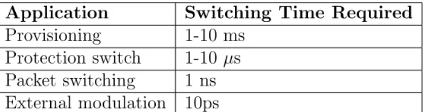
Application Switching Time Required Provisioning 1-10 ms

Protection switch 1-10 µs Packet switching 1 ns External modulation 10ps

Table 1.1: Applications for optical switches and their switching time require-ments.

1.3.4 Thermo-Optic Effect

Thermo-optic effect stems from the temperature dependence of polarizability [10]. Temperature can change the polarization directly or it may change the material density because of the thermal expansion coefficient. The polarizability also depends on the mass density. So the temperature difference creates refractive index change.The thermo-optic effect is present in all practically used waveguide materials. The most important examples of such materials are silicon, fused silica and polymers. Thermo-optic devices receive the great attention because of their low cost fabrication and polarization independent operation in low speed optical network application.

Optical modulators are used in optical networks for a variety of applications. The main important parameter in these kinds of application is switching time which varies from few milliseconds to subnanoseconds. Table 1.1 summarize the application areas of optical modulators and their switching time requirements [11]. In provisioning the modulators are used in optical crossconnects to reconfigure them to support new light paths. So for this application modulators with millisecond switching times are acceptable. Another application is protection switching. Here the modulators are used to switch the traffic stream from one fiber to another fiber in case the primary fiber fails. The required switching times is in the range of few milliseconds to hundred microseconds. Packet switching is used in high speed application. In this network in order to switch the signal on a packet the switching time must be much smaller than the packet duration. The switching time is in the order of a nanoseconds in packet switching. Finally, in order to turn on and off the data in front of a

(20)

Type Switching Time Mechanical 10 ms

Thermo-optic 1 ms Electro-optic 1 ns- 10 ps

Table 1.2: Comparison of different optical modulators with respect to their switching time.

laser source external modulation is used. In this case, the switching time must be a small fraction of the bit duration. So the external modulator must have picoseconds switching time.

1.4 Thermo-Optic Waveguide Materials

There is growing interest in the switching of light with planar optical components for applications in optical fiber telecommunications. Today, the main technology for planar modulator fabrication is Ti-diffusion in LiNbO3 [12], where the

switching is achieved using electro-optic effect. These components can be switched very fast, but are generally polarization sensitive and expensive. In some applications polarization insensitivity is more important than the switching speed. For example by-pass switching in LAN’s with ring topology and circuit switching for video distribution. For these applications optical waveguide modulators using the polarization independent thermo-optic effect can be a good alternative. And also thermo-optic control of optical modulators is attractive from viewpoint of simplicity and low cost. The most important examples of such materials are silicon and polymers.

Silicon is the most commonly used material in electronics. Its technology is highly developed so it offers a large potential for low cost optical devices. There is no inversion symmetry in Si crystal. Since the electro-optic effect (Kerr-effect) in silicon is too small [13], only the plasma dispersion effect and the thermo-optic effect are promising candidates for the realization for thermo-optical modulators. In addition to plasma dispersion effect, high thermo-optic coefficient of Si offer a good possibility for influencing the optical wave. According to Chapter 2 only

(21)

1-5K temperature difference is sufficient for refractive index change of 2×10−4_.

In addition to switching time, power consumption is also important parameter for thermo-optic devices [26]. In thermo-optic modulators power consumption depends on thermo-optic coefficient and thermal conductivity [14]. In order to decrease the operating power low thermal conductivity and high thermo-optic coefficient are needed. Polymers are good candidates for this kind of application because of their low thermal conductivity. Because of easy and low cost waveguide fabrication techniques such as spin coating at low temperature polymers have received the great attention in thermo-optic modulators fabrication.

(22)

Chapter 2 Elements of Thermo-Optic

Modulation

Modulation of optical output in Mach-Zehnder interferometer devices is obtained by modulating the optical path difference between the arms of the interferometer. In devices made of Si and polymers where the electro-optic effect is absent, this is done by modulating the temperature of the arms to invoke the temperature dependence of the refractive index. Local modulation of the refractive index is achieved by supplying a square wave electrical pulse train to an appropriately placed heater on one arm of the interferometer. Understanding heat transfer in these devices is, therefore, important. This chapter is devoted to theoretical background of thermo-optic devices. The origins of the thermo-optic effect in silicon and polymers will be given. Analytical and numerical methods for solution of heat transfer problem which will be used in next chapters will also be introduced.

2.1 Thermo-Optic Effect

The change in refractive index n, of a material at temperature T , is due to the change in density ρ, and due to the thermal change in polarizability. The rate of

(23)

CHAPTER 2. ELEMENTS OF THERMO-OPTIC MODULATION 9

change of index with temperature dn

dT can be written as [15] dn dT = ( δn δρ)T( δρ δT) + ( δn δT)ρ (2. 1) or dn dT = −(ρ δn δρ)Tγ + ( δn δT)ρ (2. 2)

where γ is the coefficient of volume expansion of the material. From the Lorentz-Lorenz (LL) equation, The following expression for (ρδn_δρ)T

(ρδn

δρ )T = (1 − Λ0)

(n2_{+ 2)(n}2_{− 1)}

6n (2. 3)

where Λ0 is the strain polarizability constant that has been introduced by

Muller [16] to take into account the effect of density changes on the atomic polarizability of the material. Temperature induced index changes for polymer and Si need to be calculated , separately.

For polymers, Λ0 is small compared to unity as a consequence of weak

interaction between the molecular units. For example, value of Λ0 is 0.15 for

polymethlylmethacrylate [17]. As the refractive index of most polymers is ∼1.55 and the thermal expansion coefficient is 2×10−4_{, the first term of the Equation}

2. 2 becomes

− (ρδn

δρ)Tγ ∼ −10

−4_/0_C. _{(2. 4)}

The thermal change of the refractive index at constant density, that is, the second term in Equation 2. 2, is small. For example for polymethlylmethacry-late [17]

− (ρδn

δT)ρ ∼ −4 × 10

−6_/0_C. _{(2. 5)}

Therefore it can be concluded that the thermo-optic coefficient in polymers has a large negative value as it is determined predominantly by density change caused by the strong thermal expansion in these materials. The value of refractive index changes becomes

(24)

CHAPTER 2. ELEMENTS OF THERMO-OPTIC MODULATION 10 dn dT ∼ −(ρ δn δρ)Tγ ∼ −10 −4_/0_C _{(2. 6)}

for glassy polymers.

For silicon, Λ0 is ∼ 0.5 and thermal expansion coefficient has a value of

2×10−6_{. The refractive index of silicon is ∼3.4 (λ =1.55µm). From Equation}

2. 3 it follows that

− (ρδn

δρ)Tγ ∼ −4/

0_C. _{(2. 7)}

Therefore the first term in Equation 2. 2 is of the order of

− (ρδn

δT)ρ∼ −10

−5_/0_C. _{(2. 8)}

and finally the thermal change of refractive index caused by density change can be estimated as dn dT ∼ −(ρ δn δρ)Tγ ∼ −10 −5_/0_C. _{(2. 9)}

On the other hand, the temperature dependent refractive index change of silicon is about 2×10−4_/0_{C. In silicon, thermo-optic effect is mainly due to the second term}

of Equation 2. 2 which originates from the thermal changes in the polarizability. It can be concluded that the thermo-optic coefficient of silicon is of the same order of magnitude with polymers and its sign is positive, and opposite to that of the coefficient in polymers. The optical modulation depends on the absolute value of refractive index changes so that its sign does not effect the modulation mechanism.

2.2 Heat Transfer in Solids

Heat transfer can be defined as the transport of energy due to a temperature difference. There are mainly three distinct mechanisms by which heat transfer takes place: (i) Conduction, (ii) Convection, (iii) Radiation. In solids, convection is absent and heat transfer via radiation can be neglected for room temperatures. Therefore, conduction is the dominant heat transfer mechanism in solids [18] under our consideration.

(25)

Heat conduction in solids is due both to the excitation of the vibrational modes of atomic molecular species and the motion of free electrons. Conduction is governed by Fourier’s law stated as; the rate of heat conduction ( ˙Q) is proportional to the area (A) normal to the direction of the heat flow and to the temperature gradient(dT

dx) in the direction of the heat flow. Thermal conductivity

defined by k and has the unit of W/mK(SI). A mathematical statement of Fourier’s law for 1D heat flow is

˙ Q = −AdT dx (2. 10) or, q = Q˙ A = − dT dx. (2. 11)

Thermal analysis concerns itself with both the steady state and transient conduction of heat. Considering the principle of conservation of energy for volume element, the general heat transfer equation can be written as

∇2_{T +} ˙q k = ( ρC k ) ∂T ∂t. (2. 12)

Where C is the heat capacity. For steady state condition without internal heat generation equation becomes;

∇2_{T = 0} _{(2. 13)}

and transient heat equation without internal heat generation takes the following form

∇2_{T = (}ρC

k ) ∂T

∂t. (2. 14)

Initial conditions for the differential equations specify the temperature distri-bution throughout the entire region at time, t = 0. Boundary conditions can be formulated in three different types as; first, second and third kinds. A first kind boundary condition defines the temperature on the boundary explicitly, for example T(0,t)=10 0_{C. A second kind of boundary condition defines the}

temperature on the boundary implicitly, in terms of heat flux. For example

q(L, t) = (dT

dx)x=L = − 100

(26)

where k is the thermal conductivity of the material. A boundary condition of third kind specifies the temperature gradient at the surface in terms of an external heat transfer coefficient h, the surface temperature Ts and the reference temperature

Tref, for example,

− k(dT

dx)x=0 = h(Ts− Tref). (2. 16) In thermo-optic devices, periodic boundary conditions are created by electrical heating. So, the time dependent solution of heat equation with periodic boundary conditions takes primary importance.

We seek solutions of the type

T = uei(wt−ε) _{(2. 17)}

substituting in the differential equation, it follows that u must satisfy d2_u

dx2 =

iw

k u (2. 18)

so the solution of period 2π

w should be in the following form

T = Ae−kxcos(wt − ε − kx) (2. 19) when the surface temperature is a periodic function of time of period 2π

w, we can

obtain the solution by using the Fourier series for θ(t)

θ(t) = A0+ A1cos(wt − ²1) + A2cos(2wt − ²2) + ... (2. 20)

and if the θ(t) is the square wave with the period τ then we find the temperature [19]. T = 4 π X ₁ (2n + 1)e −x√(2n+1)π/2kτ_sin[(2n + 1)πt τ − x{ (2n + 1)π 2kτ } 1 2] (2. 21)

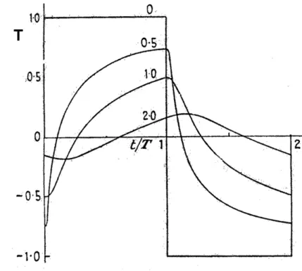
In Figure 2. 1 temperature is plotted as a function of time in which the higher harmonics disappear and square wave gradually becomes exponential and then sinusoidal as the thermal conductivity decreases and heat capacity increases. In

(27)

Figure 2. 1: Oscillations of temperature caused by periodic boundary conditions in a material with different thermal properties.

Figure 2. 1 each axis normalized and each curve represents the temperature response of different materials with different thermal properties .

Finally, the analogy between the theory of alternating current circuits can be noted. ρc k ∂V ∂t = − ∂2_V ∂2_x (2. 22) I = −kΩ∂V ∂x (2. 23)

where V is potential, k is the electrical conductivity and c is the capacitance. The temperature is equivalent to potential and heat flow can be represented by current in circuit theory. The theory of electrical circuits is well known. This implies that the behavior of a complicated thermal network may be modelled by the analogy with circuit theory.

(28)

2.3 FEM Simulation of Heat Transfer in

Thermo-Optic Devices

There are many engineering problems for which the exact solution for heat transfer equations can not be analytically obtained. This difficulty requires the use of numerical methods and approximations to deal with such problems. There are two common classes of numerical methods for solution of differential equations: (1) Finite difference methods, (2) Finite element methods. We have made use of the finite element method to analyze the thermal effects in optical devices. The finite element method is a numerical procedure to obtain a solution to variety of problems such as steady state and transient problems in stress analysis, heat transfer and electromagnetism. The significant step in utilization of finite element method was taken by Boeing in 1950’s to model airplane wings [20]. Galerkin’s method is one of the most commonly used procedures in finite element formulation. The Galerkin’s method requires the error (<) to be orthogonal to the same weighting functions φi, which known as shape functions,

according to the integral [20].

Z

φi<dy = 0 (f or i = 1, 2, ..., N ) (2. 24)

In this representation it is needed to determine the shape function according to a defined element. The first approximation is dividing the solution domain into elements. Next step, is to choose the element type and determine the shape functions. Applying the Galerkin method, the approximate solution can be found for each element, then assembly of elements leads to the global conductance matrix. By applying the boundary conditions, nodal temperature solution can be found from the final sets of linear equations.

ANSYS and FEMLAB are commercial computer programs that allow to model the physical problem with finite element analysis. FEMLAB has a powerful, interactive environment for modelling and solving scientific and engineering problems based on partial differential equations. Figure 2. 2 represents the solving procedure of FEMLAB. Drawing the geometry under

(29)

consideration is the first step, in which the device geometry is defined Fig 2.2.a. Second step is meshing the area, Fig2.2.b. Through the meshing process, partial differential equation can be solved for each element as explained earlier, Fig2.2.c. After drawing and meshing steps, the required material properties and boundary conditions are defined. Finally, by running the numerical solver, the solution is obtained.

The accuracy of the solution depends on the element type and meshing size. We can improve the accuracy of finite element findings by either increasing the number of linear elements used in the analysis or using a higher order interpolation function. In linear function, two nodes are enough to define the temperature distribution through the element. For example, for 1-D linear element,

Te _{= c}

1+ c2X (2. 25)

For 1-D quadratic element, the defined temperature distribution is

Te _{= c}

1+ c2X + c3X2. (2. 26)

Utilizing a quadratic function instead of a linear function requires that we use three nodes to define the computational element. This higher order interpolation increases the accuracy of the solution but also increases the required computational time unacceptably.

(30)

(31)

Chapter 3 Thermo-Optic Multi-Mode

Interference Modulators

In this chapter, conditions for single mode waveguide design is elaborated and theoretical background of multi-mode interference (MMI) couplers is presented. In addition to MMI coupler based thermo-optic devices design, finite element simulations of heat diffusion is discussed.

3.1 Design of Single Mode Waveguides

The design of single mode waveguides starts with the design of a slab waveguide using materials of choice as the device platform. The slab waveguides are easy to design because of their simple geometry and well defined boundary conditions. However, slab waveguides cannot confine the light in the lateral direction. For integrated optical applications, it is required to guide the light in a predefined optical path. In order to achieve vertical and lateral confinement of light dielectric rectangular waveguides are most commonly used in integrated optics.

Three possible configurations for rectangular waveguides are shown in Figure 3. 1. Analysis of this kind of waveguides is difficult because it is impossible to simultaneously satisfy all boundary condition with any analytical expression.

There are two frequently used waveguide design tools, namely effective index

(32)

CHAPTER 3. THERMO-OPTIC MULTI-MODE INTERFERENCE MODULATORS 18

Figure 3. 1: Different types of optical waveguides

(33)

method (EIM), which is an relatively easy method useful for most of the design purposes and the beam propagation method (BPM), which is a numerical simulation technique based on finite difference solution techniques. The effective index method convert the two dimensional problem into one dimensional problem. In this method the rib waveguide is divided into three slab structures for each of which the exact solution is straightforward. The propagation constant, β for guiding mode is calculated from the eigenmode equations of the slab waveguide for two slab waveguide structures. Then effective index is calculated for each structure using,

nef f =

β κ0

. (3. 1)

Using the effective indices an artificial slab waveguide structure is formed as in Figure 3. 2 and calculation of the β is repeated for this structure using Equation 3. 1. The resulting effective index is the effective index of original rib waveguide. Finally, the single mode condition for final slab waveguide can be stated as

t < c + √ r 1 − r2 (3. 2) where c = 0.5 t = wef f Hef f r = hef f Hef f hef f = h + q Hef f = H + q wef f = w + 2γuc kqn2 f − n2uc q = γuc kqn2 f − n2uc + γlc kqn2 f − n2lc (3. 3)

and nf,nuc,nlc are the refractive indices of the guiding region, upper and

lower cladding, respectively. After initial design using the EIM, the result can be verified by using BPM simulation by calculating the mode spectrum of the waveguide.

(34)

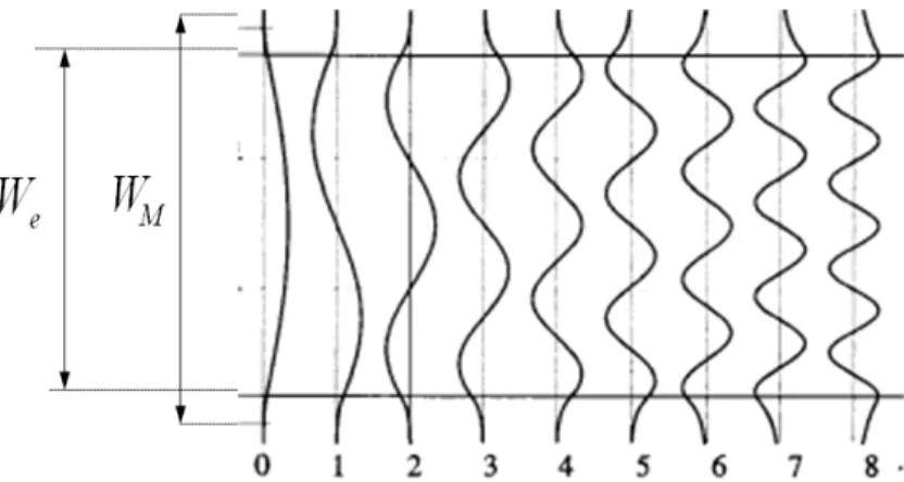
Figure 3. 3: Schematic diagram of MMI coupler.

3.2 Optical Multi-Mode Interference Couplers

In general, a MMI is a multimode waveguide that is fed by single mode waveguide(s) and allows the interference of waves diffracting at the input port(s) leading to nodes (constructive interference) and antionodes (destructive interference) at which ouput port(s) may be placed. The operation of Multi-Mode Interference (MMI) devices is based on the self-imaging principle. This principle can be stated as the property of a multi-mode waveguide by which an input field profile is reproduced in multiple images at periodic intervals along the propagation direction [21]. Figure 3. 3 illustrates the basic structure of an MMI coupler. It consists of a multi-mode waveguide and with a single mode input waveguide and two single mode output waveguides. Single mode waveguides are designed to launch or recover the light and multi-mode waveguide is designed to support a large number of modes for general interference for self imaging. In Figure 3. 3 an MMI coupler designed to split light into two output channels is illustrated. Ψ0 is being an input field profile, and after sudden transition

multi-mode region, Ψ0 spreads into all available modes of the multimode waveguide.

Typically, multi-mode waveguides are chosen to support more than 3 modes. Using the orthogonality relation we can write the field profile as

Ψ(y, z) =Xcνψν(y) exp[j(wt − βνz)] (3. 4)

(35)

Figure 3. 4: Example of amplitude normalized lateral field profiles corresponding to step-index multi-mode waveguide.

cν =

R

Ψ(y, 0)ψν(y) d(y)

qR

ψ2

νdy

. (3. 5)

For mode propagation analysis, modes of the waveguides should be determined. For a multi-mode waveguide of width WM, ridge refractive index nr and cladding

refractive index nr, and wavelength λ0, the dispersion equation for the lateral

modes can be written as

k_yν2 + β_ν2 = k₀2n2_r (3. 6) for which k2

yν is defined as the lateral wave number for mode ν

k0 = 2π λ0 (3. 7) kyν = (ν + 1)π Weν (3. 8) and the propagation constants spacing can be written as

(β0− βν) = ν(ν + 2)π 3Lπ . (3. 9) Lπ = π (β0− βν) = 4nrW 2 e 3λ0 (3. 10)

(36)

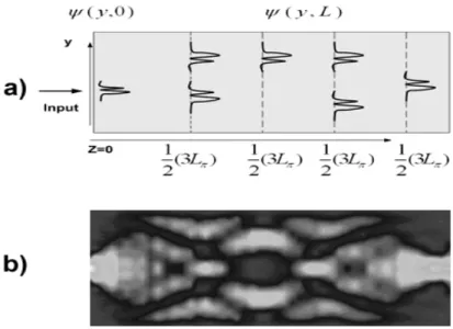
Figure 3. 5: a)Multi-mode waveguide showing the input field, mirrored single image, a direct single image, and two fold images. b)BPM simulation of multi-mode waveguide to illustrate the image formation.

Taking the fundamental mode as a common factor out of the sum, the field profile becomes

Ψ(y, z) =Xcνψν(y) exp[j(β0− βν)z]. (3. 11)

Figure 3. 6 shows a step index multi mode waveguide of width We and refractive

index nr. It will be seen that under certain circumstances Ψ(y, L) will be a self

imaging of input field Ψ(y, 0) with an analytical relation of

Ψ(y, L) =Xcνψν(y) exp[j(

ν(ν + 2)π 3Lπ

)L]. (3. 12) It can be shown that

exp jν(ν + 2)πL 3Lπ

= 1 (3. 13)

ÃL = p(3Lπ) with p = 0, 1, 2, ... Ψ(y, L) will be the single image of Ψ(y, 0)

Ψ(y, p(3Lπ)) =

X

cνψν(y) = Ψ(y, 0) (3. 14)

(37)

ÃL = (p₂)(3Lπ) with p = 1, 3, 5, ... Ψ(y, L) will be the multiple image of Ψ(y, 0)

Ψ(y, (p 2)(3Lπ)) = ( 1 + (−j)p 2 )Ψ(y, 0) + ( 1 − (−j)p 2 )Ψ(−y, 0) (3. 15) Similarly, the length at which multiple images form can be determined to be between the direct and mirrored image lengths. The N fold images are formed at

L = p

N(3Lπ) (3. 16)

Other results appear when restrictions on excitation of the modes come into picture. Restricted excitation allows to design even smaller devices but also has lower tolerances to fabrication parameter variances. In this case, this restricted interference is of two types: paired and symmetric interference. In paired interference, there is selective excitation. If the input beams are launched at symmetric input channels at y=±We/6 , the overlap integral will vanish

for antisymmetric modes. Therefore cν=0 for ν=2,5,8,... When the selective

excitation is fulfilled the modes contributing to imaging are paired, i.e. the mode pairs 0-1, 3-4, 6-7, ... have similar relative properties, for example each even mode leads its odd partner by a phase difference of π/2 at z=Lπ/2. This mechanism is therefore called paired interference. In symmetric interference case, upon which only 1xN MMI splitters can be designed, only even modes are excited.

mod4[ν(ν + 2)] = 0 f or ν even (3. 17)

It is clear that the length periodicity of the mode phase is reduced four times if

cν = 0 f or1, 3, 5, ... (3. 18)

This condition can be achieved by center-feeding the multi mode waveguide with symmetric field profile. The imaging is obtained by linear combinations of the even symmetric modes and the mechanism is called symmetric interference. N fold imaging occurs at even shorter distances, formulated with

L = p N(

3

(38)

The length of the MMI coupler depends on the width of the multimode waveguide. First of all, it is required to determine the distance between the input ports for sufficient optical insulation between them. Taking this into account, the width the MMI is determined and finally the length of the coupler is calculated from Equation 3. 19. The design is finally confirmed by BPM code.

3.3 Multi-Mode Interference Modulator

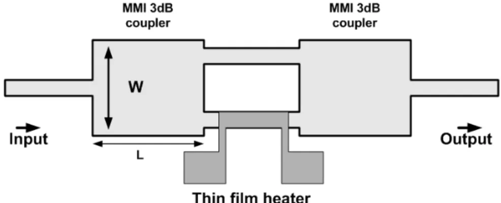
Intensity modulation of guided light is one of the most elementary operation in integrated optics. Intensity modulation can be divided into distinct classes such as absorption, radiation and interference based intensity modulation. Example of interference based modulators is Mach-Zehnder interferometers [22]. Mach-Zehnder interferometer (MZI) has been extensively used in realization of optical processing, because of the small device dimensions, excellent tolerance to polarization and wavelength variations, acceptable fabrication tolerance, low excess losses and ability to split light into any number of ports offer superior performance for optoelectronic applications. Figure 3. 6 illustrates the basic structure of an MMI modulator where the input signal is split by a 3-dB MMI coupler and fed into phase shifters and is recombined by another MMI coupler. A MMI based Mach-Zehnder interferometer is limited by power imbalance that may be present at the output of the splitter stage and the output combiner stage. Because of the good balancing MMI based modulators are ideal building blocks for Mach-Zehnder structures [25].

The MZI configuration allows one to change light intensity in the output channel by introducing a phase difference between the two input arms of the second MMI. In the thermo-optic devices, this phase difference is achieved by heating one arm, resulting in a temperature difference between the arms. At the output port, the images of incoming waves interfere. If E1 and E2 are the electric

field profiles of the incoming waves with φ phase shift between them

E1 =

E0

(39)

Figure 3. 6: Schematic diagram of MMI modulator.

E2 =

E0

2 cos(wt + φ) (3. 21)

at output port as a result of the interference of two images of incoming waves, we can write the new electric field and power as

ET = E0 2 cos(wt + φ) + E0 2 cos(wt) (3. 22) I = hE_T2i = E₀2cos2(φ 2) = I 2 0cos2( φ 2). (3. 23) The phase shift can be written in terms of index difference and finally, it is possible to calculate the output intensity as a function of temperature difference

I = cos2₍∆φ

2 )) = cos

2₍πχ∆T Lh

λ ) (3. 24)

where ∆T is the temperature difference between the two waveguide cores of the phase shifter arms, χ is thermo-optic coefficient of the core material, λ is the free space wavelength, and Lh represents the length of the heater. For our

devices on Si Lh=1mm, λ = 1.55µm and χ of 2×10−4/0C, a phase difference of

π is achieved with a temperature difference ∆T =3.75 0_C.

Several analytical analysis methods of the MMI coupler based modulators are available [27]. After designing the MMI couplers and cascading them to form the Mach-Zehnder interferometer, we have made use of a mode propagation method

(40)

Figure 3. 7: BPM simulation of MMI modulator for off (a) and on state (b).

(BPM) based on effective index (2D) approximation to fine tune the dimensions and confirm the operation of MMI based Mach-Zehnder switch as was explained in reference [21]. Figure 3. 7a shows the BPM simulation of field distribution on MMI modulator where there is a π phase shift between two arms in MZI section and output light intensity is zero and in figure 3. 7b there is no phase shift, intensity of the output light is maximum.

Device Design

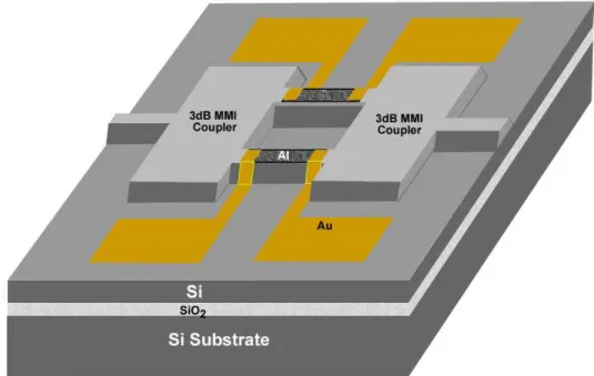
We have chosen Bond and Etch Back (BESOI) material with SiO2 layer thickness

1µm to create a sufficient optical insulation between the core silicon and the silicon substrate. A schematic illustration of the MMI based MZ modulator is shown in Figure 3. 8. The trench between the waveguides prevents the heat cross flow to create high temperature difference between the phase shifter arms at lower electrical power. The SiO2 buffer layer between the optical waveguides

and evaporated Al heater on the top are required to prevent optical loss. The length of the heater is 1 mm. The distance between single mode waveguides is

(41)

Figure 3. 8: Sidewiev of MMI modulator

chosen as, 12µm for sufficient optical and thermal insulation. Width of the MMI is chosen as 30µm. Then length of MMI coupler is calculated to be L, 1100µm, using Equation 3. 19.

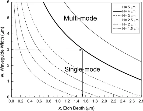
In order to increase the modulation depth of the switch, single mode condition is required in phase shifter region to prevent different phase accumulation for different modes under the same index change. The exact mode analysis of SOI waveguide is a bit cumbersome and exact analytical solution is difficult to find. Instead we use the approximations described in Section 2.1, namely beam propagation method (BPM) and effective index method (EIM). After an initial design using the EIM, the results were verified with BPM. Single mode condition for SOI waveguides was calculated by making use of the effective index method, the results of which are generalized and plotted in Figure3. 9. Once the top Si layer thickness acting as the core is selected, the area under the corresponding curve in Fig 3.9 define the single mode region and the remaining areas are multi-mode. Thus, it is possible to choose a variety of combinations for waveguide width, w, and the etch depth needed to obtain the required rib height. The

(42)

Figure 3. 9: Single mode condition for different Si top layer thicknesses. For H=4 um, waveguide width of 3 um requires the etch depth to obtain the rib as 1.4 um

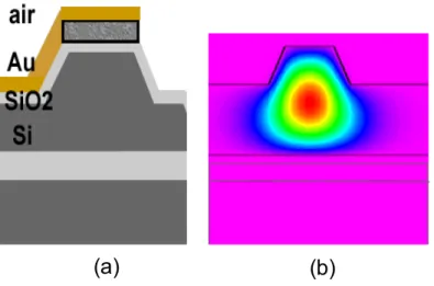
mode spectrum and shape of the waveguide were both verified by using BPM which solves the scalar or vector wave equation for any structure defined by n=n(x,y,z). The cross section of the single mode waveguide and the mode shape of the TE fundamental mode as obtained by BPM are depicted in Figure 3. 10. Based on these results, a structure for A single mode SOI waveguide was determined with the following parameters; Bottom cladding thickness tbc=1 µm,

upper cladding thickness tuc = 0.2µm, slab waveguide thickness hslab = 2.6µm,

rib height hrib = 1.4µm and rib width wrib= 3µm.

In order to understand the working principles of the thermo-optic switch, a thermal analysis of the device was performed using Finite Element Method (FEM). By doing the thermal analysis, switching power calculation and frequency response of MMI based Mach-Zehnder modulator was obtained using FEMLAB

(43)

Figure 3. 10: (a)Schematic diagram of waveguide structure, (b) TE fundamental mode shape for Si ridge waveguide as calculated by BPM.

software. FEM was used to perform both linear stationary and time dependent thermal analysis of MMI based Mach-Zehnder modulator. Heat transfer involved in these devices is governed by the heat equation

ρC∂T

∂t − ∇.(k∇T ) = Q (3. 25)

where ρ is the density, C is the heat capacity, k is the isotropic thermal conductivity and Q is the external heat input. In our simulations Q is the heat input provided by the metal heater. We define heat input as heat per unit volume (W/µm3_{) and in time dependent simulations we apply a square wave heat pulse}

to the metal electrode and calculate the temperature response. The material properties used in all the simulations for Si and SiO2 can be listed as ρSi =

2330kg/m3_{, C}

Si = 703J/kgK, kSi = 163W/mK ρSiO2 = 2220kg/m

3_{, C}

SiO2 =

745J/kgK, kSiO2 = 1.38W/mK [32].

Figure 3. 11 shows the simulated two dimensional steady state temperature distribution at the phase shifter region of the MZI. The heater is placed on the left single mode waveguide separated by a trench from the parallel single mode waveguide on the right without a heater. It is observed from the figure, that the power created at the metal heater results in the heat flow into the silicon layer. Surprisingly, the air above the electrodes also heat up but due to the low thermal

(44)

Figure 3. 11: 2D steady state temperature distribution of the MMI modulator. The power applied to the electrode is 114 mW,

conductivity of air, temperature increase is small and consumes only negligible heating power. Temperature distribution at guiding area is uniform. The trench between waveguide arms prevents the heat flow to the alternate waveguide to the left and so creates sufficient temperature difference between them. SiO2 layer

underneath the core layer also effects the heat diffusion, and because of its low thermal conductivity heat diffuses laterally in the silicon layer away from the device rather than into the silicon substrate.

In this simulation, we keep the bottom layer at constant temperature (T=20

0_{C ) and zero heat inward flux is assumed at the side walls as boundary conditions.}

From Equation 3. 24, the temperature difference for zero optical output intensity is calculated to be ∆T =3.75 0_{C. This is consistent with the simulations using}

FEMLAB. The trench between the two phase shifter waveguides provides thermal insulation and prevents heating of the parallel second waveguide, allowing for lower switching power and faster response. To obtain the switching power using FEM simulations, we calculated the required heat input from the thin metal film electrode with appropriate boundary conditions. Total switching power Pπ was

(45)

Figure 3. 12: Simulation results of pulse response when 1 kHz square wave is applied to electrode. (a)applied power (b)temperature response (c)output light intensity.

calculated to be 114 mW.

Transient response of the device can also be simulated using FEMLAB software. In this simulation, thermal response and the ensuing optical response of the device to an applied electrical square pulse is calculated. The rise and

(46)

Figure 3. 13: Simulation result for modulation depth of output light intensity as a function of frequency.

falls times of the optical pulses at the output of the device may be limited by thermal and electrical considerations. The amplitude modulation of thermo-optic devices is restricted by thermal rise and fall times. Rise and fall times depend on the thermal properties of the material as discussed in Chapter 2. Heat capacity C and thermal conductivity k determine the temperature rise and fall time. In Fig 3.12, we observe the applied electrical power 114 mW at 1 kHz, the corresponding temperature rise in the waveguide core and the resulting optical intensity response at the output port. It should be noted that the temperature rise upon the application of the electrical pulse is very fast but the temperature fall upon the termination of the electrical pulse is slow and follows an exponential like decrease. This indicates that the frequency response of the devices are limited at the cooling stage as opposed to the heating stage. This is due to the relatively thick SiO2 layer used under the core layer to optically isolate the core layer.

It should be noted that SiO2 thickness greater than 0.25 µm is sufficient for

optical isolation and may decrease the cooling time further. Many simulations at different frequencies were made. A summary of these simulations are plotted in Figure 3. 13. As the frequency of the applied electrical pulse is increased the

(47)

Silane (2% SiH4) Flow Rate) 180 sccm

NH3 Flow Rate 45 sccm

Process Pressure 1000 mTorr

RF Power 10W

Substrate Temperature 250 0_C

Table 3.1: PECVD process parameters for Si3N4 growth.

required temperature difference between waveguides cannot be achieved because waveguide cannot be cooled as fast as the applied electrical power. Therefore, the modulation depth of the output intensity will decrease. The 3-dB cutoff frequency can be observed from figure 3. 13. Modulation depth is within 50% of its maximum value at 50 kHz when a the switching power of 114 mW is applied.

Device Fabrication

We start the fabrication process by cleaving a SOI chip with dimensions of 10×20 mm2 _{from the wafer. SOI based waveguide devices are typically formed on}

the top silicon layer. In order to etch the silicon, pattern transfer is done by using specific solutions resulting in etching of the uncoated regions. Potassium hydroxide (KOH) solution is one of the anisotropic wet etchants of Si [30]. In conventional lithography process UV light sensitive photoresist (PR) is used for pattern transfer. However, PR cannot withstand to KOH solution and as such PR cannot be used as a mask to etch Si. So silicon nitride (Si3N4) film is required

to use as a hard mask for pattern transfer. For this purpose the chip is degreased in a three solvent cleaning process prior to covering its top surface with a layer of Si3N4. After sample cleaning and drying the chip at 1200C for 60 sec , the sample

is coated with Si3N4 by plasma enhanced chemical vapor deposition (PECVD)

technique. A fully automated planar plasma reactor have been used (Plasmalab 8510C). The growth rate depends on the process parameters. The recipe file which results in a growth rate of 100 A0 _{/min Si}

3N4 is given in Table 3.1.

The cleaned sample is placed on the lower electrode plate of the PECVD unit which is heated before the process starts. After 2000 A0_{of Si}

(48)

Figure 3. 14: All Patterning steps of SOI optical waveguides, (a)SOI structure, (b)Si3N4 Deposition, (c)Photoresist Spinning, (d)Photolithography,

(e)HF Etching, (f)KOH Etching, (g)Removing Si3N4

pattern transfer is accomplished by conventional optical lithography. Surface of the sample is coated with AZ5214 photoresist by spinning at 5000 rpm for 40 sec. The uniformly PR coated sample is dried on a hot plate at 120 0_{C for 50 seconds}

(49)

This results in a layer of photoresist with thickness of 1.4 µm. Then the mask is aligned in the mask aligner (Karl Suss MJB-3 HB/200W). After exposing with UV lamp, the sample is developed in AZ400K developer solution to remove the exposed material. PR pattern is transferred to the Si3N4 layer. by etching Si3N4

in a dilute HF solution. In this process PR behaves as the masking material. In order to increase the hardness of PR baking at 1200_{C is used before etching in}

dilute HF solution. The HF solution is a mixture of 1:1000 HF:H2O and has a

etch rate of 34 A/s. The PR is then removed by acetone (ACE). Finally, the sample is ready for etching in a KOH solution using Si3N4 as the etch mask.

It is important to note that for low loss waveguides minimum surface roughness of the waveguide walls is required. Due to the anisotropic etching properties of KOH solution, KOH solution parameters such as concentration and temperature need to be optimized. As a result, a solution of 1:3:1, KOH:H2O:ISO

at 40 0_{C is chosen as optimum parameters. The etch rate of this solution is 470} 0_{A/min. The etch depth for a single mode rib waveguide requires that the silicon}

layer be etched approximately 1.4µm. Therefore, etching the ribs with KOH solution takes 30 minutes. After KOH etching, the Si3N4 mask is removed by

the same HF solution used earlier. Figure 3. 14 illustrates the fabrication steps for waveguide patterning. After the etching the waveguide pattern, second step is to define the trench between the waveguides. Trench is etched in silicon with standard optical lithography process used earlier. Si3N4 is used as a hard mask

again. First, the sample is coated with Si3N4and then using PR and conventional

photolithography the trench pattern is transferred to the PR. The second step is to transfer the PR pattern onto Si3N4 layer by using dilute HF. Figure 3. 15

illustrates the trench patterning steps. Then PR is removed and then using KOH solution, trench is etched in silicon. Finally, Si3N4 mask is removed with dilute

HF solution. Care must be taken at this step to assure best alignment possible of the trench with the waveguides, since the device is relatively long.

The next fabrication step is PECVD SiO2 deposition for top cladding layer.

There are three requirements for this deposition: Firstly, the thickness of the layer should be large enough for optical insulation between guided light and metal

(50)

Figure 3. 15: Trench patterning steps of SOI optical waveguides (a) Si MMI waveguide, (b) Si3N4 Deposition, (c) Defining trench pattern, (d) KOH Etching,

(e) Removing Si3N4, (f) SEM photograph of MMI modulator .

Silane (2% SiH4) Flow Rate) 180 sccm

N2O Flow Rate 25 sccm

Process Pressure 1000 mTorr

RF Power 10W

Temperature 250 0_C

Table 3.2: Process Parameters for SiO2.

heater. On the contrary, the second requirement is that the SiO2 be thin for

good heat transfer. By using BPM simulation the calculated minimum thickness for optical isolation is found to be 0.25 µm. Finally, the optical quality of the oxide layer should be sufficient for minimizing the optical loss. SiO2 is grown by

PECVD with the process parameters listed in table 3.2. This recipe results in a layer of SiO2 with refractive index of 1.473.

5 mµ

µ µ

(51)

Figure 3. 16: Electrode metallization of thin film heaters (a) Patterned Si waveguide, (b) Spinning PR, (c) Defining heater, (d) Al evaporation, (e) Liftoff, (f) Top view optical microscope photograph of heaters and electrodes.

The final step is patterning the metal heater. The thin film electrodes were formed by conventional lift-off process. Aluminum is suitable material as a metal heater because of its adhesive properties on SiO2 surface and its low electrical

resistance. First, electrode patterns were defined by photoresist and then Al was evaporated on the sample. Then, by rinsing in ACE the photoresist and the Al on it was removed. Figure 3. 16 illustrates this process. The thickness of the Al film is very important parameter in order to reach acceptable heater resistance. Evaporation is more suitable for low resistive metal deposition. Grain formation in metal film during sputtering increases the resistance dramatically. For a heater with a resistance of 50 Ω we deposited 0.2µm thick 1 mm long and 3 µm wide Al electrode using standard thermal evaporation process. Final devices require that waveguide facets be of very good quality. This can be obtained with a cleaving

(52)

process. It was found that thinner substrates produce better facets upon cleaving. Therefore, finished devices were covered with PR and glued on a Si wafer for back side etching. A KOH solution at 50 0_{C for 40 hours is used to thin down the}

substrate to approximately 200 um. After cleaning the device, a Si cleaving pen is applied from the back side to cleave the devices at the desired location.

Results

Figure 3. 17 shows our optical measurement setup. 1.55µm DFB laser (LDM-7980) is coupled to cleaved facets with a single mode fiber. In this setup, light is coupled into the waveguide by bringing the fiber carrying the light in close proximity to the waveguide facet. This butt-coupling technique requires optically cleaved facets for the devices. For TE and TM measurement polarization of the laser was controlled via a polarization controller and checked by a polarizer at the output. A field microscope is used to align the fiber with the end facets of the waveguide. The light exiting the device may be collected by a microscope objective or by another single mode fiber, both of which are available on the setup. The light is then detected either by a photodiode detector or by an IR camera (Electrophysics Microviewer 7290A) with the help of a focusing lens. Both Ge and InGaAs photodiodes (Thorlabs DET410) have been used. The photodiode output is monitored by powermeter for d.c. measurements or by an oscilloscope (HP 54603B) for a.c. measurements. The DFB laser used in this work lases at 1.55 µm which can be tuned by controlling the temperature of the device. For modulation purposes, external electrical signals are applied by using probes with fine tips touching the aluminum pads on the devices. The probes are fed by a signal generator (HP 8116A) that can provide square wave pulses up to 50 MHz with amplitudes of up to 15 V.

Figure 3. 18 shows the fundamental TE mode of the MMI Modulator in the ON state as seen on the IR camera. TM mode behaves similarly after maximizing the output light intensity by fine tuning fiber position at the input waveguide and collection optics with the help of the IR camera, collected signal is routed onto the photodiode. Since the devices were designed to be normally ON, it was not

(53)

Figure 3. 17: Optical measurement setup.

Figure 3. 18: View of T E0 mode as captured with IR camera.

difficult to find the output light. At this point insertion loss of the devices were measured. Insertion loss includes all the losses that occur when the devices is inserted between the fiber and the collection optics and includes coupling losses due to differing fiber size and waveguide cross section, propagation loss through

(54)

Figure 3. 19: Normalized output light intensity as function of applied electrical power.

Figure 3. 20: Measured normalized pulse response when a square-wave voltage pulse with a 1KHz was applied.

the device, and Fresnel reflection at the input and output facets. The fiber core size of the single mode fibers is 9 µm in diameter, it is expected that there will be a large coupling loss for these devices. Furthermore, propagation losses

(55)

for MMI based devices are known to be relatively large and modulation of the light output further increases this. Finally, Fresnel reflection is due to inherent reflection coefficient of the Si facets and may be considered to be relatively large compared to fibers related loss due to large index contrast of the waveguides under measurement. The insertion losses may be reduced by using the well known techniques of appropriate tapering at the input and output of the devices, and by antireflection coating the waveguide facets.

To determine the turn off power (Pπ), the ramp voltage was applied to one of

the heater and output intensity was recorded for both TE and TM polarizations. According to Figure 3. 19 the measured switching power is approximately 120 mW for both TE and TM. As seen from the Figure 3. 19 output light intensity is minimum when 120 mW power is applied. This result agrees well with our calculated power Pπ with FEM simulations which was found to be 114 mW. We

suspect that 6 mW power difference between the calculated and the observed values stems from the longitudinal heat diffusion. To reduce computing time and satisfy stringent memory requirements, our simulations were done in two dimensions which cannot account for longitudinal heat loss along the waveguide. For time dependent response measurements a square wave voltage signal was applied to the heater. Figure 3. 20.b shows the modulated output signal, where 1 kHz signal was applied 3. 20.a. This measurement was repeated for many frequencies the results of which are plotted in Figure 3. 21. At higher frequencies, due to low thermal rise and fall times, modulation amplitude decreases. Figure 3. 13 shows that for our MMI modulator at 60 kHz the amplitude modulation falls within 50% of its maximum value 3-dB cutoff frequency is 60 kHz. This result also agrees as a representative example, Figure 3. 13 reasonably well with our FEM simulation which is shown in Figure 3. 21. The small difference between simulation and experiment stems from the difference of the material properties used in the simulation.

(56)

(57)

Chapter 4 Thermo-Optic Y-Junction

Mach-Zehnder Modulators

In this chapter, Y-junction based Mach-Zehnder interferometer is investigated. Both silicon based and polymer based devices were fabricated and their characteristics measured.

4.1 Y-junction Coupler

Mach-Zehnder interferometer (MZI) is the most commonly used optical device for coherent light modulation [22]. The principle of MZI is to split light into two different paths and then to recombine them at the output port. This splitting and recombination of guided waves can be achieved by different types of couplers such as Y-junction and multi-mode interference couplers. In this chapter, we will discuss the Y-junction 3-dB couplers and Mach-Zehnder modulators based on them. Figure 4. 1 illustrates the basic structure of Y-junction coupler.

Power splitting in Y-junction coupler is achieved by adiabatic transition from a single mode waveguide to two single mode waveguides. Figure 4. 2 represents the adiabatic transition in a Y-junction coupler. The input channel and two output channels of the coupler are all single mode. Incoming wave can only excite the first optical mode in both channels, and field profile is conserved but

Polarization independent thermo-optic modulators for integrated optics

POLARIZATION INDEPENDENT

THERMO-OPTIC MODULATORS FOR

INTEGRATED OPTICS

By

A¸skın Kocaba¸s

September 2003

Abstract

POLARIZATION INDEPENDENT THERMO-OPTIC

MODULATORS FOR INTEGRATED OPTICS

A¸skın Kocaba¸s

M. S. in Physics

Supervisor: Prof. Atilla Aydınlı

September 2003

¨

Ozet

T ¨

UMLES¸˙IK OPT˙IK UYGULAMALARI ˙IC

¸ ˙IN KUTUPSAL

OLMAYAN ISIL OPT˙IK K˙IPLEY˙IC˙ILER

A¸skın Kocaba¸s

Fizik Y¨uksek Lisans

Tez Y¨oneticisi: Prof. Atilla Aydınlı

Eyl¨ul 2003

Acknowledgement

Contents

List of Figures

List of Tables

Chapter 1

Introduction

1.1

Electroabsorption Modulators

1.2

Coupled Waveguide Modulators

1.3

Interferometric Modulators

1.3.1

Electro-Optic Effect

1.3.2

Acousto-Optic Effect

1.3.3

Free Carrier Injection Effect

1.3.4

Thermo-Optic Effect

1.4

Thermo-Optic Waveguide Materials

Chapter 2

Elements of Thermo-Optic

Modulation

2.1

Thermo-Optic Effect

2.2

Heat Transfer in Solids

2.3

FEM Simulation of Heat Transfer in

Thermo-Optic Devices

Chapter 3

Thermo-Optic Multi-Mode

Interference Modulators

3.1

Design of Single Mode Waveguides

3.2

Optical Multi-Mode Interference Couplers

3.3

Multi-Mode Interference Modulator

Chapter 4

Thermo-Optic Y-Junction

Mach-Zehnder Modulators

4.1

Y-junction Coupler