The position of countries in global value chains

(1)

THE POSITION OF COUNTRIES IN GLOBAL VALUE CHAINS

A Master’s Thesis

by

O ˘GUZHAN ERDO ˘GAN

Department of Economics ˙Ihsan Do˘gramacı Bilkent University

Ankara July 2019

(2)

(3)

(4)

The Graduate School of Economics and Social Sciences of

˙Ihsan Do˘gramacı Bilkent University

by

O ˘GUZHAN ERDO ˘GAN

In Partial Fulfillment of the Requirements for the Degree of MASTER OF ARTS IN ECONOMICS

THE DEPARTMENT OF ECONOMICS ˙IHSAN DO ˘GRAMACI B˙ILKENT UNIVERSITY

ANKARA July 2019

(5)

I certify that I have read this thesis and have found that it is fully adequate, in scope and in quality, as a thesis for the degree of Master of Arts in Economics.

———————————

Assist. Prof. Dr. Fitnat Banu Pakel Supervisor

———————————

Assist. Prof. Dr. ¸Saziye Pelin Akyol Examining Committee Member

———————————

Assist. Prof. Dr. Seda Köymen Özer Examining Committee Member

Approval of the Graduate School of Economics and Social Sciences ———————————

Prof. Dr. Halime Demirkan Director

(6)

ABSTRACT

Erdo˘gan, O˘guzhan M.A., Department of Economics

Supervisor: Assist. Prof. Dr. Fitnat Banu Pakel

July 2019

To detect the position of countries in global value chains in a consistent manner, we propose that export and import upstreamness measures of a country should be vary-ing across its trade partners over time. To formalize our argument, we define the no-tion of bilateral upstreamness between any pair of countries and show how its mea-sure is affected from country-specific factors. Moreover, we incorporate the variables in gravity literature into our estimation equations to account for how the geographi-cal factors can have an impact on their bilateral production line position. Following Antrás et al. (2012), we also consider the hypotheses tested in their paper with our more aggregated and recent data set. Similar to their results, we find that better rule of law, higher level of financial development and investment in human capital lead the export composition of countries to be more final good-oriented in international markets. Finally, we portray Turkey’s production line position in comparison with different country blocks and income groups to illustrate our bilateral analysis.

Keywords: Bilateral Upstreamness, International Trade, Global Value Chains, Pro-duction Line Position

(7)

ÖZET

ÜLKELER˙IN KÜRESEL DE ˘GER Z˙INC˙IRLER˙INDEK˙I POZ˙ISYONU

Erdo˘gan, O˘guzhan Yüksek Lisans, ˙Iktisat Bölümü

Tez Danı¸smanı: Dr. Ö˘gr. Üyesi Fitnat Banu Pakel

Temmuz 2019

Bu tezde ülkelerin küresel de˘ger zincirlerindeki yerlerini tutarlı bir ¸sekilde tespit ede-bilmek için bir ülkenin ihracat ve ithalat ürünlerinin yukarı do˘gru e˘gilimi ölçütleri-nin o ülkeölçütleri-nin ticaret partnerlerine göre zaman içinde de˘gi¸sti˘gi savunulmaktadır. Bu argümanı formal bir ¸sekilde ileriye sürebilmek için iki taraflı yukarı e˘gilim ölçütü tanımlanmakta ve bu ölçütün ülkeye özgü faktörlerden nasıl etkilendi˘gi gösterilmek-tedir. Aynı zamanda, yerçekimi yazınındaki de˘gi¸skenlerin tahmin modellerine dahil edilmesiyle co˘grafi faktörlerin ülkelerin iki taraflı üretim çizgisi pozisyonlarında na-sıl etkili oldu˘gu açıklanmaktadır. Antrás et al. (2012) çalı¸sması takip edilerek, bu çalı¸smadaki hipotezler daha geni¸s ve yeni bir veri seti ile test edilmi¸stir. Bulgular bu çalı¸smanın sonuçlarıyla örtü¸smekte; hukukun üstünlü˘günün, finansal geli¸smi¸slik seviyesindeki artı¸sın ve insan sermayesine yatırımın ülkelerin ihraç ürünleri kompo-zisyonunu uluslararası piyasalarda nihai ürün odaklı yönde de˘gi¸stirdi˘gi gözlenmi¸stir. Son olarak Türkiye’nin üretim çizgisi pozisyonu iki taraflı yukarı e˘gilim analizini örneklendirmek amacıyla farklı ülke blokları ve gelir gruplarıyla kıyaslanmı¸stır.

Anahtar Kelimeler: ˙Iki Taraflı Yukarı E˘gilim, Küresel De˘ger Zincirleri, Uluslararası Ticaret, Üretim Çizgisi Pozisyonu

(8)

ACKNOWLEDGMENTS

First and foremost, I would like to express my utmost gratefulness to Fitnat Banu Pakel; for her invaluable guidance and exceptional supervision. Her knowledge, kindness and extreme patience helped me a lot during the planning and develop-ment of this thesis. Without her continuous support, encouragedevelop-ment and illuminating ideas, I would not be able to finish this work.

I am thankful to Pol Antrás and Beata Javorcik for insightful discussions. I enor-mously benefited from their recommendations in shaping the third chapter of this thesis.

I also thank Fatma Ta¸skın as the second reader of this thesis for her helpful com-ments.

I also would like to thank Eser and Ali from Bilkent University and Yakup from Cen-tral Bank of the Republic of Turkey for their friendship and support in handling the technical affairs regarding with this thesis.

Lastly, I am obliged to say that I will always be beholden to Pınar Derin Güre for providing me a second chance.

(9)

LIST OF TABLES

1 Summary Statistics . . . 13

2 Upstreamness of Manufacturing Exports by Country Income Quartiles 15 3 Upstreamness of Manufacturing Imports by Country Income Quartiles 15 4 Span of Production Stages (UM− UX) of Manufacturing Goods by Country Income Quartiles . . . 15

5 Export Upstreamness and Country Characteristics . . . 20

6 Upstreamness and Country Characteristics . . . 22

7 Panel Regressions . . . 24

8 The Impact of Source and Destination Specific Variables on Bilateral Upstreamness . . . 27

9 The Joint Impact of Source and Destination Specific Variables on Bilateral Upstreamness . . . 31

10 Summary Statistics for Country Characteristics . . . 44

(12)

LIST OF FIGURES

1. The Movement in World’s Production Line Position . . . 14

2. Export-Import Upstreamness and Rule of Law . . . 18

3. Export-Import Upstreamness and Real GDP per capita . . . 18

4. Export-Import Upstreamness and Years of Schooling . . . 18

5. Evolution of Export Upstreamness . . . 33

6. Evolution of Import Upstreamness . . . 33

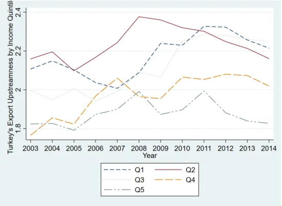
7. Turkey’s Export Upstreamness by Income Quntiles . . . 34

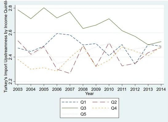
8. Turkey’s Import Upstreamness by Income Quintiles . . . 35

9. The World Log Trade Volume . . . 42

10. Evolution of Turkish Export Upstreamness . . . 43

11. Evolution of Turkish Import Upstreamness . . . 43

12. Standard Deviation of Turkey’s Export Upstreamness for each In-come Quintile . . . 46

13. Standard Deviation of Turkey’s Export Upstreamness for each In-come Quintile . . . 46

14. The Correlation between export-import upstreamness and Real GDP per capita varying across different years . . . 47

15. The Correlation between export-import upstreamness and Rule of Law varying across different years . . . 47

16. The Correlation between export-import upstreamness and Private Credit / GDP varying across different years . . . 48

17. The Correlation between export-import upstreamness and Capital per worker varying across different years . . . 48

(13)

18. The Correlation between export-import upstreamness and TFP

vary-ing across different years . . . 49 19. The Correlation between export-import upstreamness and Years of

(14)

CHAPTER 1 INTRODUCTION

The rising trend in international trade has been the fragmentation of production over the last two decades. The production process now requires sourcing of inputs and components from multiple suppliers. The fact that these multiple suppliers are lo-cated in different countries allows different stages of production to be conducted in different countries. Such a phenomena is called Global Value Chains (GVC) in the literature of international trade. Countries in need of the intermediate goods to com-plete a series of production stages demand inputs in factor markets. This demand driven outbreak has enhanced worldwide trade volume of intermediate goods and raised new policy questions about the position that countries take along the global value chains: Do countries engage in relatively more upstream or downstream trade activities when different manufacturing stages take place in different countries? Can we find a formal way to determine the bilateral trade pattern between any pair of countries? What are the implications of this disintegration of production in terms of country specific factors and variables?

These kinds of questions are particularly important in terms of the strategic trade in-teractions between countries in international markets. Countries try to bring more value added to the products that they import from the world markets, undertaking a great deal of processing in industrial plants to convert them into a high-valued final goods. Therefore, countries which import relatively upstream products, implement

(15)

a sequence of stages on the imported products and finally supply the goods target-ing the final customers in international markets are positioned in the upper portion whereas those who supply raw materials and cannot conduct a large span of produc-tion stages within their domestic borders are posiproduc-tioned in the lower porproduc-tion of global value chains. Hence, terms of trade between countries is largely influenced by the actions of the countries located at relatively upper portions.

The main motivation of this paper is to detect the position of countries in global value chains using the notion of upstreamness. Developed as a metric to measure the distance of a product to its final use, the idea of upstreamness has recently occu-pied the international trade literature and helped researchers determine the position of countries in GVCs. Based on the input-output tables to account for the input us-age in each industry, the measure of upstreamness is used to estimate the number of stages required for a certain industry until it meets the final demand. Therefore, it implicitly explains the characteristics of industries or outputs procured in those in-dustries in terms of their usage as intermediary or final good. The more upstream a product is, the more industries it visits until meeting the final demand. Similarly, the less upstream a product is, the fewer stages are conducted until its usage as a final good.

The upstreamness literature can be traced back to the very first concepts of forward and backward linkages. Blair and Miller (2009) define the forward and backward linkages in terms of the backward or forward production opportunities resulting from an expansion of output in a given sector. An expansion of output in an industry leads that sector to demand more inputs in factor markets. That means it requires a higher level of output produced in the precedent sectors. This is called backward linkages. On the other hand, in case of an expansion, the more output of this sector becomes available for the industries in subsequent stages. Thus, later stages can enjoy an in-crease in the availability of the factor that they use to complete the production of their own products. Working in the opposite direction to the previous terminology,

(16)

it is called forward linkages. The more upstream an industry is, the more it could be said to cause forward linkages. Likewise, if an industry shows a downstream pattern, a positive output shift in that industry induces a demand increase in the already few number of goods it uses as an input. In his search for an optimal policy a country should adopt to develop, Hirschman (1958) argues that countries should invest in the sectors which have the largest amount of forward and backward linkages, supporting a renowned theory of “Unbalanced Growth”. Instead of subsidizing all industries in the economy in a balanced way, he contends that industries generating maximum linkages ought to be developed first. In this respect, those who create the highest number of linkages work as a “self-propelling” mechanism, elevating the production in other sectors and bringing about the maximum benefit to the overall economy.

One of the first efforts to properly compute the upstreamness using Input Output Ta-bles is done by Antrás et al. (2012). They construct the upstreamness measure for 426 industries in United States using 2002 Input-Output (I-O) Tables. They list the most upstream and downstream industries in US in terms of their 6-digit I-O codes. Beside that, using OECD STAN database they compute the industry level ness for a sample of countries and provide the rank correlations of industry upstream-ness between any pair of countries, asserting that upstreamupstream-ness measure is a stable attribute of industries across different countries. Moreover, they apply this concept to trade, calculating the weighted export upstreamness measure for 181 countries be-tween 1996-2005 and try to estimate how the export upstreamness is affected from various country specific factors. One important evidence they come up with is that the presence of good institutions and prevailing rule of law lead countries to export in more downstream industries, meaning that the products they export are considered as final goods within the whole production process.

Moving to another paper focusing on the position of China in GVCs using a firm-level analysis, Chor et al. (2017) deal with the position of Chinese firms in the global value chains, using firms level customs and balance sheet data. They use the notion

(17)

of upstreamness and compute the upstreamness measure for 135 IO sectors from Chinese Input-Output Tables, similar to reasoning of previous paper for the sectors in US. However; they calculate the weighted export and import upstreamness measure using the volume of exports and imports of firms in each specific industry category. More importantly, they introduce a concept of the span of production stages, for-mally UM−UX_{, to capture the span of production stages conducted by Chinese firms} within China. In contrast to the estimation approach used by Antrás et al. (2012), they use firm specific factors in their estimation to account for how the export-import upstreamness and the span of production stages depend on firm specific character-istics. They argue that firm experience, productivity and size are positively corre-lated with the downstream characteristics of firms’ exports. For the other direction, looking for any impact of the enlargement of the span of production stages on firm specific characteristics, they find that firms adopting more production stages in do-mestic economy, i.e. bringing more value added to the imported goods, are exposed to higher level of fixed production costs. In a macro sense, their empirical findings show that Chinese import upstreamness steadily increases between 1992 and 2011 though export upstreamness follows a moderate pattern, which implies that there is a rapid expansion in production stages conducted in China.

Antrás and Chor (2017) take a formal step to combine the empirical exercises on the GVCs with the theoretical models of input flows across countries. They first intro-duce four different measures to elaborate on the methodologies of upstreamness and downstreamness and then provide an empirical investigation on the position of countries between 1995-2011 using 2013 edition of World Input Output Database (WIOD). For 41 countries and 35 industries provided in WIOD for whole period, they present how the GVC positioning of countries changes over time. In their em-pirical assessments, they find that countries whose export composition mainly tar-gets the final consumers, i.e. having a low level of export upstreamness, are indeed those who can contribute much value added to the products that they process in their

(18)

domestic industries, ie., having a higher level of import upstreamness. Finally, they conduct a series of counterfactual analyses to look for how the correlation between export and import upstreamness changes within the context of alternative scenarios such as trade cost reduction and increasing share of spending on service sectors.

This thesis contributes to the literature in two ways. Our first aim is to test the hy-potheses outlined in Antrás et al. (2012) using a more aggregate and recent UN Com-modity Trade data set covering the period from 2003 to 2014. We examine whether the country specific factors can have an impact on the export and import upstream-ness measures using country level and panel regressions. Thus, this paper is in a sense a modification of the results of previous works with an updated data set. Sec-ond, more importantly, we deviate from the existing literature via a bilateral analy-sis to explain how at a point in time the bilateral upstreamness between any pair of countries is affected from the country specific factors, controlling for the source and destination year fixed effects. Based on the empirical findings that the export and import upstreamness of a certain country can vary across its different trade partners over time, we compute the bilateral upstreamness values between any pair of coun-tries and show how these values are affected from country specific factors. Moreover, we add gravity variables provided in Head et al. (2010) to the estimation equations to account for the impact of geographical variables on the production line position of a country against its trade partners. To best of our knowledge, this will be the first attempt to introduce the gravity variables to upstreamness literature. Using such a bilateral framework, we will be able to compare the production line position of any pair of countries and answer how the bilateral upstreamness value of a certain coun-try alters with respect to its trade partners.

The rest of the paper is organized as follows: In the next section, we explain the concept of upstreamness and the reasons why the usptreamness values we calcu-late across countries are reliable predictors to measure the production line positions. Moreover, we describe the data sets used to obtain the weighted export and import

(19)

upstreamness values and explain the procedure of combining data sets subject to our analysis. Third section discusses the empirical findings and how country spe-cific factors are correlated with export and import upstreamness measures using ba-sic correlation plots of average upstreamness values for each country. Moving to a more formal assessment, two different estimation approaches are employed to an-swer whether these country specific factors are effective in changing the position of countries in global value chains (GVCs) and how bilateral upstreamness between any pair of countries respond to these country level characteristics. A separate subsec-tion is also included to point out where Turkey is located in GVCs and moves over time compared to a subset of developed countries (OECD and EU15) and developing countries (BRICS and NewEU). We also conduct a similar analysis by categoriz-ing the trade partners of Turkey across five different income groups. The last section concludes.

(20)

CHAPTER 2 METHODOLOGY AND DATA DESCRIPTION

2.1 Upstreamness Measure

Following Fally (2011) and Antrás et al. (2012), we begin by considering N industry closed economy and extend this to an open economy framework. For each industry i∈ 1, 2, ..., N the value of gross output (Yi) equals the sum of its final use as a final good (Fi) and its use as an intermediate input to other industries (Zi)

Y_i= Fi+ Zi= Fi+ N

∑

j=1

d_{i j}Y_j (2.1)

where di j is the dollar amount amount of sector i’s output needed to produce one dol-lar’s worth of industry j’s output. Iterating this identity, we can write it as

Y_i= Fi+ N

∑

j=1 d_{i j}F_j+ N

∑

j=1 N

∑

k=1 d_ikd_{k j}F_j+ N

∑

j=1 N

∑

k=1 N

∑

l=1 d_ild_lkd_{k j}F_j+ .... (2.2)

Building on this identity, Antrás and Chor (2013) suggest computing the (weighted) average position of an industry’s output in the value chain, by multiplying each term in (2) by their distance from final use plus one and dividing by Yi:

U_i= 1 ·Fi Y_i + 2 · ∑N_j=1di jFj Y_i + 3 · ∑N_j=1∑N_k=1dikdk jFj Y_i + 4 · ∑N_j=1∑N_k=1∑_l=1N dildlkdk jFj Y_i + ... (2.3)

(21)

To implement the open economy adjustment, Antrás et al. (2012) propose the follow-ing expression (see the paper for further discussion), replacfollow-ing di j with:

ˆ d_{i j} = di j

Y_i Yi− Xi+ Mi

(2.4)

where Xiand Miare exports and imports of sector i, respectively.

If Uiis higher, then the industry is further upstream in terms of its contribution to production chains. For instance, petrochemical product (325110)1can be refined in petroleum industry and served to the consumers (2 stages to final use) or it can be used in the Plastic industry (325211) and then used as an input to Alumina refining (33131A) and then finally sold to Automobile industry (336111) to be consumed as a final good (4 stages to final use). On the other hand, Breakfast Cereal (311230) can be directly served to the customers (one stage to final use).

2.2 Data

The main data set we use to classify the position of countries along the GVC is United Nation’s Commodity Trade Data, which provides the export and import value of HS4-code products available for each country from 2003 to 2014. Furthermore, we use the industry-level upstreamness measures computed from 2002 US I-O Tables, which is provided in 6-digit I-O codes for 426 industries. As Antrás et al. (2012) put forward, this upstreamness measure is not considered as only a US specific measure. They compute a spearman rank correlation test for industry level upstreamness of US with countries in European Union and OECD. They find that the rank correlation is always large and positive in all country pairs, verifying the consistency of industry upstreamness across countries. In aggregate terms, this finding makes sense when we consider the share of US in world trade volume as it exports and imports a large

(22)

set of products, providing a better coverage of industries. US is also assumed to be governing frontier technologies, which makes US based measures more standardized compared to the measures constructed based on other countries’ data.2 In terms of the estimation approach, harnessing US based uspreamness measure alleviates any sort of endogeneity concern in the econometric analysis of section 3.4. Therefore, these findings allow us to readily use US industry upstreamness measure to reach a more generalized result for the export and import upstreamness of any country in the world. Formally, we compute the import and export upstreamness measure for each country c in year t ∈ 2003, ..., 2014 in the following manner:

U_ctM= N

∑

i=1 M_cit MctUi, U X ct = N

∑

i=1 X_cit X ctUi (2.5) and U_ctM−U_ctX = N

∑

i=1   M_cit Mct− X_cit X ct  U_i (2.6)

where N is the number of available HS4 products provided in UN Comtrade Data. M_cit (Xcit) denote the import (export) value for product i in year t from destination (for source) country c. Mct = ∑Ni=1Mcit and Xct = ∑Ni=1Xcit are total value of im-ports and exim-ports for that product i in question. The lower value of export upstream-ness shows that the export composition of countries tend to include more down-stream products, ready to be directly served to final consumers. On the other hand, the greater value of that is associated with more upstream exports to the world mar-kets. By expression (2.5), import upstreamness is defined as the weighted average of the upstreamness of imported products, describing whether the import volume com-prises relatively intermediate or final goods. The higher value of import upstream-ness shows that countries purchase more upstream products which require a series of

2_{It is not uncommon to construct standard industry-level measures using U.S. data. For instance,}

Rajan and Zingales (1998) construct an industry-level index of external finance dependence using balance sheet data on U.S. firms.

(23)

production stages to be converted to final use. Therefore, countries having a higher import upstreamness can seize the opportunity to bring more value added on their imported products. As the import upstreamness measure is an analytical tool to char-acterize the distance of imported goods from their final usage, the number of stages operated domestically does not necessarily correlate with the amount of value added created on different types of imported materials. Not all raw material importers could have the essential technology or factors of production to implement value added on the purchased materials from the foreign markets. To rely on a better ground, using the definition in Chor et al. (2017), we suppose that the expression (2.6) captures the span of production stages operated within the domestic borders, showing the depth of the production process for any type of commodity3. Hence, a country having a pos-itive UM− UX is said to process its imported products at a sufficiently great number of industries within its domestic plants before supplying to the world markets. Thus, that country will have a better chance to create more value added on those imported materials at quite a few number of industries, which will subsequently increase the amount of value added in domestic economy.

Note that Uiis the industry level upstreamness for each i from 426 different indus-tries. It might be the case that the data for HS4 products does not exactly match with the upstreamness data, which is made up of upstreamness value for 426 industries and their corresponding I-O code. Thus, to merge the upstreamness data with UN Comtrade data we use a concordance table provided in data replication files of Antrás et al. (2012).4 Then, we obtain a new data set consisting of HS6 product codes and their respective upstreamness values. In order to use this new data set together with UN Comtrade data, we reduce HS6 to HS4 and merge UN Comtrade data with this

3_{Henceforth, we assume that the difference between import and export upstreamness measures is}

used as a proxy for value added produced domestically.

4_{This concordance table gives us a mapping between HS6 type product categories and IO codes.}

When we merge the upstreamness data with concordance table, there are 122 IO codes in master data which do not match with the using data and there are 6 HS6 codes in the using data which do not match with master data. Thus, we take the remaining number of industries which are exactly matched.

(24)

new data set.5 Finally, we obtain a generic data set which shows the upstreamness value of exported and imported products recorded in HS4 category for each country in year t. From this data set, we can readily compute the export and import upstream-ness using (5). Hence, using these usptreamupstream-ness measures, we can compare the po-sition of countries along GVC. For instance, between 2003 and 2014 average export upstreamness of Saudi Arabia is 3.28 whereas Japan has an average export upstream-ness of 2.03. We can interpret these numbers as the number of stages required for the exported products to be converted to final usage. Thus, we can verify that while Japanese exports are processed at most two industries in the importer countries, the products purchased from Saudi Arabia visit at least three sectors until they meet the final demand. This result points out that Japanese exports show a more downstream pattern in world markets. Furthermore, the import upstreamness of Saudi Arabia is 1.98, which is relatively below the value of Japanese import upstreamness, 2.48. Based on these numbers, we can assert that Japan has a positive span of production stages, meaning that it has a better capability to induce value added on the imported products compared to what Saudi Arabia can do, which places Japan at a higher posi-tion along the global value chains.

In order to account for the variations in export and import upstreamness of each country, we use the following country characteristics. To look for how the educa-tion attainment affects the export and import upstreamness, we use Barro and Lee (2013)’s education attainment data, which is available from 1950 to 2010 in 5-year intervals. Since our main data set covers the period from 2003 to 2014, we fill this period paying attention to the proximity of the years available. For instance, we use the estimate years of schooling in 2005 for the interval [2003,2007] and the estimate years of schooling in 2010 for the interval [2008,2014]. To understand how the ratio

5_{HS6 is a broader product-level classification than HS4. Thus, when reducing HS6 to HS4, there}

might be more than one upstreamness value corresponding to each HS4 code. To circumvent this multiplicity problem, we take the average of upstreamness measure and obtain a new data set in which each HS4 product code has a unique upstreamness value.

(25)

of private credit to GDP as an instrument for financial development has an impact on the span of production stages, we use World Global Financial Database from Bartels-man et al. (2013). This is also available between 2003 and 2014. Additionally, we in-clude real GDP per capita from World Development Indicators (WorldBank, 2019) in our analysis to understand how the trade upstreamness evolves over time in response to the changes in per capita real GDP. Using the same data set, we also incorporate total factor productivity to observe how the productivity gains could have an impact on country level upstreamness. Antrás et al. (2012) augment the physical capital per worker, which is constructed using perpetual inventory method, from Penn World Ta-bles (Feenstra et al., 2015), into their estimation approach to measure the response of export upstreamness to the changes in factor endowments. We also use the same variable from PWT. As the production stages are largely affected from the quality of the contracts and institutions, we use the estimate of rule of law in the specified time period using World Governance Indicators from Kaufmann et al. (2017).

(26)

CHAPTER 3 EMPIRICAL RESULTS

3.1 An Overview on Initial Findings

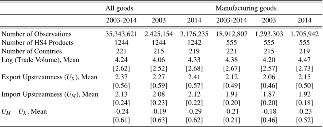
Table 1: Summary Statistics

All goods Manufacturing goods

2003-2014 2003 2014 2003-2014 2003 2014 Number of Observations 35,343,621 2,425,154 3,176,235 18,912,807 1,293,303 1,705,942

Number of HS4 Products 1244 1244 1242 555 555 555

Number of Countries 221 215 219 221 215 219

Log (Trade Volume), Mean 4.24 4.06 4.33 4.38 4.20 4.47

[2.62] [2.52] [2.68] [2.67] [2.57] [2.73] Export Upstreamness (UX), Mean 2.37 2.27 2.41 2.12 2.06 2.15

[0.56] [0.59] [0.57] [0.49] [0.46] [0.50] Import Upstreamness (UM), Mean 2.13 2.08 2.12 1.91 1.87 1.92

[0.24] [0.23] [0.22] [0.20] [0.20] [0.18]

UM−UX, Mean -0.24 -0.19 -0.29 -0.21 -0.18 -0.23

[0.61] [0.63] [0.62] [0.21] [0.46] [0.52]

Notes: Summary Statistics are reported for all goods and manufacturing goods available in UN Comtrade Database. The values in square brackets denote standard deviations. The values for manufacturing goods are generated using NBER-CES Manufacturing Industry Database from Becker et al. (2016). It comprises a list of 473 NAICS industries similar to 6-digit IO codes. Using a concordance mapping provided in BEA website, we create another concordance ta-ble between HS6 and availata-ble NAICS codes. Merging this regenerated concordance tata-ble with upstreamness measures, the upstreamness values of manufacturing goods are expressed in terms of HS6 codes. Finally, after reducing HS6 to HS4 and applying a similar reasoning mentioned in footnote 3, upstreamness measures for HS4 manufacturing products (555 in total) are obtained. The mean of log (trade volume) is calculated only within the sample of manufacturing goods.

Table 1 presents the summary statistics on the UN Comrade data set and upstream-ness measures we compute using the procedure in the data section with respect to the entire period (2003-2014), initial year (2003) and terminal year (2014). The average log world trade volume has drastically increased during this 12-year period and its dispersion around the mean level has also experienced a significant rise. The first im-plication for the overall position of countries in GVC comes from the fourth to six rows in Table 1. On average export pattern is relatively more upstream than import

(27)

pattern for the entire time period. That is, countries mostly sell products, which are also processed by others to enhance the amount of value added. However, the coun-tries are more scattered around the mean level of export upstreamness than they are around that of import upstreamness. This could happen if there is a significant differ-ence between export upstreamness of countries. While a group of countries produces goods which are directly put into final use, others might export products necessarily used in intermediate stages of the production process. This discrepancy can account for the pattern of trade between a raw material supplier who cannot add much value added to its exports and an importer who contributes to the imported products and converts them to final usage after a certain number of stages. For the case of import upstreamness, the position of countries in production line is more moderate.

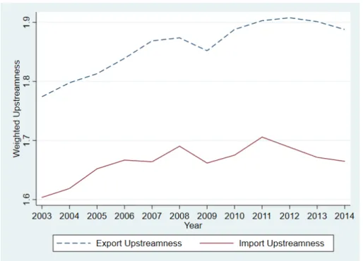
Figure 1: The Movement in World’s Production Line Position

To understand how on average the production line position of the countries changes over time, Figure 1 presents the world export and import upstreamness weighted by the countries’ income level for all goods provided in UN Comtrade. Thus, the export and import upstreamness of high income level countries have a larger impact in de-termining the shape of the graphs in Figure 1. Similar to what we observe in Table 1, exports are on average more upstream than imports. However; they almost move

(28)

parallel to each other during the specified time period. Both of the lines show an in-creasing trend up to 2008. However; with the advent of the global financial crisis, we could see a fall both in both of the upstreamness measures, implying that the ex-ported products show a tendency to be supplied more downstream and the share of intermediate goods in the trade volume of countries declines as well. Because the production level contracts all over the world, this reflects the decrease in the volume of trade for input materials. Though import upstreamness recovers after the crisis period, it steadily falls in the period starting with 2011. Exports, on the other hand, become more upstream after the crisis period, but start targeting final customers es-pecially towards the end of our time period.

Table 2: Upstreamness of Manufacturing Exports by Country Income Quartiles

Income quartile Mean S.D. Min Max

Bottom 2.11 0.58 1.12 4.15

2nd 2.22 0.47 1.07 4.16

3rd 2.17 0.48 1.09 3.71

Top 2.08 0.41 1.04 3.06

Table 3: Upstreamness of Manufacturing Imports by Country Income Quartiles

Bottom 1.90 0.20 1.14 2.92

2nd 1.96 0.18 1.22 2.44

3rd 1.93 0.18 1.38 2.47

Top 1.88 0.20 1.19 2.65

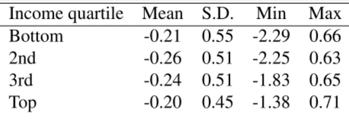
Table 4: Span of Production Stages (UM−UX) of Manufacturing Goods by Country Income

Quartiles

Bottom -0.21 0.55 -2.29 0.66

2nd -0.26 0.51 -2.25 0.63

3rd -0.24 0.51 -1.83 0.65

Top -0.20 0.45 -1.38 0.71

Following the empirical strategy of Antrás et al. (2012), we consider the summary statistics of export and import upstreamness by country income groups, as described

(29)

in Table 2 and 3. Additionally, we extend this analysis including the summary statis-tic of the difference between import and export upstreamness to drive some impli-cations on the number of production stages operated domestically (Table 4). Coun-tries are grouped into income quartiles based on the average log PPP-adjusted Real GDP per capita over 2003-2014, from World Bank World Development Indicators. The average upstreamness of all these three measures togerther with their respective standard deviations and min-max values within each income quartile are reported in Table 2, 3 and 4, respectively.1

Here the interesting point is that poorer countries appear to be exporting in more up-stream industries compared to richer ones. Therefore, richer countries tend to export products aimed to be directly served in final markets. Another interesting result of Table 2 is that the standard deviation of export upstreamness in each income group decreases as it moves from bottom to top. Countries in the bottom quartile thus vary in terms of the average position they occupy in global production lines. To illustrate, Haiti and Zambia are both included in bottom income group. However; based on the export composition of goods they supply to world markets in 2014, we can see that their respective export upstreamness demonstrates a large difference (1.14 vs 3.98). This difference can be attributed to the types of products which occupy a larger share in the export content of both countries. While coffee, as a perishable food served to the final customers after few number of stages, constitutes a great portion of the ex-ports of Haiti, Zambia is a major exporter of unrefined copper, which is processed by a greater number of industries until meeting the final demand. When we consider upstreamness of manufacturing imports by each income quartile, we cannot observe such a pattern. If we have a look at Table 4, we also see a slight increase in mean

1_{When we download the PPP-adjusted GDP per capita from World Bank’s Data Bank and merge}

it with the upstreamness data, there are 385 observations in the upstreamness data that cannot be matched with the GDP per capita data set. Similarly, 644 observations from the second data set are missing in the fist one. Thus, we move on our analysis using the remaining number of 2216 obser-vations, which comprise 189 countries between 2003-2014. Distributing the export and import up-streamness into 4 income group in ascending order yields almost 47-48 countries for each quartile.

(30)

level of UM− UX, arguing that richer countries might have a potential to process the upstream import materials until targeting the foreign markets. The finding that top group has the maximum possible value of this difference is also in line with the observation that considerable portion of the procurement process of manufacturing goods occurs in the rich countries.

3.2 Correlation with Country Characteristics

This subsection mainly depicts how the average export and import upstreamness are correlated with the average country characteristics between 2003-2014. 2 Figure 23 indicates how average export and import upstreamness are correlated with the esti-mates of rule of law. Countries who have a higher quality of governance index tend to export in more downstream industries, consistent with the findings in Antrás et al. (2012). On the other hand, there is not a certain pattern for average import upstream-ness.

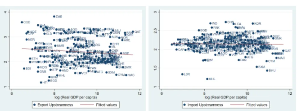
Another important feature in characterizing the position of countries in production line is to look at how upstreamness measures respond to changes in real GDP per capita. Figure 3 gives us a blurring picture between the average upstreamness and log of Real GDP per capita, PPP adjusted. Though we can observe a slightly downward sloping line for export upstreamness, such a trend disappears for import upstream-ness. Thus, consistent with what we find in Table 2, rich countries have a propensity to export more downstream products. Furthermore, the years spent in school on av-erage have a positive impact on the downstreamness of the exported products (Figure

2_{We take the average of export and import upstreamness between 2003-2014. The same procedure}

is also applicable for the estimates of rule of law and log of Real GDP per capita. Here the fact that Barro-Lee’s education attainment data is available for 5-year intervals drives us to calculate average years of schooling between 2003 and 2014 using the values in 2005 and 2010, using the procedure described above.

(31)

4), implying that investment in education might play a role in changing the position of a country’s production line position. The observation that export upstreamness is more responsive to the country level characteristics than import upstreamness might suggest that country characteristics mostly affect the span of production stages from production channel rather than demand channel.

Figure 2: Export-Import Upstreamness and Rule of Law

Figure 3: Export-Import Upstreamness and Real GDP per capita

Figure 4: Export-Import Upstreamness and Years of Schooling

3.3 Econometric Analysis

The subsection 3.2 was a rough treatment of the effect of country characteristics on average upstreamness values using a cross country examination. This section

(32)

em-braces a more formal approach in analyzing the upstreamness measures and other country characteristics. Our estimation consists of two approaches:

3.3.1 Estimation with Country Level Factors

The first approach comprises two main specifications, in the first of which we aim to do a cross country regression following estimation procedure of Antrás et al. (2012), taking the average of all variables over whole period, to examine how the export and import upstreamness are related to the country characteristics and in second of which we intend to do a fixed-effect panel OLS estimation. Formally,

Y_c= α + β Zc+ εc (3.1)

where Yc is one of the average country upstreamness variables in n

U_cM,U_cX,U_cM− U_cXo. Zcis a combination of variables, including the average of log of Real GDP per capita, private credits/GDP, years of schooling, log of physical capital per worker and the estimate of rule of law during the specified time period.4 εcis the error compo-nent for any country c. For the second specification, we consider the following panel regression for all t ∈ 2003, ...2014:

Y_ct = α + δc+ γt+ ΓZct+ εct (3.2)

where the dependent variables are the upstreamness measures (U_ctM,U_ctX and U_ctM− U_ctX) for each country c at time t. δcand γt are country and year specific fixed effects. Zis the same generic vector depending on time, additionally including total factor productivity from PWT. The last term is the usual cluster error by country and year.

4_{Here notice that the variable for years of schooling is again calculated as the average of the filled}

(33)

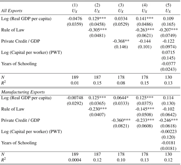
Table 5: Export Upstreamness and Country Characteristics

(1) (2) (3) (4) (5) All Exports UX UX UX UX UX

Log (Real GDP per capita) -0.0476 0.129*** 0.0334 0.141*** 0.109 (0.0359) (0.0458) (0.0529) (0.0486) (0.165) Rule of Law -0.305*** -0.263*** -0.207***

(0.0481) (0.0621) (0.0749) Private Credit / GDP -0.368** -0.144 -0.122

(0.146) (0.101) (0.0974) Log (Capital per worker) (PWT) 0.0715

(0.145) Years of Schooling -0.0377 (0.0243) N 189 187 178 178 130 R2 0.01 0.15 0.08 0.15 0.13 Manufacturing Exports

Log (Real GDP per capita) -0.00748 0.125*** 0.0644* 0.125*** 0.114 (0.0292) (0.0365) (0.0333) (0.0375) (0.130) Rule of Law -0.230*** -0.145*** -0.102

(0.0407) (0.0508) (0.0642) Private Credit / GDP -0.360*** -0.233*** -0.246***

(0.0821) (0.0608) (0.0618) Log (Capital per worker) (PWT) -0.00223 (0.120) Years of Schooling -0.0181 (0.0181) N 189 187 178 178 130 R2 0.0004 0.12 0.10 0.13 0.12

Notes: ***,**, and * denote significance at the 1%, 5% and 10% levels respectively. The values in parentheses are robust standard errors.

(34)

Table 5 tests the same hypotheses put forward in Antrás et al. (2012) to understand in which direction the country level characteristics can have an impact on the export upstreamness for all and manufacturing goods. Considering the second column, we can verify that as the strength of contracting institutions rises, the countries export relatively more downstream though per capita GDP works in the opposite direction. As countries move to the higher stages of income, their exports become relatively more upstream. The usage of private credits over GDP, as a proxy for financial devel-opment has a negative and significant effect only in the third column when we do the estimation for all goods. However; when we pay a close attention to the estimation done only using manufacturing goods, we can observe that it becomes significant and theoretically consistent in all models, suggesting that export upstreamness for man-ufacturing goods is more sensitive to the financial development level than it is for all goods, the rest of which consists of mostly agricultural and service products. One possible explanation is that as the producers increase the amount of credit they bor-row, they might be willing to invest loans in the manufacturing sectors, which have relatively more favorable terms of trade than the sectors of agriculture or service. This upward investment shift can create an incentive for the manufacturers to operate the upper stages of production in domestic plants before supplying to foreign markets during the intermediate stages. In contrast, they might have less incentive to export agricultural goods after conducting the final stages in their home countries or since the output of the service sector is mainly served to domestic markets, they might not be willing to supply service goods to foreign markets. Thus, the pure effect of man-ufacturing goods can be more precise in reducing the export upstreamness. The es-timate of rule of law has a significant and negative effect on export upstreamness of manufacturing goods though the statistical significance of its coefficient consider-ably falls in the last model. Model 5 also allows us to make some inference on how investing in human capital can play a role in a country’s production line position. Though we cannot observe a statistically significant impact, as the years of schooling

(35)

increases, the export activities on average seem to be targeting final demand. How-ever; the significance level is not sufficient to reach this conclusion. The results in Table 5 are consistent with what Antrás et al. (2012) find testing the same specifica-tions. Though the explanatory power of the coefficients of private credits over GDP is slightly lower compared to their results, the coefficient of rule of law is more sig-nificant in each of the models tested above.

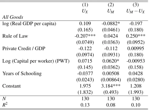
Table 6: Upstreamness and Country Characteristics

(1) (2) (3)

U_X U_M U_M−UX

All Goods

log (Real GDP per capita) 0.109 -0.0882* -0.197 (0.165) (0.0461) (0.180)

Rule of Law -0.207*** 0.0424 0.250***

(0.0749) (0.0363) (0.0952)

Private Credit / GDP -0.122 -0.112 0.00995

(0.0974) (0.0931) (0.180) Log (Capital per worker) (PWT) 0.0715 0.0620* -0.00953

(0.145) (0.0362) (0.158) Years of Schooling -0.0377 0.00508 0.0428 (0.0243) (0.00864) (0.0280) Constant 1.975 3.184*** 1.208 (1.832) (0.493) (1.993) N 130 130 130 R2 0.13 0.08 0.10

Notes: ***,**, and * denote significance at the 1%, 5% and 10% levels respectively. The values in parentheses are robust standard errors.

Table 6 introduces the import upstreamness and the span of production stages, UM− U_X, in addition to the last specification of Table 4. The only variables that could have an impact on import upstreamness are GDP per capita and capital per worker though their explanatory powers are less precise. The increase in capital per worker is asso-ciated with an rise in import upstreamness but model (3) does not support our pre-vious claim that high income countries tend to contribute more value added to the imported products. Still, it yields an important implication for the production stages conducted within domestic industries. The better institutions allow countries to pro-cess the intermediate stages within their own boundaries, which might trigger an

(36)

in-crease in the value of production.

Table 7 reveals the estimation results for specification (8), tested with country and year specific effects. It also includes total factor productivity from PWT. The impact of GDP per capita on upstreamness measures is still in line with the results of Table 6 and does not match with our prior claim. The coefficient of rule of law in the model for export upstreamness is theoretically meaningful, but insignificant. We also do not see the effect of total factor productivity in explaining the variations in produc-tion line posiproduc-tion. The models other than (3) and (4) produce significant estimates for years of schooling but they are inconsistent with theoretical predictions. The mod-els of import upstreamness (3-4) fail to truly capture the impact of rule of law on import upstreamness but still they make sense considering the finding that higher capital intensity per worker could lead a certain country to import relatively interme-diate goods from the world markets (Model 3-4). Yet, the second model of Table 6 together with third and fourth models of Table 7 should be interpreted cautiously as “the relevance of these country variables in explaining trade patterns is thus specific to the supply side, and does not appear to be driven by differences in the composi-tion of demand” (Antrás et al., 2012:16 in longer version). Therefore, country-level characteristics are more meaningful and prevailing in production channel instead of demand channel.

3.3.2 The Impact of Country Level Characteristics on Bilateral Upstreamness

Theoretically inconsistent and imprecise estimates of Table 5 and 6 do not bring con-vincing results in analyzing the direction of correlation from country level variables to upstreamness measures. Thus, rather than looking at the overall variation in up-streamness measures in response to country characteristics, we propose that a coun-try’s export and import upstreamness measure could be varying across its different trade partners. For instance, Turkey could concentrate on the exports of final goods

(37)

T able 7: P anel Regr essions (1) (2) (3) (4) (5) (6) UX UX UM UM UM − UX UM − UX Log (Real GDP per capita) 0.131* 0.182*** -0.169** -0.0681 -0.299*** -0.250*** (0.0705) (0.0639) (0.0658) (0.0582) (0.0882) (0.0805) Rule of La w -0.0135 -0.0248 -0.0496** -0.0781*** -0.0361 -0.0533 (0.0424) (0.0396) (0.0213) (0.0210) (0.0477) (0.0447) Pri v ate Credit / GDP 0.000493 0.00442 -0.00931 0.0136 -0.00981 0.00918 (0.0327) (0.0314) (0.0424) (0.0388) (0.0400) (0.0367) Log (Capital per w ork er) 0.160** 0.138** 0.258*** 0.221*** 0.0986 0.0826 (0.0743) (0.0650) (0.0424) (0.0414) (0.0840) (0.0728) TFP at constant national prices (2011=1) 0.0588 0.0558 -0.0877 -0.0914 -0.146 -0.147 (0.100) (0.0998) (0.0833) (0.0834) (0.114) (0.115) Y ears of Schooling 0.0666*** 0.0610*** 0.0113 0.0142 -0.0553*** -0.0468*** (0.0162) (0.0133) (0.00945) (0.00924) (0.0180) (0.0143) Country Fix ed Ef fects? Y es Y es Y es Y es Y es Y es Y ear Fix ed Ef fects? Y es No Y es No Y es No N 1240 1240 1240 1240 1240 1240 R 2 0.93 0.93 0.85 0.85 0.93 0.93 Notes: ***,**, and * denote significance at the 1%, 5% and 10% le v els respecti v ely . The v alues in parentheses sho w rob ust stan-dard errors. Model (1) and (2) tak e export upstreamness, model (3) and (4) tak e import upstreamness and model (5) and (6) tak e UM − UX , span of production stages, as a dependent v ariable.

(38)

to less developed countries while its exports tend to comprise more raw materials when it exports to more developed countries, necessarily increasing its export up-streamness. On the other hand, it could bring more value added to the imported prod-ucts from the poorer countries, but there might not exist much opportunities to pro-cess the goods imported from richer countries. This fact could also be sensitive to the changes in country level factors. The relative production line position of a country might alter with respect to its trade partners in case of a change in not only its own but also its trade partners’ characteristics. This finding leads us to employ a bilateral approach in examining such a direction of causality. In what follows, we define the bilateral upstreamness measurefrom the perspective of exportation. For any source country i and destination country j at time t

U_{i jt} = N

∑

k=1 X_{i jkt} X_{i jt} Uk

where X_{i jkt} is the volume of exports from the source country i to the destination country j for a specific product category k at time t. Xi jt is the total volume of ex-ports. Similar to the formula we use to define the export and import upstreamness, we weight the volume of exports from i to j by the industry upstreamness measure of N-available number of product k. Similarly, we can also define the bilateral up-streamness from the perspective of importation:

Ui jt = N

∑

k=1 M_jikt Mjit U_k

where Mjikt is the volume of imports to the destination country j from the source country i for a specific product category k at time t. Mjit is the total volume of im-ports.

To illustrate our findings, we return to comparison of Japan and Saudi Arabia in global value chains. Previously, we examined the average position of each of these countries taking into account their export and import pattern with the rest of the

(39)

world. Now we consider the bilateral trade pattern between Japan and Saudi Ara-bia at a point in time, particularly in 2014. Import upstreamness of Saudi AraAra-bia to Japan (export upstreamness of Japan to Saudi Arabia) is around 1.73 whereas the im-port upstreamness of Japan to Saudi Arabia (exim-port upstreamness of Saudi Arabia to Japan) is around 3.31. This implies Japan can contribute to the value of the materials it purchases from Saudi Arabia within more than three sectors while Saudi Arabia mostly purchases goods from Japan ready to be sold to final customers and cannot bring much value added to its imports from Japan.

Our approach in this section consists of the regression equations accounting for the bilateral upstreamness at a point in time between a source and a destination country. We aim to test two different bilateral specifications. The main purpose of conduct-ing the first bilateral analysis is to explain how the upstreamness between a source and a destination country changes in response to the variables in source or destina-tion countries, controlling for destinadestina-tion-year and source-year fixed effects. In ad-dition to that, our estimation equations consist of gravity variables5to account for the geographical impact on bilateral production line position between two different countries. Thus, we can explain how GDP per capita, rule of law, the ratio of private credits to GDP, capital stock per worker, total factor productivity and years of school-ing in a certain country could affect the bilateral upstreamness between any trade partners, controlling for the country fixed effects and gravity terms. Formally,

Ui jt = α0+ α1Xit+ α2Zi j+ Γjt+ εi jt (3.3)

5_{CEPII Gravity Database is harnessed to include the gravity variables for estimation procedure}

from Head et al. (2010). The variables of interest are the distance (km) between the source and des-tination country, a dummy variable for common language to explain whether the same language is spoken between the trade partners, a dummy variable for contiguity to show if there is a common bor-der and a dummy variable for the presence of a free trade agreement.

(40)

and

U_{i jt} = β0+ β1Xjt+ β2Zi j+ Γit+ ui jt (3.4)

where the dependent variable is the bilateral upstreamness measure between a source country i and a destination country j at time t. Xit (Xjt) is a vector of country specific factors in source country i (destination country j). Zi j is a vector of gravity variables between a source i and destination j. Γjt and Γit denote the destination and source fixed effects at time t, respectively.

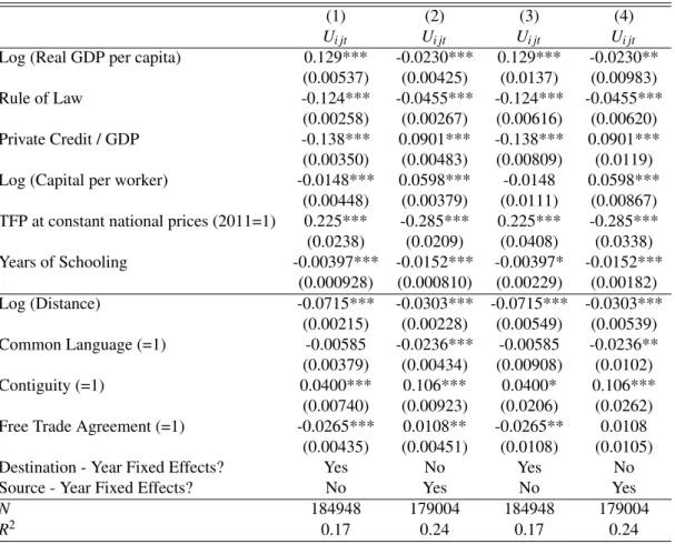
Table 8: The Impact of Source and Destination Specific Variables on Bilateral Upstreamness

(1) (2) (3) (4) Ui jt Ui jt Ui jt Ui jt

Log (Real GDP per capita) 0.129*** -0.0230*** 0.129*** -0.0230** (0.00537) (0.00425) (0.0137) (0.00983) Rule of Law -0.124*** -0.0455*** -0.124*** -0.0455***

(0.00258) (0.00267) (0.00616) (0.00620) Private Credit / GDP -0.138*** 0.0901*** -0.138*** 0.0901***

(0.00350) (0.00483) (0.00809) (0.0119) Log (Capital per worker) -0.0148*** 0.0598*** -0.0148 0.0598***

(0.00448) (0.00379) (0.0111) (0.00867) TFP at constant national prices (2011=1) 0.225*** -0.285*** 0.225*** -0.285*** (0.0238) (0.0209) (0.0408) (0.0338) Years of Schooling -0.00397*** -0.0152*** -0.00397* -0.0152*** (0.000928) (0.000810) (0.00229) (0.00182) Log (Distance) -0.0715*** -0.0303*** -0.0715*** -0.0303*** (0.00215) (0.00228) (0.00549) (0.00539) Common Language (=1) -0.00585 -0.0236*** -0.00585 -0.0236** (0.00379) (0.00434) (0.00908) (0.0102) Contiguity (=1) 0.0400*** 0.106*** 0.0400* 0.106*** (0.00740) (0.00923) (0.0206) (0.0262) Free Trade Agreement (=1) -0.0265*** 0.0108** -0.0265** 0.0108

(0.00435) (0.00451) (0.0108) (0.0105) Destination - Year Fixed Effects? Yes No Yes No Source - Year Fixed Effects? No Yes No Yes N 184948 179004 184948 179004 R2 0.17 0.24 0.17 0.24

Notes: ***,**, and * denote significance at the 1%, 5% and 10% levels respectively. The values in paren-theses show robust standard errors, except in column (3) and (4) where they are clustered by source and destination country instead.

Table 8 displays the estimates of coefficients in both specifications above. Model (1-2) use robust standard errors while (3-4) cluster the standard errors by source-destination country pairs to take into account any inflation in standard errors

(41)

result-ing from the unobservable impact of possible clusterresult-ing of trade partners . Though the significance of the estimates comparably falls in models (3-4), they could still ex-plain the variation in bilateral upstreamness. One of the stark findings from models 1 and 3 is that an increase in per capita real GDP in a source country is associated with an increase in its export upstreamness, i.e., import upstreamness of the desti-nation country given that destidesti-nation specific characteristics are fixed. Thus, as the income level of the exporter country increases, its trade partner tends to import more upstream products. The strength of contracting institutions and financial develop-ment in exporting countries can induce them to specialize in the production of goods directly targeting the final markets in importer countries. If the productivity rises in the source country, import upstreamness of the destination country also increases, meaning that the share of intermediate goods in importer’s trade volume significantly rises. The investment in human capital in exporter country slightly changes its export pattern, making the export composition more downstream. Here the gravity terms are also effective in changing the bilateral position between two trade partners. As the source and destination countries are located further away from each other, this can make the types of products exported by the source country more downstream. This result is consistent with the implications of gravity models on the impact of distance on the value of products exported to foreign markets. Increasing distance can lead the producers in the source country to change the composition of exports towards high value commodities, for which it is more profitable to incur fixed and variable trade costs of servicing the remote markets. Thus, the incentive of exporting high value commodities to remote destinations can increase the number of subsequent stages of production undertaken in domestic plants and induce a more downstream pattern for the types of products subject to exportation. Furthermore, free trade agreements can also allow the exporter countries to supply more downstream goods in the destination markets. If there is a common border between the trading partners, we could observe a rise in the import upstreamness of destination countries relative to exporters.

(42)

The other models in Table 8 (2 and 4) consider the impact of destination specific fac-tors on bilateral upstreamness, taking the characteristics of source country at time t fixed. As the destination country gets richer and the quality of institutions increases, it imports more downstream products from its exporter partner. The share of private credits in GDP significantly improves its ability to import more upstream products. While the intensity of capital per worker in importer country might create an impetus to enlarge the number of production stages conducted within its home plants, the pro-ductivity increase works in the other way around. The increase in years of schooling in the destination country seem to be leading the source country to concentrate on the sale of final goods. The inclusion of gravity terms also yields interesting results for the second specification. The increase in the distance between source and destina-tion country allows the source country to export more downstream products. Unlike the first specification, the coefficient for common language dummy is significant for this model. If the trading partners share the same language, this could allow the ex-porter country to sell final products to the imex-porter. In case of a common border, we can observe a rise in the import upstreamness of the destination country. When we examine the effect of signing a free trade agreement between two trade partners, we see alternating results depending on the fixed effects we use in the estimation. If we fix the destination-year effects, we find a relatively more downstream characteristics for the products of exporter country. However; fixing the source-year effects, free trade agreement might bring about a rise in the import upstreamness of the destina-tion country.

We also test the following specification to combine the bilateral estimation equations above to examine the joint impact of source and destination specific variables on bi-lateral upstreamness in one specification:

U_{i jt}= δ0+ δ1Xit+ δ2Xjt+ δ3Zi j+ Γi+ Γj+ γt+ ei jt (3.5)

(43)

source i and destination j at time t. Zi j is the gravity variables in the first specifi-cation. We also include Γiand Γj to control for the source and destination country fixed effects6. Time fixed effect γt is also added to our specification. ei jt is the usual error term.

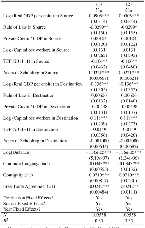
Table 9 displays the estimation results of this specification. Using a similar strategy to the previous bilateral analysis, we also test the model with clustered standard er-rors to account for the impact of any unobserved factors regarding with source desti-nation country pairs. Even if the standard errors are inflated due to the usage of clus-tering, the coefficients do not lose their statistical significance tough there is a mild fall in the explanatory power of TFP for the source country. The increase in income level and years of schooling in source country appear to be leading to more upstream exports while the strength of institutions and productivity gains bring about more downstream exports. By definition of bilateral upstreamness, the same variables affect the import upstreamness of the destination country in the other way around. When we examine the impact of destination characteristics on the bilateral upstream-ness, real income level and capital intensity per worker are the only effective vari-ables. The higher income level of the destination causes it to import less upstream products whereas the higher capital intensity allows it to import more upstream prod-ucts. When we consider the gravity variables, they are totally consistent with the results previous table. The distance between two trade partners, the presence of a common language and a free trade agreement reduce the export upstreamness of the source country. If trade partners are two neighbor countries with a common border, this would help the destination country import relatively more upstream products.

(44)

Table 9: The Joint Impact of Source and Destination Specific Variables on Bilateral Upstreamness

(1) (2)

Ui jt Ui jt Log (Real GDP per capita) in Source 0.0903*** 0.0903***

(0.0314) (0.0344)

Rule of Law in Source -0.0299** -0.0299*

(0.0150) (0.0155) Private Credit / GDP in Source 0.00104 0.00104 (0.0120) (0.0122) Log (Capital per worker) in Source 0.0131 0.0131

(0.0262) (0.0292)

TFP (2011=1) in Source -0.106** -0.106**

(0.0432) (0.0480) Years of Schooling in Source 0.0221*** 0.0221***

(0.00568) (0.00621) Log (Real GDP per capita) in Destination -0.136*** -0.136*** (0.0305) (0.0352)

Rule of Law in Destination 0.00606 0.00606

(0.0132) (0.0140) Private Credit / GDP in Destination -0.00498 -0.00498 (0.0131) (0.0137) Log (Capital per worker) in Destination 0.118*** 0.118***

(0.0239) (0.0273) TFP (2011=1) in Destination -0.0149 -0.0149 (0.0356) (0.0420) Years of Schooling in Destination -0.001000 -0.001000

(0.00644) (0.00682)

Log(Distance) -1.36e-05*** -1.36e-05***

(5.19e-07) (1.24e-06)

Common Language (=1) -0.0343*** -0.0343***

(0.00555) (0.0132)

Contiguity (=1) 0.0710*** 0.0710***

(0.00817) (0.0230) Free Trade Agreement (=1) -0.0242*** -0.0242**

(0.00484) (0.0111)

Destination Fixed Effects? Yes Yes

Source Fixed Effects? Yes Yes

Year Fixed Effects? Yes Yes

N 109558 109558

R2 0.35 0.35

Notes: ***,**, and * denote significance at the 1%, 5% and 10% levels respec-tively. The first model is estimated using robust standard errors whereas in the second model they are clustered by source destination country pairs instead.

(45)

3.4 The Production Line Position of Turkey

3.4.1 The Movement relative to OECD, BRICS and EU members

The computation of bilateral upstreamness between any pair of countries allows us to keep track of how production line position of a certain country or a block of coun-tries changes over time. In this section, we compare the evolution of Turkey’s pro-duction line position with both developed and developing country groups. For de-veloped group, we consider the countries in OECD7and 15 members of European Union8. For developing country groups, we consider BRICS9and new members of European Union10. Taking the average of all countries involved in each group at a point in time, we sketch how Turkish position on average evolves over time against these blocks. This will allow us to portray the changes in relative position of Turkey in global value chains with respect to two different income groups.

Figure 5 illustrates the movement of Turkish export upstreamness compared to both developed and developing groups. On average Turkish exports to the rest of the world are processed by at least two industries and it shows the most drastic change among all the other country groups during the period between 2006 and 2011. Turkish ex-ports, especially after 2006, become more upstream, concentrating on the sale of in-termediate goods in world markets. While this pattern increasingly continues until

7_{Australia, Austria, Belgium, Canada, Chile, Czech Republic, Denmark, Estonia, Finland, France,}

Germany, Greece, Hungary, Iceland, Ireland, Israel, Italy, Japan, Korea, Latvia, Lithuania, Luxem-bourg, Mexico, Netherlands, New Zealand, Norway, Poland, Portugal, Slovak Republic, Slovenia, Spain, Sweden Switzerland, the United Kingdom and the United States. Since Turkey is also a mem-ber of OECD, we exclude that to obtain the average of remaining countries. OECD (2019).

8_{Austria, Belgium, Denmark, Finland, France, Germany, Greece, Ireland, Italy, Luxembourg, the}

Netherlands, Portugal, Spain, Sweden and the United Kingdom. European-Commission (2019)

9_{Brazil, Russia, India, China and South Africa.}

10_{EU countries which became members after 2004 enlargement: Czech Republic, Estonia, Cyprus,}

Latvia, Lithuania, Hungary, Malta, Poland, Slovakia, Slovenia, Romania, Bulgaria and Croatia (Euro-pean Commission, 2019).

(46)

(a) Panel A: Developed Group (b) Panel B: Developing Group

Figure 5: Evolution of Export Upstreamness

2011, Turkish exports start targeting final demand during the last three years in our data set. Turkey together with BRICS is located in the intermediate stages of pro-duction chains compared to the other country blocks on average. As we observe a relatively flat movement of BRICS countries, EU15 and OECD countries have a ten-dency to follow a more downstream pattern in exporting. The fact that EU15 coun-tries follow the most downstream pattern highlights an important implication: export composition of the most developed EU members is mostly final good oriented in in-ternational markets.

(a) Panel A: Developed Group (b) Panel B: Developing Group

Figure 6: Evolution of Import Upstreamness

The picture becomes more interesting when we analyze how Turkish import up-streamness on average moves compared to the same set of countries (Figure 6) and investigate which one of these country groups resembles Turkey in terms of the pro-duction line position. While OECD and EU15 members move parallel to each other, Turkey and BRICS countries follow an exactly opposite pattern. Turkey similar to BRICS average imports mostly upstream products from world markets. Towards

(47)

2014, as both of them experience a fall in export upstreamness, accompanied by a rise in import upstreamness, they could have increased the number of production stages conducted domestically. Thus, when we consider the position of Turkey in GVCs, it is more similar to BRICS countries than EU15 or OECD members. Apart from this, Turkish imports on average are slightly more upstream than those of BRICS. Even though this pattern vanishes during the period between 2011-2012, Turkey earns its previous position back, pursuing a more upstream pattern 2013 onward.

3.4.2 Upstreamness of Turkey by Income Quintiles

Figure 7: Turkey’s Export Upstreamness by Income Quntiles

Using the bilateral upstreamness between Turkey and its trade partners, we can keep track of how Turkey’s export and import upstreamness changes over time across dif-ferent income groups. Here we divide the income level of Turkey’s trade partners into 5 different group, each of which yields one quintile for a given year. While Q1 includes the poorest trade partners of Turkey, Q5 consists of the richest group of countries. Figure 7 captures the evolution of Turkey’s export upstreamness against