The Journal of Applied Business Research – January/February 2015 Volume 31, Number 1
Power Laws In Financial Markets:
Scaling Exponent And
Alpha-Stable Distributions
Samet Günay, Ph.D., Istanbul Arel University, Turkey
ABSTRACT
In this study, we analyzed whether daily returns of Brent crude oil, dollar/yen foreign exchange, Dow&Jones Industrial Average Index and 12-month libor display power law features in the scaling exponent and probability distributions or not, using different methods. Due to the fact that the simulated time series with different values showed the robustness of Higuchi’s Fractal Dimension and Peng’s Statistic, we used these two models in the analysis of the scaling features of the returns. On the other hand, in order to examine power law behaviors of probability distributions, we estimated parameters of the alpha-stable distributions for the return series using the Ecf and Percentile methods. Results showed that the Brent crude oil and 12-month libor have a high persistency in the returns, while the dollar/yen foreign exchange and Dow&Jones Industrial Average Index returns have short memory. According to the alpha-stable parameter estimations, all of the return series have thicker tails than normal distribution. Similar to the highest persistency of 12-month libor returns in the scaling exponent analysis, we have seen that this variable also has the thickest tails in the probability distributions, meaning that 12-month libor returns have the highest power law features within the series.
Keywords: Hurst Exponent; Alpha-Stable Distributions; Power-Law
1. INTRODUCTION
oday’s traditional finance theory is based on the thesis of the French Mathematician, Louis Bachelier (1900), and so depends on the random walk theory of Fama (1965). Accordingly, there is no dependence between the financial asset returns, and price changes are independent and identically distributed random variables. Currently, this approach is used as geometrical Brownian motion and in conjunction with normal distribution, and these construct the fundamental assumption of many finance theories.
The traditional finance theory, which is based on the study of Bachelier (1990), reduces the tail probabilities to insignificant levels. However, studies in the last 25 years have shown that the tail thickness of the probability distribution of financial asset returns is thicker than the normal distribution, and there is scaling property in the return functions. Heavy tails in the financial asset returns’ probability distributions have a close relationship with the power laws. On the other hand, normal distribution does not take these heavy tails into account, however extreme events are in the nature of financial asset returns: Black Monday (1987), the collapse of LTCM (1998), Enron scandal (2001), and the mortgage crisis (2008). As stated by Mandelbrot and Hudson (2004), according to the traditional theory, there should be only one change more than 7% in every 300,000 years within the daily changes of the Dow Jones Index from 1916 to 2003, while we have seen 24 days over this level within this time period. The first serious criticisms were made by Benoit Mandelbrot against the traditional finance theory. Mandelbrot (1963) stated that the tail of the probability distributions of returns is much heavier than the normal distribution and proposed alpha-stable distributions which are one class of the independent and identical distributions, and they also fit to asset returns without any corrections. In later studies of Mandelbrot (see Mandelbrot & Wallis, 1968), by giving up his independent assumption, he introduced the Hurst exponent that measures the scaling and long memory properties of the asset returns (Clarkson, 2002).
The Journal of Applied Business Research – January/February 2015 Volume 31, Number 1 Stable distributions are widely described by a power law behavior. Here the power law is the sign of the scale invariance property of the fractals. As stated by Edgar (1996), as the stable distributions are self-similar versus time, they are accepted as fractal. One of the most interesting criticisms on the Gaussian random walk is related to the fractal behavior of the markets, because markets exhibit self-similar features when scaled. In the matter concerning this point of view, it is clear that normal distribution and random walk assumptions cannot be valid simultaneously in the definition of financial markets in order to explain fractal scaling. If we abandon the Gaussian hypothesis, alpha-stable distributions exist, if we give up the random walk assumption, we are obliged to accept the memory property of the financial asset returns (Sun et al., 2007). Heavy tail (Noah effect) and long memory (Joseph effect) arguments of Mandelbrot can be used to successfully present the probability distributions that exhibit power law behaviors. In order to define and reveal these type of features, alpha-stable distributions are suggested by Mandelbrot (1963) and many other researchers. For instance, according to Nolan (1999), there are two valid reasons to use alpha-stable distributions: first, the existence of theoretical reasons for expecting a non-Gaussian stable model, second, the Generalized Central Limit Theorem, which states that stable distributions are only possible limit distributions for normalized sums of independent and identically distributed random variables.
2. LITERATURE REVIEW
The features of alpha-stable distributions were first obtained by Levy (1925). On the other hand, the study of Levy was based on research that was conducted by Pareto (1897). Nevertheless, the application of the alpha-stable distributions to financial data was performed, for the first time, by Mandelbrot (1963). Mandelbrot exhibited a new stylized fact in the financial time series by presenting the existence of heavy tails in the return distributions of cotton prices. In one of the early studies, Fama and Roll (1971) estimated the parameters of the alpha-stable distributions using daily returns of historical stock returns. Balttberg and Gonedes (1974) compared the performance of the student-t and the symmetrical stable distributions, and according to the obtained results, they showed that student-t distributions had higher descriptive validity. Similar to the study of Fama and Roll, McCulloch (1986) published a study about the estimation of the alpha-stable distributions’ four parameters. In another important study, Mantegna and Stanley (1995) analyzed the scaling properties of economic systems, and showed that the probability distributions of the S&P 500 index returns presented a scaling feature in accordance with the alpha-stable distributions. Liu et al. (1999) indicated that the cumulative distribution of the S&P 500 index volatility is accordant with a power law asymptotic behavior for the period of 1984-1996. Similarly, Plerou et al. (1999) analyzed the 17.000 data of the NYSE, ASE and NASDAQ indexes, and stated that the tail of the probability distributions, in certain scales, exhibits power law decays and presents alpha-stable distribution features. As for Cont (2001), in his study he examined the overall stylized facts that are heavy tails, stable distributions, extreme fluctuations, pathwise regularity, linear and nonlinear dependence of returns in time and across stocks. As stated by Lo (2000), in conjunction with the using of the invariance principle of statistical physics in order to reveal the scaling property in the tail probability of the return distributions and the using of large deviation and extreme value theory in order to estimate the loss probability, today, the usage area and applications of alpha-stable distributions are quite increased vis-à-vis the past. For instance, as there is no close form formula for the alpha-stable distribution, Mittnik et al. (1999) applied the fast Fourier transform (FFT) to the characteristic function in order to estimate the parameters. Nolan (2001) presented a program based on the maximum likelihood estimation of all four stable parameters, and also stated that the model is quite robust even for large data sets. Weron (2001) stated that the tail index estimations can give exponents well above the asymptotic limit for close to 2, resulting in the overestimation of the tail exponent in finite samples. In conjunction with the bringing of tempered methods to literature by Carr et al. (2002) and Carr et al. (2003), the alpha-stable and the Gaussian processes were combined. Recently, Kim et al. (2008) presented KR distributions which are a sub-segment of the tempered distributions, as an alternative to Carr–Geman– Madan–Yor (CGMY) and the modified tempered stable (MTS) distributions. According to their obtained findings, tempered stable GARCH models give more successful results in the statistical hypothesis tests and forecasts than normal-GARCH models. As for Kim et al. (2011), they demonstrated that the CTS-ARMA-GARCH model gives the most successful results in the VaR model comparing different distribution types.
The literature about the scaling exponent is quite broad. After the seminal paper of Mandelbrot (1972), a great deal of interest began about the scaling exponent in finance and different fields. Some of the prominent studies can be summarized as follows: Geweke and Porter-Hudak (1983), Hassler (1993), Beran (1994), Taqqu et al. (1995), Taqqu and Teverovsky (1998), Higuchi (1998) and Abry and Veitch (1998). Some of them calculated the
The Journal of Applied Business Research – January/February 2015 Volume 31, Number 1 scaling exponent directly, whereas others used the fractal dimension or fractional differencing parameter , and transformed these parameters to the scaling exponent by using the following simple equations: and .
3. ECONOMETRICAL METHODOLOGY 3.1. Alpha-Stable Distributions
As stated by Nolan (2003), stable distributions are a class of probability laws, and they have intriguing theoretical and practical features. The alpha-stable distributions are quite effective in the analysis of the financial time series because they can generalize the normal distribution and allow heavy tails and skewness. According to Borak et al. (2005), despite the fact that the student-t, hyperbolic and normal inverse Gaussian distributions have heavy tail features, the most important reason for preferring the alpha-stable distributions is that they are supported by the generalized Central Limit Theorem. There is no a close form of alpha-stable distribution except for Normal, Cauchy and Levy distributions. However, one dimensional stable distribution can be described by the following characteristic function of , :
–
–
(1) where denotes time, and are the parameters of the alpha-stable distribution. The first one, is the stability index and it is in the following interval . demonstrates the normal distribution. In the case of , tails of the distribution exhibit the power law behavior. As for , it is the skewness parameter and exists in . For , the distribution is symmetric, for the distribution is skewed towards the right, and for , the distribution is skewed towards the left. and parameters determine the shape of the distribution. On the other hand, parameter is the scale, and can have any positive value. is the location parameter: if 0, the distribution shifts to right; if , the distribution shifts to the left (for more details see Samorodnitsky and Taqqu, 1994). Although there is no analytical representation of the alpha-stable distributions in literature, the direct numerical integration method of Nolan (1999) and the Fast Fourier Transform method of Mittnik et al. (1999) are widely accepted. Concerning Nolan (1999), we presented the pdf of the alpha-stable distributions below: where
As stated in the stable Pareto hypothesis of Mandelbrot, in the probability distributions of returns for the speculative series is between , that is, distribution has a mean, but variance is infinite (Fama, 1963). In accordance with the fractional Brownian motion, the non-integer alphas in this range are described via long memory and statistical self-similarity properties; these are fractals. Additionally, is the fractal dimension of the probability space of the time series and can be shown as follows:
The Journal of Applied Business Research – January/February 2015 Volume 31, Number 1 where is the Hurst exponent and measures the statistical self-similarity. However, it must be noted that here the is different from the other fractal dimension measure . is a measure of the jaggedness of the time series, whereas the quantifies the tail thickness of the probability distribution (Peters, 1996).According to the Fractal Market Hypothesis, the parameter can variate between 1 and 2, while for the Efficient Market Hypothesis it is always equal to 2. In addition, variations in the value of can affect the time series’ structure strikingly. As they have self-similarity features concerning time, the alpha-stable distributions are accepted as fractal distributions (Peters, 1996).
3.2. Scaling Exponent Methods 3.2.1. Higuchi’s Fractal Dimension
Considering the procedure of Taqqu et al. (1995), Higuchi’s Fractal Dimension can be explained as follows: the method is based on the calculation of the length of a path and its fractional dimension. In conjunction with obtaining the partial sums of the original time series , the normalized length of the curve can be obtained.
where is the length of the time series, is the block size, and finally is the greatest integer function. Using the following scaling relationship , we can obtain the log-log plot of versus . The slope of this
plot gives the value that has a relationship with the Hurst exponent via . 3.2.1. Peng’s Statistic
With the following methodology of Weron (2002), we can describe the Peng’s Statistic in four steps. First, dividing the time series length of by subseries length of , for every subseries cumulative time series,
for , are obtained. Secondly, we obtain the best fit line ( ) via OLS
corresponding to ( . In the third step, the root mean square fluctuations (RMSF) are estimated as
follows:
In the last step, the mean of RMSFs are calculated for every subseries: . Finally, the slope of the plot of versus provides the scaling exponent , .
4. DATA ANALYSIS AND EMPIRICAL MODELS
In this stage of the study, we analyzed whether the Brent crude oil, Japan/U.S. Foreign Exchange Rate, Dow Jones Industrial Average index and 12-Month LIBOR data display power law features or not via returns and probability distributions. The analysis concerning the returns will be performed via different scaling exponent methods. In the second stage, the fitting of probability distribution will be conducted via the stable distribution analysis. All of the variables have daily frequency and the range of the data is during the period of 06/01/2004 and 05/23/2014. Along with the study, we will use the following codes: oil (Brent crude oil), d/y (Japan / U.S. Foreign Exchange Rate), dj (Dow Jones Industrial Average index), and lbr (12-Month LIBOR).
The Journal of Applied Business Research – January/February 2015 Volume 31, Number 1 4.1. Power-Law Analysis Of The Return Series
Many methods have been improved in order to analyze the power law features of the time series. According to literature, there is no a consensus about the bias of these models. Therefore, in the beginning of this study we perform a robustness analysis to determine the most credible methods between these alternatives. First of all, we select eight scaling exponent models: Aggregated Variance (AV), Differenced Aggregated Variance (DAV), Aggregated Absolute Value (AAV), Higuchi’s Statistic (or Higuchi’s Fractal Dimension, HS), Peng’s Statistic (PS), Rescaled Range Analysis (RS), Periodogram (P) and Boxed (modified) Periodogram (BP) method. For the robustness of the analysis, we used the simulated fractional Brownian motions (fBm) constructed by three different values, 0.25, 0.50 and 0.75. Any value lower than 0.50 is the sign of short memory, whereas values larger than 0.50 demonstrate the long memory feature of the time series. denotes the random walk or Brownian motion. So, 0.25, 0.50 and 0.75 exhibit different characteristics of the simulated time series. In theory, any robust model should return the correct value concerning the simulated time series. For instance, for the simulated time series via , our expectation is to obtain scaling exponent values close to 0.25 for all of the eight methods.
Table 1. Simulation Results Of fBm For Different H Values
Simulation Parameter AV DAV AAV HS PS RS P BP
H=0.25 0.2467 0.2426 0.2809 0.2308 0.2412 0.4110 0.2397 0.1313
H=0.50 0.5843 0.6049 0.5847 0.5050 0.4746 0.6975 0.4205 0.3977
H=0.75 0.6747 0.9516 0.6870 0.7141 0.7053 0.6659 0.6990 0.6455
As the simulated time series’ scaling behaviors are already known, here the point of interest is the performance of the models, that is, whether they capture these features or not. Table 1 presents the findings of scaling exponent analysis of the simulated time series. The results of indicate that except for the Aggregated Absolute Value, Rescaled Range and Boxed (modified) Periodogram, rest of the methods give quite successful results. All of the obtained results of these models are close to 0.25. However, results for and demonstrate that except for Higuchi’s Fractal Dimension and Peng’s Statistic, other models’ results have serious biases. According to the findings of Table 1, when we consider all three values, the most robust models are Higuchi’s Fractal Dimension and Peng’s Statistic. Although our findings about the robustness of the Rescaled Range method is similar to the results of Sheng et al. (2010) and Ye et al. (2012), we have seen that Higuchi’s Fractal Dimension does not have bias as referred to by these two authors. Hence, for oil, d/y, dj and lbr series, in the empirical modeling of scaling exponents, we will use Higuchi’s Fractal Dimension and Peng’s Statistic. Table 2 presents the Higuchi’s Fractal Dimension and Peng’s Statistic test results. As it can be seen, all results coincide with each other.
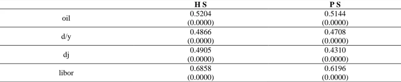
Table 2. Scaling Analysis Results Of The Robust Models
H S P S oil 0.5204 (0.0000) 0.5144 (0.0000) d/y 0.4866 (0.0000) 0.4708 (0.0000) dj 0.4905 (0.0000) 0.4310 (0.0000) libor 0.6858 (0.0000) 0.6196 (0.0000)
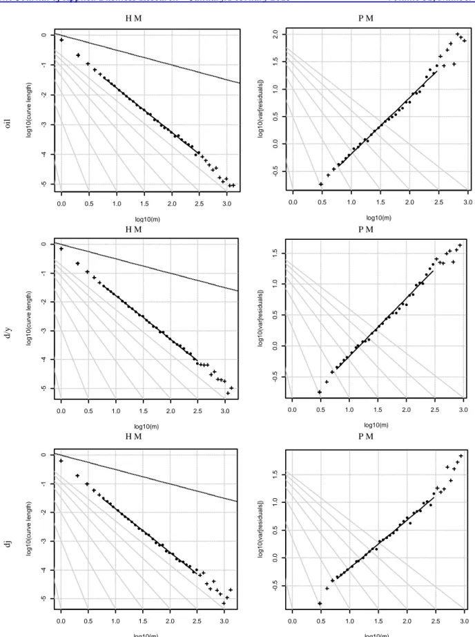
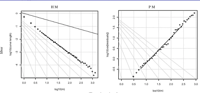
According to Table 2, the scaling exponent results exhibit a high persistency for the returns of both oil and lbr data in the 99% confidence interval. It means that both oil and lbr returns have long memory features. However, it is clear that except for lbr data, the findings of other return series are close to 0.5 from both sides. Although it is not very strong, there are short memory features in the d/y and dj data. On the other hand, as the 0.5 value of the scaling exponent also indicates the efficiency of the market, we can say that apart from the lbr data, markets related to other data appear quite efficient. The plots of the slope of scaling exponent can be seen from Figure 1.
The Journal of Applied Business Research – January/February 2015 Volume 31, Number 1 H M P M o il H M P M d /y H M P M dj
Figure 1. Scaling Exponent Plots For Robust Models
0.0 0.5 1.0 1.5 2.0 2.5 3.0 -5 -4 -3 -2 -1 0 log10(m) lo g 1 0 (cu rve l e n g th ) Higuchi Method H = 0.5205 0.0 0.5 1.0 1.5 2.0 2.5 3.0 -0 .5 0 .0 0 .5 1 .0 1 .5 2 .0 log10(m) lo g 1 0 (va r[ re si d u a ls] ) Peng Method H = 0.5145 0.0 0.5 1.0 1.5 2.0 2.5 3.0 -5 -4 -3 -2 -1 0 log10(m) lo g 1 0 (cu rve l e n g th ) Higuchi Method H = 0.4866 0.0 0.5 1.0 1.5 2.0 2.5 3.0 -0 .5 0 .0 0 .5 1 .0 1 .5 log10(m) lo g 1 0 (va r[ re si d u a ls] ) Peng Method H = 0.4708 0.0 0.5 1.0 1.5 2.0 2.5 3.0 -5 -4 -3 -2 -1 0 log10(m) lo g 1 0 (cu rve l e n g th ) Higuchi Method H = 0.4905 0.0 0.5 1.0 1.5 2.0 2.5 3.0 -0 .5 0 .0 0 .5 1 .0 1 .5 log10(m) lo g 1 0 (va r[ re si d u a ls] ) Peng Method H = 0.4311
The Journal of Applied Business Research – January/February 2015 Volume 31, Number 1 H M P M li b o r (Figure 1 continued)
4.2. Power-Law Analysis Of The Distributions
Nolan (2003) stated that heavy tails which are seen in the probability distributions of financial asset returns, perform power law behaviors. Apart from the which originates under normal distribution and has light tails, the situation which appears in the stable distributions is a sign of the power law. In these cases, the tail of the distribution decays in accordance with power law behaviors and is thicker than the normal distribution. In this study, we have used two different methods in the estimation of the parameters of the alpha-stable distribution: Ecf and Percentile. Ecf fits the parameters of the stable distribution to the empirical characteristic function estimated from the data, whereas percentile does this by using various percentiles of the data. As it can be seen from the results in Table 3, the values that are the index of the thickness of tails are between in both Ecf and Percentile methods, meaning that the type of the distribution for all of the data we have used is not normal but stable. Nevertheless, we have seen that our estimated values for d/y data are higher than the results of Borak et al. (2005), whereas the results of the d/j data is lower than both Borak et al. (2005), and Belov et al. (2006). Weron (2001) demonstrated that lower values mean thicker tails in the probability distribution. In the Gaussian distributions ( =2) tails decays more rapidly. From this point of view, we have seen that the thickest tails belong to the lbr distribution. The heaviest tails arise in the lbr, dj, oil and d/y data, respectively. On the other hand, any non-integer value between 1 and 2 demonstrates the statistical self-similarity. Accordingly, it is seen that there is self-similarity, long memory and thus fractality features in the returns.
Table 3. Estimation of the Alpha-Stable Distribution Parameters
Method data Alpha Beta Gamma Delta
Ecf oil 1.6905 -0.1126 0.0051 0.0001 d/y 1.7378 -0.1249 0.0016 -0.0000 dj 1.4119 -0.1844 0.0021 -0.0001 libor 1.1005 -0.1379 0.0015 -0.0013 Percentile oil 1.5624 -0.0685 0.0047 -0.0001 d/y 1.6222 -0.1175 0.0015 -0.0001 dj 1.3634 -0.0877 0.0020 -0.0001 libor 1.1546 -0.0826 0.0015 -0.0005
Another significant finding concerns the skewness of the distributions. As it was stated before, for the , the shape of the distribution is skewed towards the left, and the distribution is clustered in the lower values. It means that the frequency of the positive returns is higher than the negative returns. Similar to the findings of Borak et al. (2005) concerning the Dow Jones Index and Dollar/Yen currency returns, the distribution shapes of our results are all skewed to the left, as well. While this situation is valid for all of the data, the highest skewness value is seen
0.0 0.5 1.0 1.5 2.0 2.5 3.0 -4 -3 -2 -1 0 log10(m) lo g 1 0 (cu rve l e n g th ) Higuchi Method H = 0.6858 0.0 0.5 1.0 1.5 2.0 2.5 3.0 -0 .5 0 .0 0 .5 1 .0 1 .5 2 .0 log10(m) lo g 1 0 (va r[ re si d u a ls] ) Peng Method H = 0.6197
The Journal of Applied Business Research – January/February 2015 Volume 31, Number 1 in the dj data in the Ecf method and d/y data in the Percentile method. In order to estimate the statistical credibility of the obtained results, we calculated the goodness of fit statistics for all of the data. Here the hypothesis states that the data comes from the alpha-stable distribution.
Table 4. Anderson-Darling (A-D) And Kolmogorov-Smirnov (K-S) Test Results
Method oil d/y dj libor
A-D 3.0047 3.2059 3.0581 8.7954
K-S 1.7632 1.6127 1.2565 3.9019
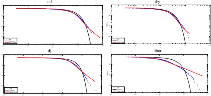
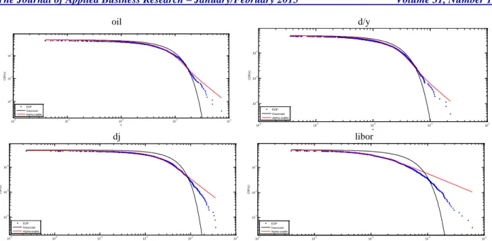
According to the results in Table 4, the test statistics of both methods reject the null hypothesis, which asserts that the data comes from an unstable distribution, in the 95% confidence interval. Figure 2 and Figure 3 represent the right and left tails of the return series for empirical distribution, normal distribution and alpha-stable distribution. In the plots, deviations of the empirical distributions from the normal distribution appear clearly. When we combine all these results with A-D and K-S test statistics, it can be seen that the alpha-stable distribution fits to all of the return series that we used.
oil d/y
dj libor
Figure 2. Right Tails Of Empirical, Alpha-Stable And Normal Distribution
10-5 10-4 10-3 10-2 10-1 10-3 10-2 10-1 100 x 1 -C D F (x ) EDF Gaussian Alpha-stable 10-5 10-4 10-3 10-2 10-1 10-3 10-2 10-1 x 1 -C D F (x ) EDF Gaussian Alpha-stable 10-6 10-5 10-4 10-3 10-2 10-1 10-3 10-2 10-1 100 x 1 -C D F (x ) EDF Gaussian Alpha-stable 10-5 10-4 10-3 10-2 10-1 10-3 10-2 10-1 x 1 -C D F (x ) EDF Gaussian Alpha-stable
The Journal of Applied Business Research – January/February 2015 Volume 31, Number 1
oil d/y
dj libor
Figure 3. Left Tails Of Empirical, Alpha-Stable And Normal Distribution
5. CONCLUSION
In conjunction with the attainability of high frequency data, new stylized facts were revealed in the financial time series; one of them is heavy tails, which states that the tails of the probability distributions decay with power law behavior, and they are thicker than the normal distribution. Another important stylized fact is the scaling property that is the hyperbolic decay in the autocorrelation functions of returns or the long memory. In this study, we researched these two stylized facts for the stock, commodity, interest, and currency markets. In the analysis of scaling properties of returns, first, eight different scaling exponent models were performed over the simulated time series for , and in order to determine the robustness of the models. The results showed that the most robust models were Higuchi’s Fractal Dimension and Peng’s Statistic as the other models’ estimated values were quite different from the control values, 0.25, 0.50 and 0.75. Therefore, we analyzed the scaling properties of the returns of the Brent crude oil, dollar/yen currency rate, Dow-Jones index and 12-month libor using these two methods. According to the results, there was high persistency in the returns of libor, and relatively lower persistency in the oil returns, whereas there were no power law features in the dollar/yen currency rate or Dow-Jones index returns. In the second part of the empirical section, we examined the power law behaviors of the tails of the probability distributions of the return series via alpha-stable distribution parameter estimations. Ecf and Percentile models results showed that values of the two models are in the range of , meaning that the tails perform power law features and are quite thicker than the normal distribution. Another considerable finding is the thickness order of the return series. Accordingly, the thickest tails belong to 12-month libor data, whereas the d/y data’s tail thickness is the lowest one. In short, in terms of the scaling properties of returns and the tail thicknesses of the probability distribution, the highest power law features were displayed in the returns of the 12-month libor data.
AUTHOR INFORMATION
Samet Günay is currently Assistant Professor of Finance at Istanbul Arel University, Turkey in the Finance and Banking Program. He has been at National University of Singapore as visiting PhD student in 2013 and at Indiana State University, USA, in 2014 as visiting scholar. His major is in finance and research interest focuses on fractals and financial econometrics. He received his BS from the Uludag University, MA from the Anadolu University and Ph.D. from Istanbul University. E-mail: [email protected]
10-5 10-4 10-3 10-2 10-1 10-3 10-2 10-1 -x C D F (x ) EDF Gaussian Alpha-stable 10-5 10-4 10-3 10-2 10-1 10-3 10-2 10-1 -x C D F (x ) EDF Gaussian Alpha-stable 10-6 10-5 10-4 10-3 10-2 10-1 10-3 10-2 10-1 -x C D F (x ) EDF Gaussian Alpha-stable 10-5 10-4 10-3 10-2 10-1 10-3 10-2 10-1 -x C D F (x ) EDF Gaussian Alpha-stable
The Journal of Applied Business Research – January/February 2015 Volume 31, Number 1 REFERENCES
1. Abry, P. & Veitch, D. (1998). Wavelet analysis of long-range-dependent traffic. IEEE Transactions on Information Theory, 44(1), 2–15.
2. Bachelier, L. (1900). Théorie de la speculation, Annales Scientifiques de L’École Normale Supérieure, 17, 21 – 86. (English translation by A. J. Boness in Cootner, P.H. (Editor), (1964), The random character of stock market prices, Cambridge, MA: MIT Press, 17 – 75.
3. Beran, J. (1994). Statistics for Long-memory Processes. Florida: CRC Press.
4. Belovas, I., Kabasinskas, A. & Sakalauskas, L. (2006). A study of stable models of stock markets. Information technology and control, 35 (1), 34-56.
5. Blattberg, R. C. & Gonedes, N. J. (1974). A comparison of the stable and student distributions as statistical models for stock prices. Journal of Business, 47, 244–280.
6. Borak, S., Härdle, W. K. & Weron R. (2005). Stable distributions. SFB 649 discussion paper, 2005-008, 1-29
7. Carr, P., Geman, H., Madan, D. B., & Yor, M. (2002). The fine structure of asset returns: an empirical investigation. Journal of Business, 75, 305-332.
8. Carr, P., Geman, H., Madan, D. B., & Yor, M. (2003). The variance gamma (v.g.) model for share market returns. Mathematical Finance, 13, 345-382.
9. Clarkson, R. S. (2002). A Fractal Probability Distribution For Financial Risk Applications. 12th AFIR, México, 1‐ 19.
10. Cont R. (2001). Empirical properties of asset returns: stylized facts and statistical issues. Quantitative Finance, 1, 223–236.
11. Fama E.F. (1963). Mandelbrot and the Stable Paretian Hypothesis. The Journal of Business, 36 (4), 420-429.
12. Fama, E. F. (1965). Random walks in stock prices. Financial Analysts Journal, 21 (5), 55-59. 13. Fama, E.F. & Roll, R. (1971). Parameter etimates for symmetric stable distributions. Journal of the
American Statistical Association, 66, 331-338.
14. Geweke, J. & Porter-Hudak, S. (1983). The estimation and application of long memory time series models. Journal of Time Series Analysis, 4(4), 221–238.
15. Hassler, U. (1993). Regression of spectral estimators with fractionally integrated time series. Journal of Time Series Analysis, 14(4), 369–380.
16. Higuchi, T. (1998). Approach to an irregular time series on the basis of the fractal theory. Physica D: Nonlinear Phenomena, 31(2), 277–283.
17. Kim Y. S., Rachev S. T., Bianchi M. L., & Fabozzi F.J. (2008). Financial market models with Le´vy processes and time-varying volatility. Journal of Banking & Finance, 32, 1363–1378.
18. Kim Y. S., Rachev S. T. Bianchi M.L., Mitov I. & Fabozzi F.J. (2011). Time series analysis for financial market meltdowns. Journal of Banking & Finance, 35, 1879–1891.
19. Levy, P. (1925). Calcul des Probabilites, Gauthier Villars.
20. Liu Y., Gopikrishnan P., Cizeau P., Meyer M., Peng C.K. & Stanley H.E. (1999). Statistical properties of the volatility of price fluctuations. Physical Review E, Vol.60 (2), 1390-1400.
21. Lo, A.W. (2000). Finance: A Selective Survey, Journal of the American Statistical Association. 95 (450), 629-635.
22. Mandelbrot B. B. & Hudson R. L. (2004), The Misbehavior of Markets: A Fractal View of Financial Turbulence, New York: Basic Books.
23. Mandelbrot, B. B. (1963). The variation of certain speculative prices. Journal of Business, 36, 392–417. 24. Mandelbrot B. B., & Wallis J. R. (1968). Noah, Joseph, and Operational Hydrology. Water Resour. Res., 4,
909–918.
25. Mantegna, R.N. & Stanley, H. E. (1995). Scaling behavior in the dynamics of an economic index. Nature, 376, 46 – 49.
26. McCulloch, J. H. (1986). Simple consistent estimators of stable distribution parameters. Communications in Statistics, Simulations, 15(4), 1109-1136.
27. Mittnik S., Doganoglu T. & Chenyao D. (1999). Computing the probability density function of the stable paretian distribution. Mathematical and Computer Modelling, 29, 235-240.
The Journal of Applied Business Research – January/February 2015 Volume 31, Number 1 28. Nolan, J. P. (1999). An algorithm for evaluating stable densities in Zolotarev's (M) parametrization.
Mathematical and Computer Modelling, 29, 229-233.
29. Nolan J. P. (2001). Maximum Likelihood Estimation and Diagnostics for Stable Distributions. Lévy Processes, Theory and Applications, 379-400.
30. Nolan J. P. (2003). Modeling financial data with stable distributions, Handbook of heavily tailed distrutions in finance. Amsterdam: Elsevier.
31. Pareto, V. (1897). Cours d Economic Politique. 2, Paris: F.Pichou.
32. Peters, E.E. (1996). Chaos and Order in the Capital Markets: A New View of Cycles, Prices, and Market Volatility, Usa: John Wiley&Sons.
33. Plerou V., Gopikrishnan P., Amaral L.A.N., Meyer M., and Stanley H.E. (1999). Scaling of the distribution of price fluctuations of individual companies. Physical Review E, 60 (6), 6519-6529.
34. Samorodnitsky, G. & Taqqu, M. S. (1994). Stable Non-Gaussian Random Processes, New York: Chapman & Hall.
35. Sheng, H. & Chen, Y.Q. (2010). Tracking performance of Hurst estimators for multifractional Gaussian processes. 4th IFAC Workshop on Fractional Differentiation and Its Applications, Badajoz, Spain. 36. Taqqu, M., Teverovsky, V. & Willinger, W. (1995). Estimators for long-range dependence: an empirical
study. Fractals, 3, 785-798.
37. Taqqu, M.S. & Teverovsky, V. (1998). On estimating the intensity of long-range dependence in finite and infinite variance time series. (Editors: Adler R., Feldman R., and Taqqu M., A Practical Guide To Heavy Tails: Statistical Techniques and Applications), 177–217.
38. Sun W., Rachev S. & Fabozzi, F. J. (2007). Fractals or I.I.D.: Evidence of Long-Range Dependence and Heavy Tailedness from Modeling German Equity Market Volatility. Journal of Economics and Business, 59 (6), 575-595.
39. Weron R. (2001). Levy-stable distributions revisited: tail index > 2 does not exclude the Levy-stable regime. International Journal of Modern Physics C, 12 (2), 209-223.
40. Weron R. (2002). Estimating long-range dependence: Finite sample properties and confidence intervals. Physica A, 312, 285 – 299.
41. Ye X., Xia X., Zhang J. & Chen Y. (2012). Effects of trends and seasonalities on robustness of the Hurst parameter estimators. IET Signal Processing, 6 (9), 849–856.
The Journal of Applied Business Research – January/February 2015 Volume 31, Number 1 NOTES