THE REPUBLIC OF TURKEY
BAHCESEHIR UNIVERSITY
IMAGE SEGMENTATION AND TEXTURE MAPPING
ON PILLOWS USING FULLY CONVOLUTIONAL
NEURAL NETWORKS
Master’s ThesisEfe Çağın KAPTAN
THE REPUBLIC OF TURKEY
BAHCESEHIR UNIVERSITY
THE GRADUATE SCHOOL OF NATURAL AND
APPLIED SCIENCES
COMPUTER ENGINEERING
IMAGE SEGMENTATION AND TEXTURE
MAPPING ON PILLOWS USING FULLY
CONVOLUTIONAL NEURAL NETWORKS
Master’s Thesis
Efe Çağın KAPTAN
ADVISOR: Asst. Prof. Dr. Tarkan AYDIN
ACKNOWLEDGEMENTS
I want to thank Asst. Prof. Dr. Tarkan AYDIN for being an amazing supervisor for my thesis. I benefited very much from his knowledge and suggestions during my research period.
Furthermore, I would like to thank my wife and my family for their patience and never-ending support.
iv ABSTRACT
IMAGE SEGMENTATION AND TEXTURE MAPPING ON PILLOWS USING FULLY CONVOLUTIONAL NEURAL NETWORKS
Efe Çağın KAPTAN Computer Engineering
Thesis Supervisor: Asst. Prof. Dr. Tarkan AYDIN
January 2018, 48 Pages
In this work, an autonomous texture mapping framework implemented that does not require a 3D model of an object. Under this framework, we combine two main tasks such as “Image Segmentation” and “Texture Mapping” into a unique architecture that runs automatically without human interaction.
The first goal of this thesis is to implement and evaluate a deep neural network (fully convolutional neural network) for the segmentation of an apparel object. Generating a quadrilateral grid on the texture area is the second step after segmentation. As the computation is faster and without 3D model requirements, this technique can be easily applied to internet applications to visualize apparel products such as pillows, sofas etc. Our goal is combining state-of-the-art deep learning architectures with texture mapping technique in an autonomous way.
Our final results have proven that our system can be a good showcase for the final appearance of clothing and apparel products inside of interior spaces.
v ÖZET
KONVOLUSYONAL AĞLAR ILE GÖRÜNTÜ SINIFLANDIRMA VE DOKU GİYDİRME
Efe Çağın KAPTAN Bilgisayar Mühendisliği
Tez Danışmanı: Asst. Prof. Dr. Tarkan AYDIN
Ocak 2018, 48 Sayfa
Bu çalışmadaki temel amaç, herhangi bir 3D modele ihtiyaç duymadan otomatik çalışan görsel tabanlı doku giydirme gerçekleştirmektir. Görüntü sınıflandırma ve doku giydirme tekniklerini tek bir çatı altında toplayarak, insan faktörü olmadan çalışan bir mimari oluşturulmuştur.
Çalışmadaki ilk hedef, görselin derin öğrenme yöntemi ile sınıflandırılmasıdır. Giydirmenin efektif olması için tekstil dokusuna sahip olan nesneler seçilmiştir. İkinci adım ise bölütlenmiş obje alanına doku ızgarası oluşturup, ardından örnek bir dokunun giydirilmesidir. Bilimsel hesaplamanın hızlı olması ve 3D modele ihtiyaç duyulmaması nedeni ile uygulanan yöntemin farklı uygulama alanları bulunmaktadır. Bir yastığın veya koltuğun farklı kumaşlar ile tanıtımını amaçlayan bir internet uygulaması kolayca gerçekleşebilecektir. Çalışmadaki temel amaç, derin öğrenme alanındaki en yeni güncel teknolojileri, doku giydirme teknikleri ile harmanlayabilmektir. Simülasyon örnekleri göstermiştir ki, çalışmada kullanılan teknik, kumaş kaplamada ve iç mimari tanıtımında faydalı olabilecektir.
vi CONTENTS TABLES ... vii FIGURES ... viii ABBREVIATIONS ... x 1. INTRODUCTION ... 1 2. GENERAL INFORMATION ... 3 2.1 DEEP LEARNING ... 3 2.2 IMAGE SEGMENTATION ... 5
2.3 CONVOLUTIONAL NEURAL NETWORK ... 6
2.3.1 Feed-Forward Neural Networks ... 7
2.3.2 Convolutional Neural Networks ... 15
2.3.3 Fully Convolutional Neural Networks ... 18
2.4 TEXTURE MAPPING ... 21
2.4.1 Bilinear Interpolation ... 22
3. METHODOLOGY ... 25
3.1 IMAGE SEGMENTATION ... 26
3.1.1 Preparing Training Data ... 26
3.1.2 Neural Network Consideration ... 28
3.1.3 Segmentation Using FCNN ... 29
3.1.4 Training And Evaluation ... 30
3.2 GRID GENERATION ... 38 3.3 TEXTURE MAPPING ... 42 4. SIMULATION EXAMPLES ... 44 5. CONCLUSION ... 48 REFERENCES ... 49 CURRICULUM VITAE ... 53
vii TABLES
Table 3.1 : Distribution of ground-truth data for training ... 27
Table 3.2 : Validation performance - MaxF1 (Raw) ... 34
Table 3.3 : Validation performance – Average Precision (Raw) ... 34
Table 3.4 : Validation performance – MaxF1 (Smooth) ... 35
viii FIGURES
Figure 2.1 : Visualizing a 3 layer deep neural network architecture ... 4
Figure 2.2 : Architecture of a convolutional neural network ... 5
Figure 2.3 : An example of feed-forward neural network ... 9
Figure 2.4 : Demonstration of dropout technique in a neural network ... 14
Figure 2.5 : Visualization of exemplary filter responses taken from a CNN ... 16
Figure 2.6 : This example demonstrates the effect of max and average pooling ... 17
Figure 2.7 : A Fully Convolutional Neural Network (FCNN) ... 19
Figure 2.8 : Classification at image-level versus pixel-level ... 20
Figure 2.9 : This figure illustrates the "skip" architecture ... 21
Figure 2.10 : Bilinear interpolation ... 23
Figure 2.11 : Example of bilinear interpolation operation on a quadrilateral grid ... 24
Figure 3.1 : Demonstration of main steps of architecture that built for this work ... 25
Figure 3.2 : Overview of ground-truth images that aligned together ... 26
Figure 3.3 : Utilization of the our training dataset ... 27
Figure 3.4 : Illustration of the VGG16 net-architecture ... 29
Figure 3.5 : Representation of the FCNN that was used in this work ... 30
Figure 3.6 : Segmentation result of VGG network with pretrained model ... 31
Figure 3.7 : Logs of our training after six hours on NVIDIA TESLA GPU... 32
Figure 3.8 : Evaluation samples after training for six hours in our FCNN ... 36
Figure 3.9 : Evaluation samples of our fully convolutional neural network ... 37
Figure 3.10 : FAST corner detection simulation for a segmentation result ... 38
Figure 3.11 : Generated 10x10 grid on segmented object ... 39
Figure 3.12 : Generated final grid with parameters rows=50 and columns=50 ... 41
ix
Figure 3.14 : Mapping a sample seamless texture image to calculated grid ... 43
Figure 3.15 : Combining final texture with original cropped image. ... 43
Figure 4.1 : Simulation of texture mapping after segmentation ... 44
Figure 4.2 : Simulation of texture mapping after segmentation ... 45
Figure 4.3 : A sample of texture mapping implementation after segmentation ... 46
x
ABBREVIATIONS
2D : 2 Dimensional
3D : 3 Dimensional
CNN : Convolutional Neural Network
FAST : Features from Accelerated Segment Test
FCNN : Fully Convolutional Neural Network
GPU : Graphics Processing Unit
PRELU : Parametric Rectified Linear Units
RELU : Rectified Linear Units
1. INTRODUCTION
As with advances in computer graphics, realistic computer-generated images have been implemented by texture mapping applications. In most cases, texture mapping algorithms focus on the connection between a 2D image and a 3D model of an object. In this context, there is a corresponding pixel on the target area at each point on the 3D model. Many of these previous algorithms require a 3D model and panoramic images. Therefore, these texture mapping algorithms are greatly limited. For example, 3D model-based texture mapping can not be processed in modern web-based applications as the main problem is such big size models can’t be streamed through the network. Moreover, it is not an easy task to build an object’s 3D model for a novice.
In this article, one of the main motivations is the use of texture mapping without the need for a 3D model of the object. In recent years, the study of computer vision addressed the problem of automating the detection and segmentation of an object on a 2D image. Semantic segmentation is an important step in understanding the object. The goal is to automatically segment an object in a particular image. Machine learning techniques have been successful in this area, especially in recent years. The state of the art in the automating visual segmentation is seen in the deep learning research community. The research on machine learning focuses on the idea that a computer can get the ability to learn just like a person without sending commands on how to proceed. Deep learning is one of the areas of machine learning and refers to the application of a set of algorithms called neural networks, and their variants. The development of larger, faster and cheaper computing units (GPU’s) has led to a revival of deep learning techniques. Deep Learning has proven itself in many areas. New architectures, algorithms and tools were developed in a short time.
Given this information on this context, implementation of a deep neural network (fully convolutional neural network) is the first objective of the segmentation of an apparel object. The second objective is to create an interactive quadriliteral grid to associate with the texture area. The computation is faster and without a requirement of a 3D model, this technique can be easily applied to an internet application to visualize of clothing products such as
2
pillows, sofas etc. Our goal is to combine state-of-the-art deep learning architectures with texture mapping technique in an autonomous way.
3
2. GENERAL INFORMATION
This chapter builds the theoretical part of my work and provides information about state-of-the-art research. The sub-topics are organized in a consecutive order. First, I explain the concepts of deep learning and continue with the topic of image segmentation. Then I describe neural networks in general and introduce subsequently more specialized networks. Moreover, the main ideas of Fully Convolutional Neural Networks which play an important role for this work, are explained. Furthermore, I will introduce the texture mapping techniques that are fundemantal for simulation in this work.
2.1 DEEP LEARNING
The history of neural networks goes back far into the past. In the mid-1980s, the first deep neural networks were applied to recognition tasks. Although this was a scientific success, the interest continued to decrease as the training took too much time. After many years, the development of larger, faster and cheaper IT units has revived deep learning techniques. Deep Learning has been used successfully in many areas. New architectures, algorithms and tools are created in a short time.
Artificial neural networks were described as the composition of simple and interconnected units that change their state according to external inputs [6].
4
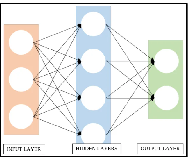
Figure 2.1 : Visualizing a 3 layer deep neural network architecture.
Source : Karpathy Andrej. Convolutional Neural Networks for Visual Recognition (Course Notes).
Neural networks can generally be identified by neurons within a human brain. The design of the neural networks is similar to a layered architecture that each layer follows each other. In this system, ever layer consists of several units (or neurons) and preceding activation functions such as sigmoid or relu which we will describe in more detail in the following chapters. A very basic level deep learning architecture shown in Figure 2.1 Deep neural networks can be considered as self-learning mechanisms. The principle of this learning path is to extract features. Auto learned features exist in the deep layers of networks. By analyzing the pixels of an image, we get learned features that are the basics functionality of common tasks such as semantic segmentation, object detection, and so on.
These parameters of the model (ie. the neurons inside hidden layers in Figure 2.1) for instance, is a classical optimization problem where parameters trained and updated
5
several times. In our learning process, ground-truth labels act as the source for our training loops. A cost function calculates a cost value that should be as low as possible during training process. Depending on the cost value, the parameters inside hidden layers should be updated through the system. Changing parameters (weights, biases) in the deep neural network usually done via gradient descent or stochastic gradient descent methods. The entire optimization process during training is called “backpropagation algorithm”.
Figure 2.2 : Architecture of a convolutional neural network.
Source : Karpathy Andrej. Convolutional Neural Networks for Visual Recognition (Course Notes).
Figure 2.2 shows a deconvolution network proposed in [30]. We can see the gradual progress of (de)convolutional layers and (un)pooling layers (functions) across the network.
The layers of a neural network can be of different types: convolutions that consist of filters, pooling layers which introduce a translational invariance to the network, and more. Figure 2.2 shows a visualization of such a convolutional neural network.
2.2 IMAGE SEGMENTATION
Pixel-level information of an image has been analyzed in different ways over the years, but the fundamental principles remain the same: identify objects in images and access their importance [7]. The problem of learning from visual information is generally classified into image classification [33], object localization and detection [14], semantic segmentation and instance segmentation [37] and the others [19].
6
Semantic segmentation can be understood as classification process of every pixel in a picture. The terms “scene analysis” or “image analysis” are often used in the same context in the literature. The remainder of this section details recent advances in dealing with the image segmentation problem, along with literature survey.
State-of-the-art networks (or models) in this space are obtained by evaluating performance on large scale benchmark datasets, such as the Microsoft Common Objects in Context (MSCOCO) [23], ImageNet [32] and PASCAL VOC [8]. MSCOCO is a famous dataset that consists of classified, segmented and labelled data with more than 300.000 images and 80 object categories, while ImageNet is a large scale dataset with more than 14.000.000 images and more than 1000 categories, with different subsets used for each benchmark task.
Most state-of-the-art results were designed for the image classification task, wherein an object class is assigned to an image as a whole. [24] presented a modified version of VGGNet [33] - which originally took in images of a constant shape to classify them amongst a large group of classes. The VGGNet model itself improved upon previous image classification networks, notably AlexNet [21], by getting rid of local response normalization layers. The power of VGGNet also lay in its simplicity, with a very homogeneous structure as compared to previous models. The models introduced in [24], referred to as Fully Convolutional Neural Networks (FCNN) modified the original VGGNet designed for an image classification task, for the image segmentation task.
2.3 CONVOLUTIONAL NEURAL NETWORKS
The conventional approach to solving a classification/segmentation problem is to decompose it into at least two independent subtasks such as feature extraction and classification. The process of feature extraction can be very complex, typically requires domain expertise and a lot of development time. A popular example for a hand-crafted visual feature is SIFT (“scale-invariant feature transform”) [26] developed by David Lowe. Lowe has put a lot of effort in the development of a feature that does not change when you rotate and scale images. SIFT has been used successfully for object recognition or panorama stitching tasks.
7
The downside is that these features are very rigid and do not automatically adapt to the problem. The classification step however has always been a machine learning approach. Based on the extracted features, any appropriate classification algorithm can be applied (e.g. a support vector machine).
An alternative approach is to integrate both feature extraction and classification into one learning process. Since the features are learned automatically, expert domain knowledge and time-consuming engineering are not required. Furthermore, it is possible to train feature extraction and classification in an end-to-end manner, which allows a better optimization and adaption of both parts.
This work uses a special convolutional neural network (CNN), which extracts features and classifies the input image pixel-wise for image segmentation. For the sake of a step-wise introduction, we first introduce feed-forward neural networks and explain the basic concepts of neural networks.
2.3.1 Feed-forward Neural Networks
Feed-forward networks are collections of neurons, which are organized in layers 1, ..., L. Every neuron of layer 𝑙 > 1 connects to every neuron of the previous layer 𝑙 − 1. When deployed a feed-forward net has a distinct direction ("forward pass") and there are no cycles (feedback loops). The layers are distinguished between input, output and hidden layers. Hidden layers are placed between the input and output layer and therefore do not have a direct connection to the environment.
The special case where the network consists of only two layers (in- and output) is called single-layer perceptron. Since the input layer is not parameterized, it is frequently not considered as a layer. For this reason, it is called single-layer perceptron. More usual are the so called multi-layer perceptrons, where several layers are put together on top of each other. Thus, such a multi-layer perceptron has at least one hidden layer.
Figure 2.3 shows a basic network with an input, output and a hidden layer. Each connection between two neurons 𝑖 and 𝑗 is associated with a weight 𝑤𝑗,𝑖(1). The superscript 𝑙 denotes the number of the layer. These weights are used to calculate a
8
weighted sum of all 𝐽 inputs. In general there are also bias-terms 𝑏𝑖(1) associated to each neuron. This bias term shifts the weighted sum by a certain amount.
This intermediate result is then processed by a so-called activation function ℎ. Usually this function applies a non-linear transformation. The result is the output of the neuron and possibly serves as input for the next layer (if layer 𝑙 is a hidden layer). The below equation shows the formula for calculating the activation 𝑎𝑖𝑙 of a specific neuron located at position 𝑖 in layer 𝑙 for 𝐽 inputs 𝑥𝑗 :
𝑎𝑖 𝑙 = ℎ(𝑏𝑖𝑙+ ∑ 𝑤𝑗,𝑖𝑙 . 𝑥𝑗 𝑗
𝑗=1
)
where:
𝑎𝑖𝑙 is the activation of neuron 𝑖 at layer 𝑙
ℎ(𝑥) is the activation function
𝑤𝑗,𝑖𝑙 is the weight of neuron 𝑖 at layer 𝑙 associated with input neuron 𝑗
𝑏 is the bias of neuron 𝑖 at layer 𝑙 𝑥𝑗 input (result of neuron 𝑗 when 𝑙 > 1)
Typical activation functions are the sigmoid (logistic) or the hyperbolic tangent function. In this work so-called rectified linear units (ReLU) were used:
ℎ𝑅𝑒𝐿𝑈(𝑥) = max (0, 𝑥)
ReLUs employ a simple ramp function and are crucial for the success of recent deep networks [21]. [33].
9
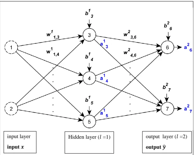
Figure 2.3 : An example of feed-forward neural network
Source : Hinton G. E., Srivastava N., Krizhevsky A., Sutskever I and Salakhutdinov R. R., “Improving
neural networks by preventing co-adaptation of feature detectors,” July 2012
An example of feed-forward network consists of one input, one output and one hidden layer shown in Figure 2.3. The neurons, visualized by solid circles, are organized in layers 𝑙. Each connection between two neurons is associated with a (learned) weight 𝑤𝑗,𝑖𝑙 . The weighted sum of the input values plus a bias term 𝑏𝑖𝑙 is then fed into an activation function, which results in the activation 𝑎𝑖𝑙. The values are propagated throughout the entire network. Finally, the output layer is reached which produces the net output 𝑦̂.
A neural network is entirely defined by its structure (topology), the activation functions and its parameters (namely weights and biases). In general a neural network can approximate any finite function [1].
To handle discrete outputs, such as it is needed for classification tasks, a probability function for each of the defined states can be trained in order to finally select the class
input layer input 𝒙
Hidden layer (𝑙 =1) output layer (𝑙 =2)
10
with the highest probability. Usually, the probabilities are obtained by applying a softmax normalization in the output layer. An exponential function 𝑒𝑥𝑝(𝑦̂𝑛, 𝑦𝑛) turns the class prediction into a non-negative value. Then this value is normalized by the denominator to fit the [0, 1] range. In this way all class probabilites sum up to 1.
𝜎𝑐 = exp (𝒚̂𝑛,𝑦𝑛) ∑𝐶𝑐=1exp (𝒚̂𝑐)
where:
C is the number of classes
𝒚̂𝑐 is the predicted class score with 𝑐 = 1,...,C
𝒚̂𝑛,𝑦𝑛 is the predicted class score of the true class 𝑦𝑛 for sample 𝑛
The parameters of a neural network are learned based on training samples. In case of supervised learning, where a labelled training set is given {(𝑥𝑛, 𝑦𝑛)}, all classifications have to be penalized by a suitable loss function 𝑙(𝑦̂𝑛,𝑦𝑛), also called cost function. This loss function must be minimized. Usually, a regularization term 𝑟 is added in order to preserve the model from overfitting. This occurs when individual parameters dominate over others. The weights should be kept as small as possible. This why the regularization term is also called "weight decay". This can be achieved by minimizing the L2 norm of the parameter vector. The balance between regularization and loss is controlled by a hyperparameter ∝. In summary the regularized error function E is as follows:
𝐸(𝜔, 𝑏) = 𝑙(𝑦̂𝑛, 𝑦𝑛) + 𝛼 . 𝑟(𝜔)
where:
𝜔 weight 𝑏 bias
𝑦𝑛 is the class label i.e. the true class
𝑦̂𝑛 is the class prediction
11
𝑟(𝜔) is the regularization term (weight decay)
A popular loss function for multi-class classification objectives is the multinomial logistic loss. Passing class probabilities 𝜎 conditioned on the input data 𝑥𝑛, the multinomial logistic loss is the true class negative log-likelihood of the 𝑦𝑛. The total loss 𝑙𝑡𝑜𝑡 of one training batch is given by the sum over all samples 𝑁. The below equation shows the normalized multinomial logistic loss 𝑙̅ which additionally includes a normalization term 1/N: 𝑙̅ = − 1 𝑁 ∑ log (𝜎𝑛,𝑦𝑛) 𝑁 𝑛=1 where:
𝑁 is the number of training samples 𝑦𝑛 is the class label i.e. the true class
𝜎𝑛𝑦𝑛 is the class probability conditioned on the input of the true class 𝑦𝑛
As previously mentioned, the training process aims to adopt the parameters such that the loss is minimized over all training samples. Thus, we search the function f parametrized by w, which minimizes the loss 𝑄(𝑥, 𝑦, 𝑤) = 𝑙( 𝑓𝑤(𝑥), 𝑦) averaged over the examples (i.e. pairs of 𝑥 and 𝑦). A standard technique for solving nonlinear optimizing problems is gradient descent [29]. Gradient descent iteratively adopts variables towards the direction of the negative gradient. This way a local minimum can be found. The learning rate 𝛾 determines the steps size of each adaptation.
𝑤𝑡+1 = 𝑤𝑡− 𝛾 1 𝑁∑ ∇𝑤 𝑁 𝑛=1 𝑄(𝑥𝑛𝑦𝑛𝑤𝑡) = 𝑤𝑡− ∆𝑤𝑡 where:
𝑤 are the weights 𝛾 is the learning rate
12
𝑄 is the loss function 𝛻𝑤 is the gradient w.r.t. w
∆𝑤𝑡 is the weight update
N number of samples
According to the equation, the weight update ∆𝑤𝑡 incorporates all training samples {(𝑥𝑖, 𝑦𝑖)}.
An abreviation of gradient descent is the stochastic gradient descent method [4]. Stochastic gradient descent shows its strengths when the training set is very large. Instead of computing the gradient based on all samples, only one or a few randomly chosen samples are considered. The updated weight 𝑤𝑡+1 in the following equation is based on a randomly chosen example 𝑥𝑡.
𝑤𝑡+1= 𝑤𝑡− 𝛾𝑡 𝑄(𝑥𝑛𝑤𝑡) = 𝑤𝑡− ∆𝑤𝑡
where:
𝑤 are the weights 𝛾 is the learning rate Q is the loss function 𝛻𝑤 is the gradient w.r.t. 𝑤
∆𝑤𝑡 is the weight update
An extension of stochastic gradient descent is momentum [29]. Momentum helps to speed up the learning process by adding a fraction m of the previous weight update.
𝑤𝑡+1 = 𝑤𝑡− (∆𝑤𝑡+ 𝑚∆𝑤𝑡−1)
where:
13
∆𝑤𝑡 is the weight update
𝑚 is the momentum parameter
If both weight updates point towards the same direction the step size is amplified. In case of changing gradients momentum smooths out the variations and provides stability. By providing training samples 𝑥 and 𝑦, a single layer perceptron can be optimized by any gradient descent variant. This is because the input and outputs of the single weight layer are known. Therefore the delta term or error 𝑦 ̂ − 𝑦 is directly computable. This is not the case for networks including hidden layers.
This fact is the motivation for applying the so-called backpropagation algorithm [29]. In order to adjust the parameters of hidden layers the error is propagated subsequentially ack through the net. This process is called backward pass. The parameter adjustment (i.e. the delta term) of layer 𝑙 depends on the activation of the same layer, the weights and the delta terms of the subsequent layer 𝑙 + 1. The activations are determined during the forward pass. In this way the partial derivatives w.r.t. the parameters of each neuron can be determined (chain rule). Gradient descent uses these delta terms for updating the parameters.
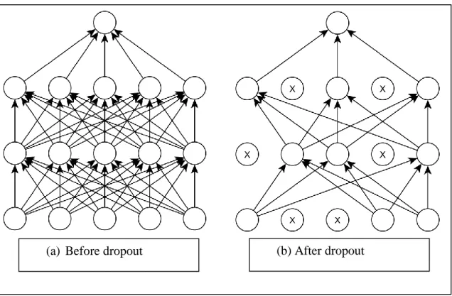
Dropout invented by Hinton et al. is another powerful regularization tool for training neural networks [17]. For each iteration dropout randomly turns off a portion of neurons (see Figure 2.4).
14
Figure 2.4: Demonstration of dropout technique in a neural network
Source : Hinton G. E., Srivastava N., Krizhevsky A., Sutskever I and Salakhutdinov R. R., “Improving
neural networks by preventing co-adaptation of feature detectors,” July 2012.
The effect of dropout applied on a simple neural network demonstrated in Figure 2.3. Dropout randomly removes a portion of connections between subsequent layers and produces a thinned network [35].
That way each hidden unit is encouraged to learn meaningful features without relying to much on other hidden units. More precisely, randomly chosen submodels are trained, thus comparable to ensemble learning. At test time the predictions are averaged. This leads to significantly better generalization [35].
Neural networks trained by the backpropagation algorithm suffer from the socalled "vanishing gradient problem" [18]. Especially for very deep networks this effect is even amplified. For example the gradient ℎ’(𝑥) of the sigmoid function ℎ(𝑥) = (1 + 𝑒𝑥𝑝(−𝑥))−1 tends towards zero as |𝑥| increases. This cumbers the learning process and limits the network size for end-to-end training. In practice this problem is attenuated by using ReLUs, careful initialization [11][15] and small learning rates.
15
Furthermore, very deep networks are usually trained step by step i.e. the size of the network is gradually increased [33].
Parametric ReLUs (PReLU) include an adjustable slope for the negative part. This slope can be controlled by a factor 𝑠𝑖.
ℎ(𝑥) = max(0, 𝑥) + 𝑠𝑖min (0, 𝑥)
where
𝑠𝑖 factor to control slope for the negative part
He et al. have recently shown that learning the PReLU parameter 𝑠𝑖 together with an improved random initialization helps end-to-end learning of large networks [15]. Another attempt for preventing the "vanishing gradient problem" was described by Ioffe and Szegedy [18]. They normalize the inputs of the activation functions such that the distribution remains stable during training.
2.3.2 Convolutional Neural Networks
In the previous section the main ideas of feed-forward networks were introduced. A Convolutional Neural Network (CNN) is a special kind of feed-forward neural network. CNNs are inspired by the biological processes of visual perception. Therefore CNNs are mainly used for image and video applications. In principal there are three extensions that distinguishes a CNN from a simple feed-forward network: weight sharing, spatial pooling and local receptive fields.
The input of a CNN is processed patch-wise by a number of learned convolutions. With the help of these convolutions various filter techniques can be applied e.g. blurring, edge or corner detection. Discrete convolutions are calculated by shifting a filter mask over the input image and calculating the sum of products. The result is written to the current center of the mask. These filter masks produce the so-called local receptive fields. Intuitively they define the image crops that a neuron actually "see". In terms of neural networks the entries of the filter masks correspond to the weights of the neurons and the filter size defines the connectivity between neurons of subsequent layers.
16
Since many filters are applied several feature maps are obtained. All neurons of a feature map share the same weight matrix. This property is called weight sharing.
Figure 2.5: Visualization of exemplary filter responses taken from a CNN that has
. three hidden layers. Each filter responds differently to the input.
Source : Zeiler M. D. And Fergus R., “Visualizing and understanding convolutional networks,” Nov. 2013
Weight sharing contributes to the property of shift invariance, since the same convolutions are applied to the entire input image. At the same time weight sharing reduces the amount of free parameters dramatically. This makes the net much easier to train and has a strong regularization effect.
The learned filters expose different kind of visual features. Investigations by different researchers have shown that the early layers typically capture very simple features, similar to gabor filters and color patches [40] [27]. These features are very general and therefore apply to many use-cases. In contrast the features of higher layers are more abstract and reflect the gist of the learned classes. Exemplary filter responses of an early convolutional layer are shown in figure 2.5.
17
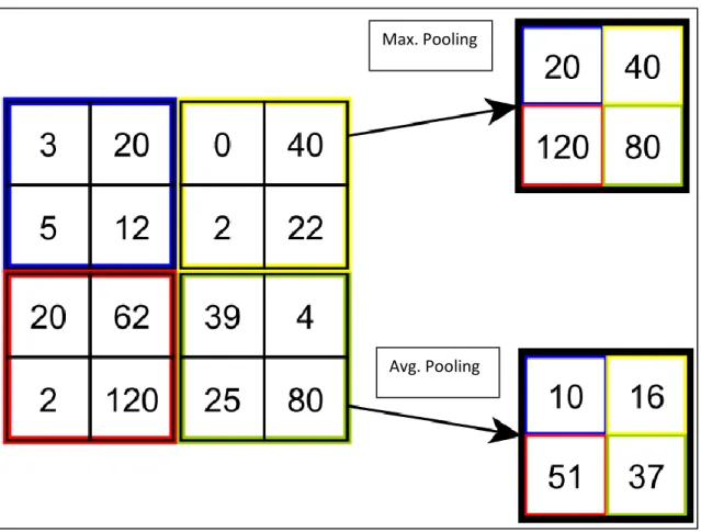
Figure 2.6: This example demonstrates the effect of max and average pooling.
Another important component of CNNs are pooling layers. Typically the data is sub-sequentially downsampled by combining spatial pools to a single value. Pooling reduces the feature space and grant a small amount of translational invariance. This is due to the fact that neurons within a region are mapped onto a single neuron. Frequently used pooling operations are avarage and maximum pooling (see Figure 2.6). A more recent method is stochastic pooling [41], which serves as an regularizer similar to dropout. So far the feature maps cover a two-dimensional space. For high-level reasoning, such as classifying an image, a one-dimensional representation is needed. This can be achieved by a fully connected layer. In fully connected layer, each neuron is connected to all neurons of the previous layer. Thus, fully connected layers aren’t spatially located anymore. The one-dimensional output, is suitable for a traditional multi-layer perceptron classifier.
Max. Pooling
18
CNNs, in recent years, became popular in image classification tasks [21] [33]. Many models are shared within the researcher community, which makes it possible to follow up and adopt the networks to other classification problems. This process is called "finetuning". Initializing from pretrained weights works well for many cases. Even a model trained on a very distant task is often a better starting point than initializing from random numbers (like "xavier" [11] or "msra" initialization [15]). One reason for this is that features of early layers are in fact very general. Yosinksi et al. investigated on the question of transferability [39]. Deep Learning Frameworks such as Caffe facilitate the transferal of learned weights.
After the great success of CNNs for image classification, the natural next step was to apply CNNs to local tasks, such as bounding box detection [10] [12] [13], local correspondence [25] or semantic segmentation [9] [10] [12] [13].
Even though the results for semantic segmentation tasks yield new record accuracies on various datasets, the methodologies had some major drawbacks. A common approach was to identify clusters in the image, which may hold the desired objects ("region proposals"). All clusters are then classified independently. The results are then merged to obtain a segmentation mask. This approach requires extensive preand post-processing, making it unsuitable for end-to-end training and includes a considerable overhead. In addition, the clustering result is likely to be suboptimal. A fully visible object may be divided into several regions.
Therefore it was a huge improvement, when Long et al. developed a new net architecture for semantic segmentation namely "Fully Convolutional Neural Networks" (FCNN) [24].
2.3.3 Fully Convolutional Neural Networks
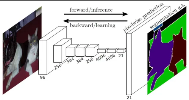
In 2014 Jonathan Long, Evan Shelhamer and Trevor Darrell published the paper "Fully Convolutional Networks for Semantic Segmentation" [24]. They presented a new neural network archiecture for pixel-wise prediction. There are several advantages compared to previous works. A FCNN processes whole-images and produces dense predictions in the form of probability maps. The training can be applied in an end-to-end behavior and densely labeled images are required for supervision.
19
Figure 2.7: A Fully Convolutional Neural Network (FCNN)
Source : Long Jonathan, Shelhamer Evan and Darrell Trevor. “Fully Convolutional Networks for Semantic
Segmentation”.
A fully convolutional neural network processes the entire image to make pixelwise predictions of the same size as the input image. The network is trained end-to-end by backpropagation and a pixel-wise loss (see Figure 2.7). This requires dense ground truths for supervised training.
Another advantage is the ability to re-interpret existing classification nets as a FCNN. Therefore a FCNN can benefit from pre-trained CNN models. In order to convert a CNN into a FCNN, we need to replace the inner layers (fully connected layers) by convolutions with a kernel size of 1x1 (see Figure 2.8).
While the fully connected layer of an image classification net completely discards spatial information and delivers only one feature vector for the entire image, the fully convolutional layer produces a feature vector for every pixel. Based on this feature map a pixel-wise classification can be performed. This yields a probability map for each class. To restore the original image dimensions this map is upsampled by so-called deconvolutions. Depending on the weights, a deconvolution can serve as a bilinear interpolation.
20
Figure 2.8: Classification at image-level versus pixel-level
Source : Long Jonathan, Shelhamer Evan and Darrell Trevor. “Fully Convolutional Networks for Semantic
Segmentation”.
In order to retain spatial information, we can "convolutionalize" a network by replacing fully connected layers by convolutions. As you can see in Figure 2.8, the main difference is fully connected layers at the end of the network.
While pooling improves classification accuracy, it partially neglects spatial information. This is a drawback as it limits the spatial accuracy of the segmentation. The VGG16- and Alex-net for example include 5 pooling layers of stride 2 [33][21]. In total this results in downsampling by factor 32 (25). In general this leads to coarse segmentation maps. Very small objects aren’t even considered at all.
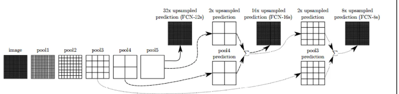
To solve this issue they use a so-called "skip" architecture (see Figure 2.9). By fusing predictions of different strides they are able to refine the segmentation maps. In addition to the classification based on the 32-stride feature map, they do the same for the outputs of earlier pooling layers and fuse the classification scores by taking the element-wise sum. Of course such an element-wise operation affords inputs of the same size. Thus, the smaller prediction maps must be interpolated accordingly.
21
Figure 2.9: This figure illustrates the "skip" architecture developed by Long et al..
Source : Long Jonathan, Shelhamer Evan and Darrell Trevor. “Fully Convolutional Networks for Semantic
Segmentation”.
To keep the net-representation compact, only pooling and classification layers are shown in Figure 2.9. All intermediate convolution layers are omitted. The coarsest prediction is based on pool5 only (solid line) and is called FCNN-32s. The FCNN-16s version (dashed line) first upsamples stride 32 predictions by a factor of 2 and then combine the output with the predictions of pool4. The FCNN-8s variant (dotted line) combines predictions of stride 32, 16 and 8.
This way they obtained new state-of-the-art results on several data-sets. However, this method left enough space for improving the spatial accuracy. Noh et al. achieve finer predictions by learning a deconvolution network [30]. The general idea is to extend a convolutional network by its mirrored counterpart. By learning the inverse operations (pooling vs. unpooling, convolution vs. deconvolution) it’s possible to produce a finer segmentation.
2.4 TEXTURE MAPPING
In the field of computer graphics, texture mapping is a common and popular technique to improve the appearance of computer generated images [16].
The main motivation is to create a map between a 3D model and a 2D image. In this plane, each point of the outer space at a pixel is connected to the original image. Declaration a parametric surface [3,5] was the purpose of previous algorithms to create that maps. The implementations of these algorithms for polygonal meshes are not
22
successful to apply texture mapping and therefore such statements are not common nowadays.
In order to find an optimal solution for this problem, we need to find a layer that it should have a simple shape. This layer will be effective for the mapping between texture area and our 3D model surface [2]. Due to the non-linearity of texture maps, these algorithms often yield high deformation results [22]. In order to obtain more efficient mapping results, a number of optimization algorithms have been developed [1,22–28,31–34,36]. A new technique has been developed by Devich and Weinhaus [38] and other researchers [20]. This technique, known as projective texture mapping, reflects the texture map (ex. a panoramic image) onto the geometry. This technique does not use a fixed texture unlike the old techniques.
In this work, we developed a texture mapping application based on images, without using 3D models. We have seen it very successful when we use this method on fabric-covered objects such as pillows or sofas. To succeed in practice, we have created an interactive texture grid on segmented objects. Texture distortion is not a problem because of the relationship between the grid and texture visual is in linear-form.
It is estimated that final result will be successful in internet or desktop applications. No requirement for a 3D model is a big reason for this conjecture. Moreover, the efficiency of computational calculation will also provide easy adaptation. In general, we foresee that this method will be used in the interior presentation of apparel products. This technique does not require any user interaction. Using the result of image segmentation, a texture mapping is done automatically which we will give details of this process in next chapter.
2.4.1 Bilinear Interpolation
Bilinear interpolation is expressed as a method of transforming a square into a quadrilateral. As can be seen in Figure 2.10, the first step of this transformation can be expressed as follows: along the bottom and top sides of the quadrilateral linearly interpolated by fraction 𝑢. The second step is linear interpolation by fraction 𝑣 between points that interpolated to form target point (𝑥, 𝑦)
23 Figure 2.10 Bilinear interpolation
(𝑥, 𝑦) = (1 − 𝑢)(1 − 𝑣)𝑝00+ 𝑢(1 − 𝑣)𝑝10+ (1 − 𝑢)𝑣10+ (1 − 𝑢)𝑣𝑝01+ 𝑢𝑣𝑝11
The matrix notation form is:
(𝑥 𝑦) = (𝑢𝑣 𝑢 𝑣 1) [ 𝑎 𝑒 𝑏 𝑓 𝑐 𝑔 𝑑 𝑓ℎ ]
The matris that contains 8 coefficients from the 4 points correlation can be computed as follows : [ 𝑎 𝑒 𝑏 𝑓 𝑐 𝑔 𝑑 ℎ ] = [ 1 −1 −1 1 −1 1 0 0 −1 0 1 0 1 0 0 0 ] [ 𝑥00 𝑦00 𝑥10 𝑦10 𝑥01 𝑦01 𝑥11 𝑦11 ]
24
Figure 2.11 : Example of bilinear interpolation operation on a quadrilateral grid.
In this chapter, we have provided background information on image segmentation and texture mapping techniques. In the next chapter, we combine these two concepts in an architecture that automatically process texture mapping after an image segmentation task.
25
3. METHODOLOGY
In this work, we design an architecture that can efficiently perform image segmentation and texture mapping simultaneously. This is done by incorporating three main tasks into a unified architecture. The first task is performing image segmentation and create a black and white mask (binary mask) image. The white colour corresponds to the object that was segmented. The second main task is to create a 2D grid (mesh) on the object. This grid is the 2D model of the segmented object. The final step is applying texture mapping with a sample texture (fabric) to the target area. We will provide detailed information on each step in the next chapters.
Figure 3.1 Demonstration of main steps of architecture that built for this work.
Figure 3.1 shows the key steps for a stand-alone texture mapping architecture of an object in the input image. The first picture is the input image that user uploads to the system. The first step is the only user interaction in the system. The second image is the output of the image segmentation process. We see the generated texture grid in the third picture after segmentation. The last picture is the final result of texture mapping of the object that was segmented automatically.
Input Image SegmentationImage Grid Generation Texture Mapping
26 3.1 IMAGE SEGMENTATION
In this chapter, we describe the deep learning framework which was used to learn the semantic segmentation of images from the new ground truth datasets, which were generated for this work.
Fully convolutional neural network (FCNN) was used as an architecture for learning semantic information. We gave detailed information of fully convolutional neural networks in chapter 2.3.3. In summary, FCNN is a neural network architecture that was implemented by Long et al. [24] in 2015. FCNN’s were proposed to model semantic segmentation using a deep learning pipeline that can be trained end-to-end.
3.1.1 Preparing Training Data
In order to process segmentation on clothing, apparel products or pillows, a custom dataset created manually. This dataset contains 250 black and white hand generated images. White colour represents the object that needs to be segmented. Figure 3.2 shows an overview of original and labelled images side by side.
27
In Figure 3.2 we see some examples of training images which prepared for this work. For each sample pillow image, a black and white ground-truth image generated by a graphics software. As we only interested in the main object, our training images consist of two colours which are black and white.
Table 3.1 Distribution of ground-truth data for training
Dataset Number of images
Training 200
Testing 25
Validation 25
Figure 3.3 : Utilization of the our training dataset.
Training = 80% Validation = 10% Testing = 10%
Training for parameter optimization
Evaluation of parameter optimization
Training for final evaluation
28
In this work, we split training data into three parts as training (%80), validation (%10) and test (10%). All datasets subsampled with random selections. This dataset is fairly small compared to common deep learning datasets. Thus the network has to transfer as much knowledge as possible from pre-training. Details of pretraining explained in next chapter.
3.1.2 Neural Network Consideration
The experiences and results of other researchers are important to find a good starting point for choosing the model architecture. Mainly based on the work of Long et al. [24] various experiments have been carried out to find a way to improve the system in general or to adapt it to certain circumstances.
Simonyan and Zisserman describe network architecture with up to 19 weight layers in their work "Very deep convolutional networks fo large-scale image recognition" [33]. The research groups of Long and Zheng used the pretrained model of the 16 layer version visualized in Figure 3.4. This network is known as "VGG16", as it was developed by Oxford’s "Visual Geometry Group" and has 16 weight layers. Figure 3.4 illustrates the topology of the network.
Characteristic for VGG-16 is an architecture that uses relatively small convolutional filters, mainly of size 3×3. These small filters result in convolutional layers with relatively few learnable parameters. This allows combining convolutional layers following each other while still yielding neural network models that can be trained in reasonable time. The VGG-16 architecture, composed of 16 layers in the ImageNet competition in 2014, achieved a very successful classification result. [32]. There are 1000 object categories in this competition.
29
Figure 3.4 Illustration of the "VGG16" net-architecture.
Source : Simonyan K. and Zisserman A., “Very deep convolutional networks for largescale
. image recognition,” Sept. 2014.
3.1.3 Segmentation Using FCNN
FCNN architecture which is used in this work is eventually based on the famous VGG-16 network [33]. Long et al. [24] transformed VGG-VGG-16 into FCNN, a fully convolutional neural network. They did so by transforming VGG-16’s fully connected layers into convolutional layers and by adding deconvolutional layers, which upsample the data back to the original input image resolution. In addition, they added three so-called "skips" to
30
the FCNN architecture, which fuse spatial information from shallow FCNN layers with semantic information from deep FCNN layers to obtain the better semantic segmentation of images. Figure 3.4 illustrates the architecture of FCNN. The name of FCNN-8s refers to the neural network layer Pool 3, which has the highest spatial resolution among those three neural network layers of FCNN-8s which are used in a "skip". Pool 3 has a spatial resolution that is roughly 8 times lower than the original input image spatial resolution. When evaluated on a PASCAL VOC 2011 subset, semantic segmentation dataset [8], FCNN achieved state-of-the art segmentation results [24]. The number of feature channels, which are used in the upper parts of FCNN, correspond to the number of different object labels, which are learned. In Long et al. [24], the number of feature channels is either 21, 33, 40 or 60 depending on the dataset which was used for learning. In FCNN, rather than producing one dimensional predictions, this leads to two-dimensional predictions i.e. the segmentation maps. In this work, the number of different object labels are always 2 (object and background).
Figure 3.5 Representation of the FCNN that was used in this work.
As shown in Figure 3.5, we take the VGG16 architecture and convert fully connected layers to 1 x 1 convulation layers to get 39 x 12 sized segmentation features. Three upsampling layers followed as a next step to produce 1248 x 384 output image with two channels. These two channels represents segmented object and background.
3.1.4 Training And Evaluation
FCNN initialized using pretrained VGG weights on ImageNet [33]. ImageNet visual recognition dataset consists of 14 million images belonging to 1000 categories. The researchers from the Oxford Visual Geometry Group, or VGG for short, made their
Input 1248x384x3 VGG16 13 Conv. Layers Encoded Features 39x12x512 FCNN 3 Upsampling Layers Prediction 1248x384x2
31
models and learned weights available online. This allowed us to use an advanced image classification model in our architecture. In Figure 3.6, we show a sample of segmentation result for a sofa object before training. “Sofa” is one of the classes of ImageNet dataset. Figure 3.6 Segmentation result of VGG network with pretrained model
32
The convolutional layers of the segmentation network initialized using VGG weights and the transposed convolution layers are initialized to perform bilinear upsampling. The skip connections, on the other hand, are initialized randomly with very small weights (i.e. std of 1𝑒 − 4). This allows us to perform training in one step (as opposed to the two step procedure of [24]).
33
Our segmentation architecture is trained with our custom dataset. This dataset is very small, providing only 200 training images. Thus the network has to transfer as much knowledge as possible from pre-training. Note that the skip connections are the only layers which are initialized randomly and thus need to be trained from start. This transfer learning approach leads to very fast convergence of the network. As shown in preceding tables, the raw scores already reach values of about 90 % after only about 4000 iterations. Training is conducted for 16.000 iterations to obtain a meaningful median score.
The segmentation performance is measured using the F1 score. The F1 score is a measurement method used for the classification in statistics field. Recall and precision values are important to calculate F1 score. Positive correct results divided by the total number of positive results equals “precision”. Positive correct results divided by positive results equals “recall”. The harmonic average of the recall and average scores defines F1 score. The worst case of the F1 score is 0 and its top/best value is 1 which we call it perfect recall and precision.
𝑝𝑟𝑒𝑐𝑖𝑠𝑖𝑜𝑛 = 𝑡𝑝
𝑡𝑝+𝑓𝑝 , 𝑟𝑒𝑐𝑎𝑙𝑙 = 𝑡𝑝 𝑡𝑝+𝑓𝑛
where:
𝑡𝑝 is the number of true positives 𝑓𝑝 is the num of false positives 𝑓𝑛 is the num of false negatives
Thus, 𝐹1 score calculated as :
𝐹1 =
2 . 𝑝𝑟𝑒𝑐𝑖𝑠𝑖𝑜𝑛 . 𝑟𝑒𝑐𝑎𝑙𝑙 𝑝𝑟𝑒𝑐𝑖𝑠𝑖𝑜𝑛 + 𝑟𝑒𝑐𝑎𝑙𝑙
In addition, the average precision score is given for reference. Classification performance is evaluated by computing accuracy and precision-recall plots.
34
Table 3.2 : Validation performance - Max F1 (Raw)
Table 3.3 : Validation performance – Average Precision (Raw)
87 88 89 90 91 92 93 94 0 2000 4000 6000 8000 10000 12000 14000 16000 18000 Va lid a tio n Sco re [ %] Iteration
Max F1 (Raw)
87,5 88 88,5 89 89,5 90 90,5 0 2000 4000 6000 8000 10000 12000 14000 16000 18000 Va lid a tio n Sco re [ %] Iteration35
In order to show result in a linear form, values smoothed using linear regression method. In Table 3.4, we show smoothed results of Max F1 score. Smoothed Avarage Precision values are shown in Table 3.5.
Table 3.4 : Validation performance – Max F1 (Smooth)
Table 3.5 : Validation performance – Avarage Precision (Smooth)
86 87 88 89 90 91 92 93 0 2000 4000 6000 8000 10000 12000 14000 16000 18000 Va lid a tio n Sco re [ %] Iteration
Max F1 (Smooth)
86 87 88 89 90 0 2000 4000 6000 8000 10000 12000 14000 16000 18000 Va lid a tio n Sco re [ %] Iteration36
Figure 3.8 Evaluation samples after training for six hours in our FCNN.
37
38 3.2. GRID GENERATION
As this work does not need any 3D model for the segmented object, a 2D grid needed for texture mapping. Before creating the texture grid, four corners of the segmented object calculated using the FAST corner detection algorithm [46].
FAST (Features from Accelerated Segment Test) has a working principle that there should be 𝑛 pixels surrounded by a corner candidate p.
Figure 3.10 : FAST corner detection simulation for a segmentation result. The pixel
. at p is a candidate corner which is at the center.
The working principle of this algorithm relies on n pixels around a candidate corner 𝑝 such that this pixel should be surrounded by n pixels that have a brighter or darker color. Surrounded pixels around corner 𝐼𝑝 are brighter if 𝑙𝑝+ 𝑡 or lighter if 𝑙𝑝− 𝑡 where 𝑡 is the threshold value. As you can see in Figure 3.8, the 𝑛 parameter is 16. When looking at points 1,5,9 and 13, it can be seen that the number 16 selected to effectively identify corner candidates. In order to estimate if p is a corner, it must be a lighter color of at least 3 points 𝑙𝑝 + 𝑡. Conversely, it should be at least 3 points 𝑙𝑝− 𝑡 darker color. If these
39
conditions are not met, this point is not considered a corner. This method applies the same comparisons to the other candidate corner points. The texture grid is calculated based on the four boundary lines which calculated by four detected corners in previous task. In first step, horizontal and vertical lines were used to calculate the texture grid.
40
In order to calculate the mesh lines with interpolation, parameters must be determined. If 𝐿𝑖 expresses a mesh line in the whole mesh, we can formulate 𝐿𝑖 as :
𝐿𝑖 = {𝑋𝑖 (𝑡) 𝑌𝑖 (𝑡)
There are 𝑛 𝐿𝑖 lines in the grid and for 𝐿𝑖 that we should calculate 𝑡 parameter on this line. Starting from the starting point of the line, we need to calculate the 𝑡 parameter for each mesh intersection. In short, we know that how many 𝑡 parameters can be calculated by dividing the line length by the number of horizontal/vertical meshes. After computing the number 𝑡, it can be seen that there are 𝑋𝑖(𝑡) and 𝑋𝑖(𝑡) coordinate points on each line. Thus, the values of 𝑡 on the line 𝐿𝑖 are computed. Since the generated grid lines are modelled completely by the segmented image, the composition of both vertical and horizontal lines are calculated. The final result will be the mesh of segmented image. Since the horizontal and vertical calculations are almost identical, we will only give information about the calculation of horizontal lines. As mentioned earlier, mesh lines are calculated by linear interpolation. During this process, weights must be formulated for each row. if the number 𝑚 is considered to represent the number of lines, the weight 𝑤𝑔1, 𝑤𝑔2, … , 𝑤𝑔𝑚 must be calculated. Hence, the entire length 𝑚 is divided into equal parts and [𝑤1, 𝑤𝑚] is calculated. If we need to formulate the weight of the 𝑤𝑔𝑗 on the line:
𝑋𝑗(𝑡) = ∑ 𝑋𝑖(𝑡) |𝑤𝑖 − 𝑤𝑔𝑗| 𝑛 𝑖=1 ∑ 1 |𝑤𝑖 − 𝑤𝑔𝑗| 𝑛 𝑖=1 , 𝑌𝑗(𝑡) = ∑ 𝑌𝑖(𝑡) |𝑤𝑖− 𝑤𝑔𝑗| 𝑛 𝑖=1 ∑ 1 |𝑤𝑖− 𝑤𝑔𝑗| 𝑛 𝑖=1
In this formula, Xi(t) and Yi(t) values for each mesh intersection point 𝑡 on the line 𝐿𝑖 are represented. Each line is divided into 𝑛 grid lines. A sample grid is shown in Figure 3.9.
41
As we divide each line into uniform spaced grids, the parameter set is : {𝑖/𝑁 − 1|𝑖 = 0,1, … (𝑁 − 1)}
where
𝑁 columns count
In Figure 3.10 we can see the vertical and horizontal lines that were calculated using linear interpolation method which we gave details above.
42 3.3 TEXTURE MAPPING
To calculate texture coordinate of a point on the target picture, we need the texture grid. The texture grid will be created on the segmented object area. The details of generating the grid explained in section 3.2. When our grid is ready, the texture coordinate of the (𝑖, 𝑗) point is : 𝑦𝑡 = 𝑖 (𝑟 − 1) 𝑥𝑡 = 𝑗 𝑙 − 1 where :
r is the number of rows, l is the number of columns,
Figure 3.13 : Calculating texture coordinates
The four vertexes are important for a pixel inside quadrilateral to figure out coordinates of the texture. The four vertexes V1, V2, V3, V4 coordinates should be calculated for a
43
proper mapping purpose. For every grid point in our grid, bilinear warp technique converts original texture to desired grid coordinates. In Figure 3.12 we can see the final texture after warping.
Figure 3.14 : Mapping a sample seamless texture image to calculated grid.
In figure 3.13 we show the final appearance of the image that was segmented. After the combination of calculated texture with the original image, we get a realistic mapping result. To produce such realistic effect we use “Image Composition” library of ImageMagick open source project. The parameters are:
convert.exe -compose copy_opacity -composite -compose over -background transparent -flatten original.jpg texture.jpg
44
4. SIMULATION EXAMPLES
In this chapter we show examples of final result of this work. Sample sofa and pillow photos segmented with our fully convolutional neural network. For each segmented object, texture mapping done automatically by our mapping algorithm. In the left-bottom corner of each sample, we show generated grid and fabric texture.
45
46
47
48
5. CONCLUSION
We have combined two main tasks such as “Image Segmentation” and “Texture Mapping” into a unique architecture that automatically runs without human interaction. Our image segmentation process, which uses fully convolutional neural network is simple and can be trained end-to-end. Segmentation results perform well with custom training data.
We have implemented texture mapping on a texture grid to visualize apparel products such as pillows, sofas and so on. The texture grid which calculated on segmented object act as a 3D model for our texture mapping process.
Our final results have proven that our system can be a good showcase for the final appearance of clothing and apparel products inside of interior spaces. We have found that creating a texture grid and applying texture mapping technique to the segmented object is very effective.
Future work needs to be conducted on partially-hidden objects in a picture. Generating autonomous texture grid for a partially-hidden object is another challenging task. To succeed in this task, training pictures with corresponding ground-truth 3D Models could be a possible solution. Obtaining orientation and angle of the model can act as a guide for partially-hidden objects.
49
REFERENCES
[1] Barron, A. “Universal approximation bounds for superpositions of a sigmoidal function,” Information Theory, IEEE Transactions on, vol. 39, pp. 930–945, May 1993. [2] Bier E., Sloan K., Two-part texture mapping, IEEE Comput. Graphics Appl. 6 (9) (1986) 40–53.
[3] Blinn J.F., Newell M.E., Texture and reflection in computer generated images, Comm. ACM 19 (10) (1976) 542–547.
[4] Bottou L., “Large-scale machine learning with stochastic gradient descent,” in Proceedings of COMPSTAT’2010, pp. 177–186, Springer, 2010.
[5] Catmull E., A Subdivision Algorithm for Computer Display of Curved Surfaces, PhD Thesis. Department of Computer Science of Utah University, 1974.
[6] Caudill Maureen. “Neural Networks Primer, Part I”. In: AI Expert 2.12 (Dec. 1987), pp. 46–52. issn: 0888-3785. url: http://dl.acm.org/citation.cfm?id=38292.38295.
[7] Colwell R.N. “Manual of Photographic Interpretation”. In: (1997).
[8] Everingham M. “The Pascal Visual Object Classes Challenge: A Retrospective”. In: International Journal of Computer Vision 111.1 (Jan. 2015), pp. 98–136.
[9] Farabet C., Couprie C., Najman L. and LeCun Y., “Learning hierarchical features for scene labeling,” Pattern Analysis and Machine Intelligence, IEEE Transactions on, vol. 35, no. 8, pp. 1915–1929, 2013.
[10] Girshick R., Donahue J., Darrell T. and Malik J. “Rich feature hierarchies for accurate object detection and semantic segmentation,” Nov. 2013.
[11] Glorot X. and Bengio Y., “Understanding the difficulty of training deep feedforward neural networks,” in In Proceedings of the International Conference on Artificial Intelligence and Statistics (AISTATS™10). Society for Artificial Intelligence and Statistics, 2010.
[12] Gupta S., Girshick R., Arbeláez P. and J. Malik, “Learning rich features from rgb-d images for object detection and segmentation,” July 2014.
50
[13] Hariharan B., Arbeláez P., Girshick R. and Malik J. “Simultaneous detection and segmentation,” July 2014.
[14] He Kaiming. “Deep Residual Learning for Image Recognition”. In: CoRR abs/1512.03385 (2015). url: http://arxiv.org/abs/1512. 03385.
[15] He Kaiming, Zhang, X., Ren S. and Sun J., “Delving deep into rectifiers: Surpassing human-level performance on imagenet classification,” Feb. 2015.
[16] Heckbert P.S., Survey of texture mapping, IEEE Comput. Graphics Appl. 6 (11) (1986) 56–67.
[17] Hinton G. E., Srivastava N., Krizhevsky A., Sutskever I and Salakhutdinov R. R., “Improving neural networks by preventing co-adaptation of feature detectors,” July 2012. [18] Ioffe S. and Szegedy C., “Batch normalization: Accelerating deep network training by reducing internal covariate shift,” Feb. 2015.
[19] Karpathy Andrej. Convolutional Neural Networks for Visual Recognition (Course Notes). url: http://cs231n.github.io/.
[20] Kim D., Hahn J.K., Projective texture mapping with full panorama, Comput. Graphics Forum 21 (3) (2002) 421–430.
[21] Krizhevsky A., Sutskever I. and Hinton G. E., “Imagenet classification with deep convolutional neural networks,” in Advances in Neural Information Processing Systems 25 (F. Pereira, C. Burges, L. Bottou, and K. Weinberger, eds.), pp. 1097–1105, Curran Associates, Inc., 2012.
[22] Levy B., Mallet J.L., Non-distortion texture mapping for sheared triangulated meshes, Proceedings ACM SIGGRAPH 98, pp. 343–352.
[23] Lin Tsung-Yi. “Microsoft COCO: Common Objects in Context”. In: CoRR abs/1405.0312 (2014). url: http://arxiv.org/abs/1405. 0312.
[24] Long Jonathan, Shelhamer Evan and Darrell Trevor. “Fully Convolutional Networks for Semantic Segmentation”. In: CoRR abs/1411.4038 (2014). url: http://arxiv.org/abs/1411.4038.
51
[25] Long Jonathan, Zhang N. and Darrell T., “Do convnets learn correspondence?,” Nov. 2014.
[26] Lowe D. G., “Distinctive image features from scale-invariant keypoints,” International Journal of Computer Vision, vol. 60, pp. 91–110, 2004.
[27] Mahendran A. and Vedaldi A., “Understanding deep image representations by inverting them,” Dec. 2014.
[28] Maillot J., Yahia H., Verroust A., Interactive texture mapping, Comput. Graphics 27 (3) (1993) 27–34.
[29] Montavon G., Orr G. B. and Müller K.-R., Neural Networks: Tricks of the Trade, Reloaded, vol. 7700 of Lecture Notes in Computer Science (LNCS). Springer, 2nd edn ed., 2012.
[30] Noh H., Hong S. and Han B., “Learning deconvolution network for semantic segmentation,” May 2015
[31] Pedersen H.K., Decorating implicit surfaces, Proceedings ACM SIGGRAPH’95, pp. 291–300
[32] Russakovsky Olga. “ImageNet Large Scale Visual Recognition Challenge”. In: CoRR abs/1409.0575 (2014). url: http://arxiv.org/ abs/1409.0575.
[33] Simonyan K. and Zisserman A., “Very deep convolutional networks for largescale image recognition,” Sept. 2014.
[34] Sheffer A., Sturler E.D., Smoothing an overlay grid to minimize linear distortion in texture mapping, ACM Trans. Graphics 21 (4) (2002) 874–890.
[35] Srivastava N., Hinton G., Krizhevsky A., Sutskever I. And Salakhutdinov R., “Dropout: A simple way to prevent neural networks from overfitting,” Journal of Machine Learning Research, vol. 15, pp. 1929–1958, 2014.
[36] Sun H.Q., Bao H.J., Interactive texture mapping for polygonal models, Comput. Geometry 15 (1) (2000) 41–49
[37] Uhrig Jonas. “Pixel-level Encoding and Depth Layering for Instance-level Semantic Labeling”. In: CoRR abs/1604.05096 (2016). url: http://arxiv.org/abs/1604.05096.
52
[38] Weinhaus F.M., Devich R.N., Photogrammetric texture mapping onto planar polygons, Graphical Models Image Processing 61 (2) (1999) 63–83.
[39] Yosinski J., Clune J., Bengio Y. And Lipson H., “How transferable are features in deep neural networks?,” Advances in Neural Information Processing Systems 3320-3328. Dec. 2014, vol. Advances 3320-3328. Dec. 2014, pp. Advances in Neural Information Processing Systems 27,pages 3320–3328 Dec.2014, Nov. 2014.
[40] Zeiler M. D. And Fergus R., “Visualizing and understanding convolutional networks,” Nov. 2013.
[41] Zeiler M. D. And Fergus R., “Stochastic pooling for regularization of deep convolutional neural networks,” Jan. 2013.