Adaptive prediction and vector quantization based very low bit rate video codec

ö p ίΙ!·Ι’! S f : і/Т Г -Ті і і) C ‘i ¿i* J'rf -j i j J i—- h JU ^ 'Ö V '-■ J 1-^' j j 7 j i i iv J W Jii Nf Ç/ ‘^¿y İrf l№ 'U W

ADAPTIVE PREDICTION AND VECTOR

QUANTIZATION BASED VERY LOW BIT RATE

VIDEO CODEC

A THESIS

SUBMITTED TO THE DEPARTMENT OF ELECTRICAL AND ELECTRONICS ENGINEERING

AND THE INSTITUTE OF ENGINEERING AND SCIENCES OF BILKENT UNIVERSITY

IN PARTIAL FULFILLMENT OF THE REQUIREMENTS FOR THE DEGREE OF

MASTER OF SCIENCE

By

§ennur Uluku§

' il

ó a s o . s

- U 4 « 1392> Λ ') y

I certify that I have read this thesis and that in my opinion it is fully adequate, in scope and in quality, as a thesis for the degree of Master of Science.

Assoc. Prof. Levent Onural and

Assoc. Prof. A. Enis Çetin

I certify that I have read this thesis and that in my opinion it is fully adequate, in scope and in quality, as a thesis for the degree of Master of Science.

. Prof. Erdal Arikan

I certify that I have read this thesis and that in my opinion it is fully adequate, in scope and in quality, as a thesis for the degree of Master of Science.

u . f i n à .

Assis. Prof. Haldun ÖzaKtaş

Approved for the Institute of Engineering and Sciences:

Prof. Mehmet

ABSTRACT

A D A P T I V E P R E D IC T IO N A N D V E C T O R

Q U A N T IZ A T IO N B A S E D V E R Y L O W B IT R A T E V ID E O C O D E C

Şennur Ulukuş

M .S . in Electrical and Electronics Engineering

Supervisors: Assoc. Prof. Levent Onural

and

Assoc. Prof. A . Ellis Çetin July, 1993

A very low bit rate video codec (coder/decoder) based on motion compensa­ tion, adaptive prediction, vector quantization (VQ) and entropy coding, and a new prediction scheme based on Gibbs random field (GRF) model are pre­ sented. The codec is specifically designed for the video-phone application for which the main constraint is to transmit the coded bit stream via the existing telephone lines. Proposed codec can operate in the transmission bit rate inter­ val ranging from

8

to .32 Kbits/s which is defined as the very low bit rates for video coding. Four different coding strategies are adapted to the system, and depending on the characteristics of the image data in the block one of these coding methods is chosen by the coder. Linear prediction is implemented in the codec, and the performances of the two prediction schemes are compared at several transmission bit rates. The need for any prediction is also questioned, by implementing the same codec structure without prediction and comparing the performances of the codecs with prediction and without prediction. It is proved that the presented codec can be used in transmitting the video signal via the existing telephone network for the video-phone applications. Also, it is observed that the codec with GRF model based non-linear prediction has a better performance compared to the codec with linear prediction.

Keywords : Codec,vector quantization, prediction, Gibbs random field.

ÖZET

U Y A R L A N IR Ö N G Ö R Ü V E V E K T Ö R B A S A M A K L A N D I R M A Y A D A Y A L I Ç O K D Ü Ş Ü K V E R İ İL E T İM H IZ L A R IN D A Ç A L IŞ A N V İD E O K O D L A Y I C I /K O D -Ç Ö Z Ü C Ü Ç İF T İ Şennur Ulukuş

Elektrik ve Elektronik Mühendisliği Bölümü Yüksek Lisans

Tez Yöneticisi: Doç. Dr. Levent Onural

ve

Doç. Dr. A . Enis Çetin Temmuz, 1993

Hareket yoketme, uyarlanır öngörü, vektör basamaklandırma ve entropi kodla- maya dayalı, çok düşük veri iletim hızlarında çalışan bir video kodlayıcı/kod- çözücü çifti (KKÇ) ve Gibbs rastgele alan modeline dayalı yeni bir öngörü yöntemi sunulmaktadır. KKÇ varolan telefon hatlarından görüntü iletmeyi gerektiren görüntülü telefon uygulaması için tasarlanmıştır. Önerilen KKÇ görüntü kodlamada çok düşük iletim hızlan olarak tanımlanan 8-32 Kbits/s arasında çalışabilmektedir. Görüntü parçalara bölünür ve bir karedeki her parça diğerlerinden bağımsız olarak kodlanır. Dört değişik kodlama yöntemi sistem içinde kullanılmaktadır. Görüntü parçasının karakterine göre bu dört yöntemden birinin kullanılmasına kodlayıcı tarafından karar verilir. Gibbs rastgele alan modeline dayalı öngörücü doğrusal öngörücü ile değiştirilerek K K Ç ’ nin başarımındaki değişiklik incelenmiştir. Ayrıca, herhangi bir öngörüye olan gereksinim de öngörü kullanmayan bir KKÇ gerçekleyip, başanmmı öngörüye dayalı KK Ç’lerin başarımları ile karşılaştırarak incelenmiştir. Bu çalışmada, sunulan K K Ç ’nin varolan telefon hatlarından görüntü sinyali ile­ timinde kullanılabileceği gösterilmiştir. Ayrıca, Gibbs rastgele alan modeline dayalı öngörüyü kullanan KK Ç’nin doğrusal öngörüyü kullanan KK Ç’ye göre daha başarılı olduğu gözlemlenmiştir.

Anahtar Kelimeler : Kodlayıcı/kod-çozücü çifti, vektör basanaklandırma, öngörü, Gibbs rastgele alanı.

ACKNOWLEDGEMENT

I am indebted to Assoc. Prof. Levent Onural and Assoc. Prof. A. Enis Çetin for their supervision, guidance, suggestions and encouragement throughout the development of this thesis.

I want to express my thanks to Assoc. Prof. Erdal Arikan and Assis. Prof. Haldun Ozaktaş for their efforts in reading this thesis and valuable comments.

My special thanks are due to Engin Erzin, Gözde Bozdagi, M. Bilge Alp, Ogan Ocali, Roy Mickos and Levent Oktem for their help and invaluable dis­ cussions.

I would like to extend my thanks to Burcu Tomurcuk Giinay for her love and encouragement especially at times of despair and hardship. Also, I am grateful to my lovely cat Temir for giving me joy and happiness.

TABLE OF CON TEN TS

1 INTRODUCTION

1

2 CODER STRUCTURE

8

3 DECODER STRUCTURE

12

4 THE PREDICTION UNIT

15

4.1 Linear P r e d ic tio n ... 16 4.2 GRF model based non-linear prediction... 18 4.2.1 Estimation of the non-linear prediction parameters . . . 21

4.2.2 Non-linear prediction process ... 22

5 VECTOR QUANTIZER DESIGN ALGORITHM

24

5.1 Preparation of the training sequence ... 25

6 SECOND LEVEL CODING

27

6.1 Decision p ara m eter... 28

6.2 Motion v e c t o r ... 30

7 SIMULATION RESULTS

32

8 CONCLUSION

46

LIST OF FIGURES

2.1

Coder structure... 10

3.1 Decoder structure... 13

4.1 Pixel configuration for linear prediction... 17 4.2 First order causal neighborhood structure used in GRF model

based non-linear prediction... 19 4.3 Cliques associated with the selected the neighborhood system. . 19

7.1 First frame of the “ Claire” sequence... 33 7.2 First frame of the “ Miss America” sequence... 33 7.3 First frame of the “Trevor” sequence... 34

7.4 Fourth frame of the sequence coded by the non-linear prediction based codec at 16 Kbits/s. (SNRs are 36.124 dB for Y comp., 43.147 dB for U comp, and 46.276 dB for V c o m p . ) ... 43 7.5 Fourth frame of the sequence coded by the COST-SIM

2

codec

at 16 Kbits/s. (SNR is 33.149 dB for Y comp., 36.533 dB for U comp, and 38.301 dB for V c o m p . ) ... 44 7.6 Absolute difference of the Y components of the decoded and the

original frames coded by the non-linear prediction based codec at 16 K bits/s... 44

7.7 Absolute difference of the Y components of the decoded and the original frames coded by the COST-SIM2 codec at 16 Kbits/s.

45

LIST OF TABLES

4.1 Counter assignment to the triple (£>

4

, Z)„, £>(i)...

22

6.1 Huffman code table for decision parameter with no grouping. . . 28 6.2 Huffman code table for decision parameter with grouping. . . . 29 6.3 Huffman code table for motion vector... 31

7.1 SNR of “Claire” sequence coded at

8

K bit/s with linear prediction. 36

7.2

SNR of “ Claire” sequence coded at

8

K bit/s with GRF model based non linear prediction... 37 7.3 SNR of “Claire” sequence coded at

8

K bit/s with no prediction. 37 7.4 SNR of “Claire” sequence coded at

8

K bit/s using C0ST-SIM 2

codec... 37 7.5 SNR of “Claire” sequence coded at 12 K bit/s with linear pre­

diction... 38 7.6 SNR of “Claire” sequence coded at

12

K bit/s with GRF model

based non linear prediction... 38 7.7 SNR of “Claire” sequence coded at

12

K bit/s with no prediction. 39 7.8 SNR of “Claire” sequence coded at

12

K bit/s using C0ST-SIM 2

codec... 39

7.9 SNR of “Claire” sequence coded at 16 K bit/s with linear pre­ diction... 40 7.10 SNR of “Claire” sequence coded at 16 K bit/s with GRF model

based non linear prediction... 40 7.11 SNR of “Claire” sequence coded at 16 K bit/s with no prediction. 41

7.12

SNR of “ Claire” sequence coded at 16 K bit/s using COST-SIM

2

codec...41 7.13 Average SNR (in dB) of Y component of the video signal with

respect to bit rate for different codecs... 42 7.14 Average SNR (in dB) of U component of the video signal with

respect to bit rate for different codecs...42 7.15 Average SNR (in dB) of V component of the video signal with

Chapter 1

INTRODUCTION

The most common way of representing an image is to use

8

bit PCM coding. This provides high quality images, and is straightforward to code and decode. It does however require a large amount of bits. In almost all image processing applications, the major objective is to reduce the amount of bits to represent the image. Image coding has two major application areas. One is the reduc­ tion of storage requirements. Examples of this application include reduction in the storage of image data from space programs (satellite images, weather maps, etc.), from medicine (computer tomography, magnetic resonance imag­ ing, digital radiology images); and of video data in digital VCRs and motion pictures. The other application is the reduction of channel bandwidth required for image transmission systems. One reason for this is to increase the number of transmission channels as much as possible. The most well-known example of that kind of application is the digital television. Other reason is the lack of suitable transmission medium in some video coding applications. The latter reason applies to cases of video-phone, tele-conferencing and facsimile. In all of these application areas a coded bit-stream is desired to be transmitted via the existing telephone lines. Therefore the capacity of the existing telephone network puts the main constraint on the transmission bit rate.

In this thesis, research is concentrated in general on Very Low Bit Rate

(VLBR) video coding whose application areas include the video-phone and tele-conferencing. In VLBR video coding, by very low bit rates, transmission rates from

8

to 32 Kbits/s are meant. This interval includes the transmission bit rates supported by the existing telephone lines, which may go approximately

up to

20

Kbits/s.

Extensive research is going on in video-phone applications. The ongoing trend shows that, for video-phone application the image format will be stan­ dardized in the Quarter Common Intermediate Format (QCIF) [

1

]. QCIF has Y,U ,V representation for color images. Y component has dimensions 144x176; U and V components have dimensions 72x88 and each pixel is represented by

8

bits. Also, the expected standardization for the frame rate is between 5.33 Hz and 8.00 Hz. Therefore, the raw data rate for color QCIF image ranges between 1,621 Kbits/s (for 5.33 Hz frame rate) and 2,433 Kbits/s (for 8.00 Hz frame rate). In order to reach the defined interval of VLBRs, a compression ratio between 50 (transmission rate 32 Kbits/s and frame rate 5.33 Hz) and 300 (transmission rate

8

Kbits/s and frame rate 8.00 Hz) is required. Hence compression ratios that are larger than what the traditional coding techniques can achieve are needed for the video-phone application.

Several image and/or video coding algorithms for reducing the amount of data to be stored and/or transmitted are presented in the literature. In fact, the simplest and most dramatic form of data compression is the sampling of band-limited images, where an infinite number of pixels for unit area is reduced to one sample without any loss of information, which is usually called -pulse code -modulation (PCM ) [2] [3] [4]. Although PCM is nothing but a waveform sampler followed by an amplitude quantizer, it is the best established, the most implemented and the most widely used digital coding system. PCM is used either by itself (i.e., storage of images of objects with historical value that no longer exists) or in combination with other methods. In fact all waveform coders involve stages of PCM coding and decoding. In PCM image coding usually

8

bits/sample is preferred.

More complicated image coding techniques constitute a category called pre­ dictive coding which exploits the redundancy in the digital image data. Redun­ dancy is a characteristic related to such factors as predictability, randomness

and smoothness in the data. For example an image which has the same value everywhere is fully predictable once the pixel intensity value is known at one point of the image. Although it requires a large number of bits to represent an image in its raw format, after the reduction of the redundancy in the im­ age, very little information is necessary to get a duplicate of the image at the decoder. On the other hand a white noise like image is not predictable at all, and all of the pixel values must be known to represent the image. Techniques

such as differential pulse code modulation (DPCM) [5] [

6

] [

8

] and delta mod­ ulation (DM) [9] [10] are the examples of predictive coding schemes, which usually achieve representation (bits per sample, R) 1 < i? < 4 bits/sample In DPCM, linear prediction with constant prediction coeflScients is used to take advantage of the interpixel redundancy, and prediction error at each pixel site is scalarly quantized and transmitted. A slightly complicated version of DPCM is the adaptive DPCM which is abbreviated as ADPCM [

11

] [12]. In ADPCM prediction parameters and/or quantizer characteristics are updated adaptively. DM is an important sub-class of DPCM with 1-bit prediction error quantizer.

Another class of image coding methods constitute a category called delayed decision coding (DDC) [13] [14], which employs encoding delays to provide run- length measurements, sub-band filtering and linear transformations to achieve

R < I bit/sample. This kind of coding strategies include codebook, tree and trellis coding algorithms. An example for codebook coding algorithms is vector quantization (VQ) [15] [16]. Fractional bit rates in the range 0 < ii < 1 always remind an application in variable rate coding and embedded coding systems for very low bit rate coding. DDC algorithms are examples of coding with multipath search that identifies the best possible output sequence out of a set of alternatives, while the conventional coders are based on a single-path search characterized by a series of instantaneous and irrevocable choice for the component samples of the output sequence. Multipath search shows itself either coding with memory (i.e., values of the past samples are important in coding of the current sample) or coding with selection of the best matching sample value by a search of all possible values. DDC category includes run- length coding [17] [18], which is a time domain coding scheme that exploits the redundancy in the form of repetitions in the input sequence, sub-band coding

[19] [

20

] [

21

] which is a frequency domain coding method that exploits the distribution of the signal energy on the frequency band. There is another class of DDC schemes which are called transform coding (TC) [

22

] [23], in which linear transformations are used to transform the image intensity signal into another domain (usually called the transform domain) where the coding process is easier and/or more efficient. Transforms are useful in concentrating the signal energy in a smaller region in the transform domain. The most well- known linear transformation is the discrete cosine transform (DCT) [24] [25] [26] [27]. DCT is used in many image/video compression algorithms, including H.261, .IPEG, and MPEG.

combinations of the methods mentioned above. Combining two or more coding methods in a single coder-decoder pair (codec) is usually called hybrid coding.

In hybrid coding, regions of the image signal with different characteristics are coded using different coding strategies which are more appropriate. For exam­ ple in the study of Maeng and Hein [28], sub-band coding, transform coding and VQ are used in combination. In that study, the incoming image is split into two bands in the frequency domain. The low frequency band is coded by

8

x

8

DCT with motion compensated inter-frame coding and the high band is coded by 4x4 VQ. Ghavari [29] used a hybrid scheme in which sub-band, DCT and DPCM based coding methods are used. Block truncation coding (BTC), VQ and DCT are used in combination in a hybrid video codec proposed by Wu and Coll [30]. Above three researches are examples of combining several methods to construct a hybrid coder that is superior in some sense to the coding methods constituting it. A good example of generalization of a coding method to obtain a hybrid coder is given by Ozturk and Abut [31], in which linear prediction is generalized to predicting blocks of the image using some neighboring blocks. Also in that study residual block (prediction error block) is coded by VQ.

Some video coding algorithms are specifically designed for VLBR video cod­ ing. Examples of VLBR video codecs include the one developed by Manikopou- los et. al. [32], and based on vector quantization operating on temporal domain and intraframe finite state vector quantization with state label entropy encod­ ing. In that study 20 Kbits/s is achieved with QCIF color images and frame rate being

6

Hz with an average SNR of (average of Y, U, and V components) 32 dB. Another example is due to Schiller and Chaudhuri [33], in which a hybrid scheme based on prediction, motion compensation and DCT is entertained. The primary aim is to investigate algorithms to efficiently code all side infor­ mations so that more bits are available for transform coefficients. This codec works at 64 Kbits/s with color CIF images and 10 Hz frame rate. By a simple conversion it can be seen that this codec operates at 10 Kbits/s with QCIF color images and

6

Hz frame rate. The average SNR achieved by this codec at the mentioned bit rate is about 32 dB. Also there is a project of European countries called COST

211

in which a standardization for video-phone is aimed. At each meeting they determine the new path towards the standardization and report the best performing coding algorithm proposed at the meeting. The lat­ est VLBR codec of COST211 project is called COST-SIM2 [34]. It makes use of motion compensation, DCT and entropy coding. COST-SIM

2

codec can

operate at VLBRs (i.e., 8-32 Kbits/s) and it achieves an average SNR of 32 at

8

Kbits/s and 33 at 16 Kbits/s. Since C0ST-SIM2 codec is the best per­ forming of all VLBR codecs proposed up to the time this thesis is prepared and since it is implemented in the computer used during this thesis it will be used in evaluation of the performance of the codec presented in this thesis, by comparing the SNR and subjective qualities of the sequences decoded by the two methods. Also, there are commercial video-phones produced by AT&T, British Telecom / Marconi, COMTECH Labs, and ShareVision. But the de­ tails of the coding methods are secure for these commercial video-phones. The only thing known is that they all use DCT based algorithms.

In this thesis, a hybrid coder-decoder pair is presented. The codec uses mo­ tion compensation, prediction, vector quantization, and Huffman coding. In fact, sub-band coding is also implemented by activating motion compensation. In motion compensation, a motion vector along with a motion compensation error (usually called displaced frame difference value) is determined. The mag­ nitude of motion compensation error shows the degree of temporal activity. Larger motion compensation is a sign of larger temporal activity, and similarly smaller motion compensation error is a sign of smaller temporal activity. The degree of temporal activity of video signal is divided into four bands (

0

,

1

,2,3) and each band is coded using a different strategy that is suitable to the char­ acteristic of the signal in that band. Image is divided into blocks. During the motion compensation process (

0

,

0

) motion vector is favored if there is not significant reconstruction error. Blocks with least temporal activity are not coded at all. (i.e., the motion vector is (

0

,

0

) and no significant residual data exists in the block) Motion compensation plays the role of the temporal prediction. In the blocks with a little bit more temporal activity, only the temporal prediction (motion compensation) is used and the prediction error is ignored. Image blocks with medium temporal activity are coded using motion information in combination with VQ. Motion compensated block difference (or residual block signal after temporal prediction) is vector quantized. Motion compensation increases the efficiency of the vector quantization based coding algorithm by decreasing the correlation between the signal to be coded and the original image signal. Signal to be vector quantized is noise-like in amplitude and has correlations (showing the edge map of the original image) in spatial domain. Predictable part of the signal is not vector quantized, but it is trans­ mitted (coded) using motion vector. Because if predictable part is added to the signal that is vector quantized, dimensionality of the vector quantizer will

increase making it less efficient. Vector quantizer codebook includes only the temporally unpredictable part of the image signal. If it included the image sig­ nal itself (without extracting the predictable part), when an image block which was not in the training sequence was encountered, vector quantizer would yield a totally unrelated output to the input block. Therefore, prediction (tempo­ ral) in combination with VQ makes the coding scheme more robust. After all, it is not meaningful to have temporal correlations in the vector quantizer codebook, since temporal correlations are intrinsic in the motion vector which is transmitted for every block of type

2

. Image blocks with highest temporal activity are coded using spatial prediction accompanied with VQ. Temporal prediction (i.e., motion compensation) is not used at all. Spatial prediction is implemented in order to remove interpixel correlations in the block, and the re­ sulting residual image block is vector quantized. Spatial prediction also makes the VQ based coding scheme more effective, by removing the signal dependency of the VQ codebook, therefore making the coding process more robust. VQ codebook used in the coding of type 3 blocks contains codewords which have some edge structures in different directions.

Two types of prediction, the linear prediction and the Gibbs random field (GRF) model based non-linear prediction methods, are implemented in the codec structure and their effects on the codec performance are examined.

Prediction is adaptive in the sense that at each block of the image, predic­ tion parameters are updated. Prediction parameters represent the waveform characteristics of the image signal in the block. Three prediction parameters are used both in linear and non-linear prediction cases, for each block; and they are vector quantized during the coding process. Only in-block prediction is implemented in order to prevent the accumulation of error in the prediction. Also, by forcing the prediction to be constraint in the block, no information flow (transfer) is needed between the blocks. This lets independent coding of each block.

This thesis is organized as follows. In Chapter

2

and Chapter 3, structures and the activities of the coder and the decoder are presented. In Chapter 4, linear and GRF model based non-linear prediction methods are investigated in detail. Chapter

5

, first introduces Linde-Buzo-Gray (LBG) vector quantizer design algorithm and then explains the construction of the training sequence to be used in the vector quantizer design. In Chapter

6

, second level coding of the extracted parameters during the coding process is given. Chapter 7 gives

the details of the experiments conducted. Performance features of the codec presented in this thesis, with linear prediction, GRF model based non-linear prediction and no prediction are reported in Chapter 7. Also the presented codec is compared with the C0ST-SIM2 codec in terms of SNR (signal to noise ratio) in that chapter. Chapter

8

includes the conclusions of this thesis and comments about the results of the this research.

Chapter 2

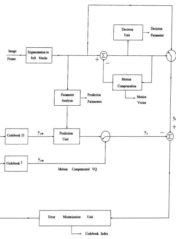
CODER STRUCTURE

The block diagram of the coder is shown in Fig2.1. At the coder the original image is first divided into

8

x

8

blocks. Motion compensation is used in order to exploit the redundancy along the temporal direction. The motion vectors are found using the block-matching method [35]. For each

8

x

8

block a motion vector, whose two integer components range from —7 to +7, is determined.

There are a total of four different coding strategies used in this coding system. Each block is coded independently of other blocks in the frame. A decision about one of the four coding methods is taken by looking at the value of the Displaced Frame Difference (DFD) for the block. After the motion compensation is applied, DFD of the (A:,/)’th block with motion vector u =

(ux,Uy), DFDkt{ux,u,j), is determined by using

2

.

1

,

8(A:+l)-18(i+l)-l

DFDkiiu^.Uy) = Y \ X r , { i , j ) - X n - i { i - u ^ , j - U y ) \ (2.1)

izzSk j=8l

where A '(.,.) represents the image intensity and the subscript n shows the frame number of the image.

Three experimentally chosen thresholds (T^, T\ and Tj) are used to deter­ mine the type of the coding scheme for the

8

x

8

image blocks.

0. No coding :

{DFDki{ux,Uy) < Ti and j DFDki{u^,Uy) - DFDki(0,0) |< Tm)

8

This case occurs when there is almost perfect matching in the motion compensation, and there is not much reconstruction error if (

0

,

0

) motion vector is sent in stead of the real motion vector. Usually this type of image blocks are encountered in the background of the images.

1

. Coding using only the motion information :

(DFDki{ux,Uy) < Ti and |DFDkiiux,Uy) - DFDki{0,0) |> Tm)

This case also occurs when there is almost perfect matching in the motion compensation and there is a significant advantage in sending the real motion vector instead of the (0,0) motion vector. Usually this type of blocks are encountered on the hair of the speaker.

2

. Coding using motion information in combination with VQ :

(Ti < DFDki{u^,Uy) < T2)

In this case the DFD is larger. Motion compensated error signal is vector quantized. This motion information provides the temporal prediction of the block. The motion data as well as the temporal prediction error are required at the receiver to reconstruct the block.

3. Predictive coding with VQ : {T2 < DFDki{ux,Uy))

In this case the DFD is quite large, i.e., these parts of the image have the highest temporal activity. Since temporal prediction proves to be useless, motion information is not used at all. Image intensity signal itself is coded using spatial prediction and VQ. Prediction error for each block is vector quantized.

At every block of the image, first the decision parameter about the coding strategy used for that block is sent by the coder to the decoder.

If the current block is of type 0, nothing else is transmitted other than the decision parameter.

If the current block is of type

1

, only the motion vector is sent by the coder to the decoder, in combination with the decision parameter.

If the current block is of type 2, motion compensated error block is vector quantized. Vector quantizer codebook (Codebook I) is searched for the code­ word that is most similar to the original motion compensated image block. Similarity criterion used by the vector quantizer is given as follows.

Figure

2

.

1

: Coder structure.

¿ = 0 j= 0

(2.2)

where and shows the codeword read from Codebook I and the orig­ inal motion compensated image block, respectively. Index of the codeword that minimizes the difference measure in

2

.

2

, and the motion vector are the parameters that are transmitted with the decision parameter.

If the current block is of type 3, then the prediction parameters are cal­ culated using the image data in the block. These parameters are fed into the predictor. The predictor, using the prediction parameters, constructs the prediction filter. Afterwards, the best-matching codeword is searched from the prediction based vector quantizer codebook (Codebook II) which minimizes the difference between the original image block, and the reconstructed image block, Up. The reconstructed block, v^, is obtained using.

E,(>, j ) = Hpihj) + (2.3)

where represents the predicted block, and represents the codeword that plays the role of an error signal between the predicted and the original pixel values. The error criterion between the original and the reconstructed image blocks is chosen to be the sum of the absolute differences at each pixel site in the block, i.e..

1 = 0 j= 0

(2.4)

For type 3 blocks, parameters transmitted are the prediction parameters, code­ book index of the best matching codeword of Codebook II and the decision parameter.

Chapter 3

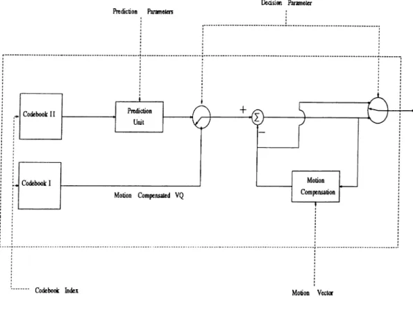
DECODER STRUCTURE

The decoder is shown in FigS.l. Inputs to the decoder are the decision pa­ rameter which determines the coding method used for the current block of the image, codebook index which determines the codeword that will be read from the codebook, prediction parameters which are used in the construction of the spatial prediction filter and the motion vector that is used in the temporal prediction.

If the current block is of type 0, previously decoded image frame is used to reconstruct the block. Let the current block be the (A;,/)’th block of the n ’th image frame. The reconstructed image block is obtained by just copying the block with the same position in the previously decoded image to the current image frame as shown in .3.1,

Xn(Sk +

8

/ + j ) — Xn-i{Sk + I, SI + j ) 0 < i J < S (3.1) where Xn(i~j) and Xn- \{hj ) represents the reconstructed image intensity sig­ nals at the (i,j) pixel position for the n ’th and (n — l ) ’st frames, respectively. If the current block is of type

1

, only the motion vector and the buffered previously decoded image frame is used to reconstruct the block at the decoder. Let the current block be the ( ¿ , / ) ’th block of the n ’th image frame, and u = (ux, Uy) show the motion vector for that block. Then the reconstructed image block is obtained using 3.2,

Decision Parameter

Figure 3.1: Decoder structure.

Xfi[8k + i·)

8

/ 4"

7

) — Xn—i i — Ux, 81 j — Uy) 0 ^

7

■<8 (3.2)

If the current block is of type 2, codebook index is used to get the vector quantizer codeword from Codebook I. Using the motion vector accompanied by the vector quantizer codeword, block is synthesized at the decoder side. With the same notation as above, reconstructed image signal for type 2 blocks is obtained using 3.3,

Xn(^k-\-i,8l-\-j)

— .^n-i(8A:+i—Uj;,8/+ji—ity)+U(,u,(i,_;)

0 < i,j < 8 (3.3)

It is not difficult to notice that the coding method for blocks of type

1

is the same for that of type

2

except the difference that in type

1

, v^yj is always taken to be 0. Because for the blocks of type 1 motion compensated error signal is not coded.

If the block is of type 3, then the prediction filter is reconstructed by the

knowledge of the prediction parameters. Suitable codeword is read from Code­ book II, using the codebook index received. Via 3.4 and 3.5 reconstructed image block is obtained by the decoder.

Vrihi) = V.p{hj) + Vcwihj) 0 < i,j < 8 (3.4)

Xn{^k + ¿ ,₈/ + j ) = v^{i,j) ₀ < i , j < ₈ (3.5)

Chapter 4

THE PREDICTION UNIT

The simplest model of an image is a set of discrete random variables (the pixel intensity values) in a two dimensional array, i.e., with each pixel statistically independent from any other pixel. If this model were correct, PCM coding would be perfectly adequate to encode the image concisely. Because PCM does not exploit any redundancy in the form of correlations of the pixel intensities, instead it considers every pixel to be totally independent of others. However this is not the case. A more realistic model is that of a 2D array of pixel intensities with high dependencies (or correlations) between closely neighboring pixels. By optimal selection of the prediction filter we can remove a great deal of the correlation between pixels, thus leaving a more statistically independent residual image, which is more suitable for VQ coding. Dependency of VQ on the training sequence diminishes for low correlated signal sources. This provides the compression power of multi-source coding in video applications with global- like codebooks [36]. Also by decreasing the dependency of the VQ codebook on the training sequence, the coding scheme becomes more robust to changes in the input signal. After spatial prediction, unpredictable part of the image signal is left to be vector quantized. Therefore, the VQ codebook contains several edge structures that are mostly encountered in head and shoulders type of images. It is easy to code the predictable part of the signal by just sending the prediction parameters for the block. But if the predictable part was also vector quantized this would give rise to larger overall reconstruction error.

Two different prediction methods are used in the video codec, and their

effects on the codec performance are compared. Prediction methods examined are :

(i) Linear prediction, and

(ii) Gibbs random field(GRF) model based non-linear prediction.

Both of the prediction methods are causal in the sense that, in the recon­ struction stage previously decoded image pixels are used in predicting other pixels. Only spatial prediction is used, i.e., for the blocks that are coded using predictive VQ, no motion compensation (temporal prediction) is used. Also prediction is adaptive, meaning that the prediction parameters are updated in each image block.

In the sections that follow, linear and GRF model based non-linear predic­ tion methods and the calculation of the prediction parameters will be investi­ gated in detail.

4.1

Linear Prediction

Individual pixel intensities can be thought of as a linear combination of other neighboring pixel intensities, plus a more random (or uncorrelated) residual signal. Such dependencies can be expressed as in 4.1,

^ { h j ) = - k j - l) + e { i j ) (4.1)

k I

where X { i , j ) is the image intensity at pixel location (i,j), is the residual signal, and aki are the so called linear prediction coefficients, and (k,l) run over some definable region of support. The above equation in fact describes an infinite impulse response (HR) filter, and the process is known as linear predictive (LP) filtering [37] [38] [39] [40] [41].

In our case we take the LP support to be consisting of three neighboring pixels. For the formulation that follows pixel configuration given in Fig4.1 is taken to be the basis.

Let the pixel values X{ i — l , i ) , X { i i j — 1) and X{ i — l , j —

1

) be given,

X{ i i j ) is desired to be predicted linearly using the pixel values that are given.

X ( i - l J - l ) X ( i - i J )

X ( i J - i ) X ( i J )

Figure 4.1: Pixel configuration for linear prediction.

Therefore prediction for X { i , j ) , X{ i , j ) , can be expressed as a linear superpo­ sition of X{ i — l , j ) , X { i , j — 1) and X( i — l , j —

1

) as in

4

.

2

,

X { i , j ) = a X ( i J - 1) -f- bX{i - I J - 1) + cX{i - l , j ) (4.2) Therefore the residual signal can be expressed as,

6{ i J) = X i i J ) - X ( i J )

= X { i J ) - a X { i J - 1) - bX{i - l , i - 1) - cX{i - I J ) (4.3) Total mean square error (MSE) for the block will be,

E = = J ^ ( X ( i , j ) - a X ( i J - l ) - i X ( i - l J - l ) - c X ( i - l , j ) y (4.4)

Prediction parameters a, b, and c are desired to be chosen such that the total prediction error E is minimized. Therefore we take the partial derivatives of

E with respect to a, b and c, and equate them to zero.

dE ^

d a ~ ^ db =

0

dE ^

These three linear equations in three unknowns give rise to a 3x3 matrix equa­ tion stated in 4.5, r (

0

,

0

) r ( l ,

0

) r ( l , l ) r ( l ,

0

) r (

0

,

0

) r (

0

, l ) a r (

0

,

1

) b = r ( l , l ) c r ( l ,

0

) _ (4.5)

where r ( . , .) is the autocorrelation function which is defined as in 4.6,

r(m,

n) =

(4.6)

where is the image intensity at pixel position (i, j) and summation is over the block of the image.

4.2

GRF model based non-linear prediction

A causal Gibbs random field (GRF) based statistical model is assumed for the image intensity signal. A different notation will be used to investigate the non-linear prediction method proposed in this study. In this section following notation will be used :

L : 2D array {lattice) of points,

77

,j : set of points that are in the neighborhood of the point (¿,

7

),

Xij : random variable at point (i,j),

X { i , j ) : realization of the random variable at (i,j), ¡3 : any subset of L,

x(/?) : numerical realization of subset of pixels constituting /

0

,

P : probability assignment function.

Image intensity function is modeled as a

2

D array of random variables, over a finite N\xN2 rectangular lattice of points (pixels) defined as

L = { { h i ) :

0

< ¿ < A^i,

0

< i < A

^2

}

The description of a Gibbs random field is based on the definition of a neigh­ borhood structure on L. [42] [43]

A collection of subsets of L given by

{ Vij ·’ Vij ^ ^ }

is a neighborhood system on L if and only if the neighborhood, t]ij, of a point

{ifj) is such that :

(*>i) t Vij and

Figure 4.2: First order causal neighborhood structure used in GRF model based non-linear prediction

(i) (ii) (iii)

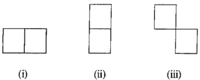
Figure 4.3: Cliques associated with the selected the neighborhood system.

ik,l)^Vi3 {iJ)^Vkh y { i , j ) e L

In this study, the shape of the neighborhood of an inner point of L is assumed to be independent of the position of the point (pixel) in the image region L. A causal first order neighborhood shape, which is shown in Fig4.2, is entertained in the random field model.

The “cliques” associated with a lattice-neighborhood pair {L,r]) is defined as follows.

A clique of the pair denoted by c, is a subset of L such that,

(i) c consists of a single pixel, or

(ii) for (¿ ,j)

7

^ (A:,/), ( * , i ) G c and {k,l) e c ik,l)eTjij

The types of cliques associated with the neighborhood shape given in Fig4.2 are shown in Fig4.3. As it is noted, each type of clique consists of two pixels in the horizontal, vertical and diagonal directions.

A Gibbs random field is a probability assignment on the elements of the set of all numerical realizations x, subject to the following condition (Markovian property) :

P { X ( i , j )

I x (i\{(i.j)))) =

P (X (i,J )

I

x M ) ,

V(i,j)

€

L

Some preliminary definitions are given, but in order for a random field model to be totally established, joint distribution probability function must be defined.

Let

7

/ be a neighborhood system over the finite lattice L. A random field

X = { Xij } defined on L has a Gibbs distribution (GD) or equivalently is a Gibbs random field with respect to rj if and only if its joint distribution is of the form,

P [ X = x) =

where X is the random field, x is the realization of the random field (i.e., a specific image) and U{x) is the so called energy of the image. The partition function Z is simply a normalizing constant. Energy function can be expressed as.

u ( x )= k (x) alt c

where Vc(x) is the potential associated with clique c. The only condition on the otherwise totally arbitrary clique potential Vc{x) is that it depends only on the pixel values in the clique c.

A maximum likelihood (ML) prediction is assumed. Let the pixel values at positions —1), (¿—l, y —

1

) and (i — l , j ) be given as —

1

), X { i —l , j — l)

and X ( i — l , i ) , respectively. GRF model based non-linear prediction tries to find X ( i , j ) such that the following probability is maximized.

P { X , , \ X { h , i y , h j t i , l ^ j ) (4.7) Since Markovian property is assumed to hold, probability expression in 4.7 is equivalent to the one in 4.8,

P{Xi, I X( i - i j f X { i - I ,i - l ) , X ( i , i - 1)) (4.8)

Therefore, the prediction process is reduced to the maximization of the proba­ bility of the numerical realization of a pixel in the image, given the pixel values of its neighbors. Since the probability of an image is given in the following form,

P { X ^ x ) = Zl

maximization of the probability is the same as the minimization of the energy function U{x). Hence, the prediction is nothing but an optin. ,tion process on the energy function.

In this study, energy function U{x) is chosen as shown in 4.9,

U { X { i , j \ X { i - - l)^X{i - l , i - 1)) = n . D k . D , , D , ) (4.9) where, ' - 1 , i f \ X { i J ) - X { i J - i ) \ < T Dk = D , = -(-

1

, otherwise - 1 , \ i \ X { i , j ) - X { i - \ , j ) \ < T -|-

1

, otherwise

-1,

\ i \ X ( i , ] ) - X ( i - U ] - \ ) \ < T +

1

, otherwise

where T is a pre-selected threshold.

4.2.1

Estimation of the non-linear prediction parame­

ters

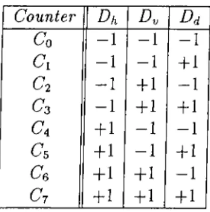
Dhi Dy and Dd can take two different values, namely —1 and -f-l. Therefore, there are a total of

8

different configurations for the triple {Dh, Dy, Dd), as shown in Table4.1.

Eight counters are assigned to the values of the triple {Dh, Dd) :

6

^

0

, ••mC'?. In each block of the image

8

counters are initialized to zero. Then all of the pixels in the block are visited. Depending on the value of the triple

{Dh,Dy, Dd) corresponding counter is increased by one, while the others are

Counter Dh By Bd Co - 1 - 1 - 1 C: - 1 - 1 +1 C2 - 1 + 1 - 1 Co - 1 +1 + 1 C4 +1 - 1 - 1 Cs + 1 - 1 +1 Ce +1 +1 - 1 C7 _{+1 +1 +1}

Table 4.1: Counter assignment to the triple {Dh·, D^, Dj).

not eíFectecl. For example, if we encounter the following case in the block,

I

X( , , j ) - X(z - l , j )

|<

T \ x { i , i ) - x ( i , i - i ) \ < T \ x { t , } ) - x { i - i , j - i ) \ < T

i.e., {Dhi Dy, Dd) = (+1, +1, +1), then the counter Cj is increased by one while the other counters are kept constant. It is not difficult to notice that,

Yii=o — number of pixels visited in the block

After all of the pixel sites in the block are visited, the indices of three coun­ ters with highest values are saved and transmitted as the prediction parameters for the block. For example, after all of the pixels in a block are visited and following counter values are calculated,

Co = 2, C\ = 0 , C2 = 0, Co = 0,

C4 = l,

C,5 = 6, C(j = 10, ^7 = 30

then the prediction parameters will be (pi,P2,P3) = (7,6,5). As it is noted, there are a total of 8x7x6 = 336 different combinations for the prediction pa­ rameters. Without any further coding, 9 bits are required to code the prediction parameters of a block.

4.2.2

Non-linear prediction process

Given the prediction parameters ipi,P2,P3) and the pixel values X{ i — 1,^), _ I) and X { i J - 1), the prediction process has the following steps :

1. Take the first prediction parameter p\ (i.e., the index of the counter with the highest value)

2. Try to find an X { i , j ) such that {Dh, Dy, Dd) triple value corresponding to Cp, is satisfied.

(i.e., if Pi = 7 for example, try to find X { i , j ) such that :

\ X ( i , ] ) - X { t J - l ) \ < T

\ X ( i , j ) - X { i - l , j - i ) \ < T )

3. a. If only one X { i , j ) is found, take it to be the prediction for the point

i h j )

b. If more than one value is found, select one of them depending on the following rule :

min { +

D , \ X ( , J ) - X ( i - \ , j ) \ +

£ > i | , V ( i , y ) - A ' ( i - I , ; - l ) | )

c. If no value is found satisfying Cp,, take the second prediction pa­ rameter, P'

2

, and try to find an X{i, j ) such that {Dh, Dy, Dd) triple value corresponding to Cpj is satisfied, (i.e., do the steps 1 thru 3 above with p2 instead of pi) If the prediction proves to be unsuccess­ ful with p

2

also, take pa as the prediction parameter. If a prediction for X { i , j ) is not found using all of the prediction parameters (which is rarely the case), prediction for X { i , j ) is obtained by taking the three point median of X{ i — 1, j ) , X{ i — l , i — 1), and X { i , j — 1).

Chapter 5

VECTO R QUANTIZER

DESIGN ALGORITHM

In the vector quantizer design, the Linde-Buzo-Gray (LBG) algorithm is used. A brief explanation about LBG algorithm is given in this section, but for more detailed information and/or its applications to different problems see [44] [45]

(461

[

47

|

1

'I

8

|.

The general LBG algorithm iteratively improves a given codebook for a given source probability density function (PDF). In practice however, the source PDF is not known a priori, therefore the algorithm must use instead a sequence of training data which is assumed to be similar to the image sources that will be coded later. In this way estimate of the PDF is formed from a pre-known training set. In our case we used several “head and shoulders” type of images in training of the vector quantizer, since the codec will be used for the video-phone applications.

Starting from the given codebook, each vector in the training set is clustered around its closest match in terms of MSE, in the codebook to form a population of training vectors for each codeword. A new codebook is then formed by taking the centroid of each cluster. This procedure is then iteratively repeated, leading to a monotonically decreasing total training set error for the codebook being designed.

There are several ways of choosing the initial codebook :

(i) as a series of random vectors,

(ii) as a series of vectors equally distributed in Euclidean space, as in uniform scalar quantization,

(iii) by using the centroid of the whole training set as an initial codeword, and then splitting algorithm to increase the number of codewords to 2, then to 4, then to 8, etc.

Since the third approach is implemented in the vector quantizer design algo­ rithm used in this thesis, codeword splitting algorithm will be explained in a little bit detail in the rest of this section.

In the codebook splitting algorithm, codebook is started off with a code­ word, say X, which is taken to be the centroid of the entire training set. This vector is then split into two vectors by a small perturbation vector, e. Thus there are now two vectors, (x 4 - e) and (x — e). The LEG algorithm is then applied to this new codebook to form a better two-word codebook. Each code­ word is then split into two words, and LEG algorithm is used again. At each step the number of codewords is doubled, and the LEG algorithm is applied to optimize the new codebook.

5.1

Preparation of the training sequence

In the codec structure there are two different codebooks. Codebook I and Code­ book II, which are used in the coding of type 2 and type 3 blocks, respectively. Therefore, two training sequences with different characteristics are generated to be used in the design of the codebooks. Eoth of the training sequences are made up of blocks of error-like signals.

First training sequence contains motion compensated block differences. Let

Xn{ i , j ) and Xn- i { i , j ) be the image intensity values at spatial coordinate on the two consecutive image frames which are used in the training process. And let u = (lij,, Uy) be the motion vector associated with (k, / ) ’th block of the n ’th image frame. Then the training sequence element, Vi{i,j) obtained from the (A:,/)’th block of the n ’ th frame is constructed by using 5.1.

lltihj) — Xn{^k-\-i,8l-\-j) — Xn-ii^k-\-i — Ux,8l-\-j — Uy) 0 < i , j < 8 (5.1)

Second training sequence contains the spatial prediction error signals. Let

2lo{hj) be the original image block, and Up(z, j ) be the prediction for it, then the training sequence element,^(z, j ) , is obtained using 5.2,

0 < i , j < 8 (5.2)

If prediction is not used in the codec then in generating the training se­ quences Vp in 5.2, is taken to be 0 and again two different codebooks for vector quantization of type 2 and 3 blocks are generated.

Chapter 6

SECOND LEVEL CODING

At each block of the image some parameters are extracted from the image by the coder and then those parameters are transmitted to the decoder. Decoder, using those parameters synthesizes the image at the receiver. Extraction of the parameters is called the first level coding. In the first level coding, greatest part of the compression is achieved. But when the parameters themselves are coded further (i.e., not transmitted in their own raw format), compression ratio is increased by a non-negligible amount. This process, coding of the parameters of the first level coding further, is called the second level coding.

A block of the image can be of four different types : 0, 1, 2, or 3. Parameters that must be transmitted for each type of block are known by the coder and the decoder. They are listed below :

0. decision parameter. 1. decision parameter, motion vector. 2. decision parameter, motion vector, codebook index. 3. decision parameter, codebook index, prediction parameters.

27

Event Approximate percentage Assigned codeword Number of bits type 0 65 0 1 type 1 20 1 0 2 type 2 10 1 1 0 3 type 3 5 1 1 1 3

Table 6.1: HufFman code table for decision parameter with no grouping.

Prediction parameters are vector quantized. The number of levels in the vector quantizer for the prediction parameters and the sizes of Codebook I and Codebook II are known a priori by the coder and the decoder. No further coding scheme is used for the codebook index and prediction parameters. The codebook and the prediction parameters’ vector quantizer index are transmit­ ted directly. .Second level coding is applied to the motion vector and decision parameter only. In the following sections methods used to code the decision parameter and the motion vector will be stated in detail.

6.1

Decision parameter

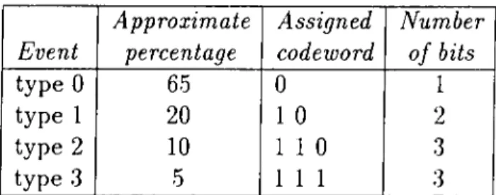
Decision parameter can take four different values (0,1,2,3) showing the type of the coding scheme for the current block. Therefore, if decision parameter is transmitted in its raw format, 2 bits per block is required. Instead, Huff­ man coding [49] is adapted for the decision parameter. Huffman coding is an effective way of reducing the number of bits used to represent events with non-uniform probabilities. Events with larger probability are coded with fewer number of bits, on the other hand less probable events are coded with more bits. Two different Huffman coding schemes can be applied to the decision parameter.

(i) With no grouping of events : It is experimentally observed that, on the average 65 percent of blocks is of type 0, 20 percent of blocks is of type 1, 10 percent of blocks is of type 2, and 5 percent of the blocks is of type 3. .Since the probabilities are not the same for the events Huffman coding will give rise to a reduction of the number of bits per decision l)arameter. Statistical results, codeword assigned to each value of decision

Event Approximate percentage Assigned codeword Number of bits type 0 (length 1) 14 0 1 1 3 type 0 (length 2) 8 0 0 11 4 type 0 (length 3) 5 1 1 1 1 4 type 0 (length 4) 3 1 1 1 0 0 5 type 0 (length 5j 5 0 0 0 1 1 5 type 0 (length 10) 2 0 0 0 0 1 0 6 type 0 (length 25) 2 0 0 0 0 1 1 6 type 0 (length 50) 0.4 0 0 0 0 0 0 0 0 8 type 0 (length 100) 0.6 0 0 0 0 0 0 0 1 8 type 1 (length 1) 18 1 0 2 type 1 (length 2) 7 0 1 0 0 4 type 1 (length 3) 4 0 0 1 0 0 5 type 1 (length 4) 2 0 0 0 0 0 1 6 type 1 (length 5) 3 1 1 1 0 1 5 type 2 (length 1) 10 1 1 0 3 type 2 (length 2) 4 0 0 1 0 1 5 type 2 (length 3) 2 0 0 0 1 0 0 6 type 2 (length 4) 1 0 0 0 0 0 0 1 7 type 2 (length 5) 2 0 0 0 1 0 1 6 type 3 (length 1) 7 0 1 0 1 4

Table 6.2: Huffman co<le table for decision parameter with grouping.

parameter and the number of bits used to represent each event are shown in Tabled. 1. With this method, average number of bits for coding the decision parameter is achieved as 1.5 bits per block.

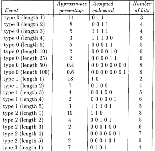
(ii) With grouping of events : In this case the events are grouped, because of the experimental observation that type 0, type 1 and type 2 blocks are distributed on the image as bundles. Type 0 blocks which are usually encountered on the background of the image ha,ve larger groups (some­ times up to a few hundreds of consecutive type 0 blocks), compared to type I and type 2 blocks (maximum length of the groups for type 1 and type 2 blocks is around 10). On the other hand type 3 blocks are not en­ countered as bundles on the image. Therefore, several groping structures are selected for types 0, 1, and 2, and no grouping is assumed for type 3. Selection of events, statistics associated with, codewords assigned to and number of bits used for each event are presented in Table6.2. With this method average number of bits for coding of the decision parameter is reduced to 1.0 bit per block.

6.2

Motion vector

Motion vector is coded differentially. Let the current motion vector be = (ucj,Ucy) fhs previous motion vector be = (up^, Wpj,)· Difference motion vector,

= (l\U a;, Z\Uy) = ( ^ C i ^ P x i ^ C y ^ P j / )

is coded. Since,

we have,

—7 < iix, Uy < 7

— 14 < Au^;, Auy < 14

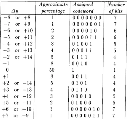
Normally, 5 bits is required to represent Aux (or Auy) therefore 5x2=10 bits to represent the full motion vector. In order to decrease the number of bits spent for motion vector representation, Huffman coding is implemented. Events are defined to be the components of the difference motion vector. First, the statistics about the events are obtained by using some typical image se­ quences, and then Huffman code table is generated.

Au Approximate percentage Assigned codeword Number of bits - 8 or -1-8 1 0 0 0 0 0 0 0 7 - 7 or 4-9 1 0 0 0 0 0 0 1 7 - 6 or 4-10 2 _{0 0 0 0 1 0 6} - 5 or 4-11 2 0 0 0 0 1 1 6 - 4 or 4-12 3 0 1 0 0 1 5 - 3 or -bl3 4 0 0 0 1 1 5 - 2 or 4-14 5 0 1 1 1 4 - 1 8 0 0 10 4 0 50 1 1 +1 8 0 0 11 4 +2 or —14 5 0 1 0 1 4 +3 or —13 4 0 1 1 0 4 +4 or —12 3 0 0 0 1 0 5 +5 or —11 2 0 1 0 0 0 5 +6 or —10 1 0 0 0 0 0 1 0 7 +7 or —9 1 0 0 0 0 0 1 1 7

Table 6.3: Huffman code table for motion vector.

At each block Aur and are coded independently (and consecutively). The same Huffman code table is used for both Au^ and Auy. Initially, at the beginning of each frame,

Up^ = 0 and Up^ = 0 is assumed.

Via the Huffman coding, average number of bits used for one component of the motion vector is reduced from 5 bits to 2.8 bits. Therefore, 2.8x2=5.6 bits is required to code a motion vector fully.

In Table6.3 statistics, assigned codewords and the number of bits for rep­ resentation of motion vector is presented.

Chapter 7

SIMULATION RESULTS

Simulations are conducted using “Miss America” , “Claire” and “Trevor” im­ age sequences. All of these sequences are made up of the so called head and shoulders type of color images. All of the images are originally in the Com­ mon Intermediate Format (CIF). CIF has Y, U, V representation for color images. Y component (luminance) has dimensions 288x352, U and V compo­ nents (chrominance differences) have the dimensions 144x176, and each pixel is represented by 8 bits. First frames of these three sequences are shown in FigT.l, Fig7.2 and Fig7.3.

In the simulations Y, U and V components of the image signal are coded sep­ arately in order to have the modularity. This enables the receiver to choose only the luminance part of the coded signal and decode it to watch a black/white scene. During the coding process each image frame is divided into blocks. Size of each block is 8x8 for Y component and 4x4 for U and V components. The selection of block size for Y component is due to the frequent use of 8x8 block size in the literature. Also, since VQ coding algorithms are used, large block sizes decrease the effectiveness of VQ. On the other hand small block sizes are not appropriate to the image coding application studied in this thesis, since us­ ing small blocks decreases the compression ratio. In order to have a one to one correspondence of the blocks of Y, U, and V components of the image signal, block size is determined to be 4x4 for the color components. By this selection the number of blocks in the Y, U and V components are the same, and they can be matched in a one to one manner. Three blocks (8x8 luminance block with two 4x4 chrominance difference blocks) constitute a color (image) block.

Figure 7.1: First frame of the “ Claire” sequence.

Figure 7.2: First frame of the “ Miss America” sequence.

Figure 7.3: First frame of the “Trevor” sequence.

Without any coding a color block is represented by (8x8 + 4x4 + 4x4)x8 = 768 bits.

Prediction parameters are vector quantized to 256 levels (8 bits). Motion vector and decision parameter are Huffman coded to 2x2.8=5.6 bits and 1.0 bits per block, respectively. VQ codebooks used in vector quantizing the mo­ tion compensated error blocks are separately designed for the Y, U, and V components and they are the same for the codecs making use of linear and GRF model based non-linear prediction. Predictive VQ codebooks, on the other hand, are also separately designed for Y, U, and V components, but they are not the same for linear and non-linear prediction based codecs. In design­ ing the vector quantizer codebooks LEG algorithm is used whose details are explained in Chapter 5. The reason for the selection of LEG algorithm is the fact that it is the most widely used and well performing clustering algorithm in the literature. Also, several studies in the literature concluded that the LEG algorithm is suitable for use in the video compression algorithms.

For video-phone application the images are expected to be standardized in the Quarter Common Intermediate Format (QCIF). QCIF has Y, U, V representation for color images. Y component has dimensions 144x176, U and V components have dimensions 72x88 and each pixel is represented by 8 bits. Also, expected standardization for the number of frames falling on to the screen per second (frame rate) is in between 5.00 Hz and 8.33 Hz. Throughout