DEMAND AND SUPPLY OF REAL ESTATE MARKET IN TURKEY: A COINTEGRATION ANALYSIS A Master’s Thesis by ZEYNEP BURCU BULUT Department of Bilkent University Ankara January 2009
To My Husband and My Family
DEMAND AND SUPPLY OF REAL ESTATE MARKET IN TURKEY: A COINTEGRATION ANALYSIS The Institute of Economics and Social Sciences of Bilkent University by ZEYNEP BURCU BULUT In Partial Fulfilment of the Requirements for the Degree of MASTER OF ARTS in THE DEPARTMENT OF ECONOMICS BİLKENT UNIVERSITY ANKARA January 1999
I certify that I have read this thesis and have found that it is fully adequate, in scope and in quality, as a thesis for the degree of Master of Arts in Economics. ‐‐‐‐‐‐‐‐‐‐‐‐‐‐‐‐‐‐‐‐‐‐‐‐‐‐‐‐‐‐‐‐‐ Assoc. Prof. Çağla Ökten Supervisor
I certify that I have read this thesis and have found that it is fully adequate, in scope and in quality, as a thesis for the degree of Master of Arts in Economics. ‐‐‐‐‐‐‐‐‐‐‐‐‐‐‐‐‐‐‐‐‐‐‐‐‐‐‐‐‐‐‐‐‐ Asst. Prof. Ümit Özlale Examining Committee Member
I certify that I have read this thesis and have found that it is fully adequate, in scope and in quality, as a thesis for the degree of Master of Arts in Economics. ‐‐‐‐‐‐‐‐‐‐‐‐‐‐‐‐‐‐‐‐‐‐‐‐‐‐‐‐‐‐‐‐‐ Assoc. Prof. Zeynep Önder Examining Committee Member Approval of the Institute of Economics and Social Sciences ‐‐‐‐‐‐‐‐‐‐‐‐‐‐‐‐‐‐‐‐‐‐‐‐‐‐‐‐‐‐‐‐‐ Prof. Erdal Erel Director
ABSTRACT DEMAND AND SUPPLY OF REAL ESTATE MARKET IN TURKEY: A COINTEGRATION ANALYSIS Bulut, Zeynep Burcu M.A., Department of Economics Supervisor: Assoc. Prof. Çağla Ökten January 2009 Since in a country the housing market is a leading indicator for the whole economy, the determinants, that are affecting aggregate housing supply and demand, are widely searched. In this study, we try to find the variables which are affecting the demand and supply of real estate market in Turkey between the years 1970 to 2007. We can not specialize on the housing market and rather study the real estate market in the aggregate‐‐‐number of dwellings is our quantity measure‐‐‐due to data limitations. We chose Topel and Rosen’s (1988) demand and supply models that are basically based on different short‐ and long‐run elasticity. As demand side independent variables, interest rate, value variable, income and population are chosen and as supply side independent variables, value, interest rate and costs are chosen.
Value is used as a proxy since the market price data does not exist in Turkey. Value is a kind of cost that is taken from the builder without interested in what the materials are and how much the labor costs to the builder. Also, the annual data is used because of the data limitations. Due to the fact that all these variables are I(1), Johansen Cointegration and VECM are preferred. According to the empirical findings, the signs of all the variables are as expected and are significant in the long‐run. However, in the short‐run, only interest rate and cost variables are significant in 90% confidence level. Furthermore, the price elasticity of supply is 1.5 in the long‐run while it is 0.13 in the short‐run. This shows us that the adjustment costs for a change in Turkey is significantly high. Moreover, the long‐run price elasticity of demand is ‐4.97.
Keywords: Housing supply, housing demand, cointegration, vector error correction
ÖZET TÜRKİYE’DE GAYRİMENKUL PİYASASI ARZ VE TALEP DENGESİ: EŞBÜTÜNLEŞME ANALİZİ Bulut, Zeynep Burcu Yüksek Lisans, İktisat Bölümü Tez Yöneticisi: Doç Dr. Çağla Ökten Ocak 2009
Bir ülkede konut piyasası, genel ekonomi açısından gösterge niteliği taşıdığından dolayı, konut piyasası toplam arz ve talep bileşenleri yaygın bir şekilde araştırılmıştır. Bu çalışmada, 1970 ve 2007 yılları arasında Türkiye gayrimenkul piyasası toplam arz ve talebi oluşturan değişkenler bulunmaya çalışılmıştır. Veri eksikliğinden dolayı, özel olarak konut piyasası incelenememişti. Birbirinden farklı uzun ve kısa dönem fiyat elastikiyetleri esasına dayalı olan Topel ve Rosen (1988) konut arz ve talep modeli tercih edilmiştir. Konut piyasası yazınında sıkça kullanılan talep/arz değişkenleri esas alınarak, bu çalışmada telep değişkenleri olarak, nüfus, faiz oranı, gelir ve değer değişkenleri; arz denge değişkenleri olarak, değer, faiz oranı ve maliyet endeksi değişkenleri kullanılmıştır. Değer datası, Türkiye’de evlerin piyasa fiyatları bulunmadığından dolayı, fiyat değişkenine vekil olarak
kullanılmıştır. Ayrıca, bina sayısı verisi yıllık olarak toplanmasından dolayı, bu çalışma yıllık veri ile gerçekleştirilmiştir. Bütün değişkenlerin birinci farkları durağan olduğundan dolayı, Johansen Eşbütünleme ve Hata Düzeltme Modeli tercih edilmiştir. Bu çalışmanın ampirik sonuçlarına gore, uzun dönemde söz konusu arz/talep değişkenleri anlamlı çıkmıştır ve beklenen işaretler görülmüştür. Buna karşın, kısa dönemde faiz oranları ve maliyet değişkenleri dışında bütün değişkenler %90 güven seviyesinde anlamsız çıkmıştır. Ayrıca, uzun dönem arz fiyat esnekliği 1.50 olarak çıkarken, kısa dönem arz fiyat esnekliği 0.13 olarak çıkmıştır. Söz konusu esneklik sayıları bize, konut piyasasında olan bir değişikliğin kısa dönemde gerçekleşme maliyetinin çok yüksek olduğunu göstermektedir. Ayrıca, uzun dönem talep fiyat esnekliği ‐4.97 olarak çıkmıştır.
Anahtar kelimeler: Konut Talebi, konut arzı, Eşbütünleşme, Vektör Hata Düzeltme
ACKNOWLEDGEMENTS
I feel most fortunate to have been guided and supervised by my advisor, Assoc. Prof. Çağla Ökten and would like to express my deepest gratitude to her for her valuable recommendations, patience and guidance which helped me finish this study. I would also like to thank Asst. Prof. Ümit Özlale and Assoc. Prof. Zeynep Önder for their valuable critique and comments on my thesis. Without their suggestions, I would not have been able to improve the academic quality of my thesis.
My thanks should go also to my husband, my parents and my brother for their continuous support, encouragement and motivation in the really hard times I lived through.
I am grateful to my friends at Bilkent University for their useful comments, moral support and close friendship. Without their help, I would never be able to complete this study.
I also want to thank to Vakıfbank for the support during my graduate study. Especially I owe thanks to my colleagues and my manager, Cem Eroğlu, in Economic Research Department at Vakıfbank for their great understanding and enforcing me to finish my graduate study.
TABLE OF CONTENTS
ABSTRACT………...………… iii ÖZET……… v ACKNOWLEDGEMENTS………...… vii TABLE OF CONTENTS………. viii LIST OF TABLES……… x LIST OF FIGURES……… xii CHAPTER 1: INTRODUCTION………...………... 1 CHAPTER 2: LITERATURE REVIEW ... 5 CHAPTER 3: HOUSING INVESTMENT THEORY ... 10 3.1 Housing Supply ……….……….… 12 3.2 Housing Demand ……… 19 3.3 Implications of Theory ……… 25 CHAPTER 4: HOUSING MARKET IN TURKEY ………….. 29CHAPTER 5: ECONOMETRIC METHODOLOGY AND DATA ... 35 5.1 Methodology ……..………... 35 5.1.1 Phillips Perron Unit Root Test….………. 36 5.1.2 Johansen Cointegration Test ………... 38 5.1.3 Vector Error Correction Model ……… 42 5.2 Data ……….………... 44 5.3 Econometric Model ……….. 48 CHAPTER 6: ESTIMATION RESULTS ………... 52 6.1 Empirical Results of Housing Supply and Demand ..… 53 6.1.1 Level Data Analysis ………. 54 6.1.2 Logarithmic Form Analysis ……… 63 6.2 Limitations of Results ……….... 67 CHAPTER 7: CONCLUSION ... 69 BIBLIOGRAPHY ... 72 APPENDICES A.TURKEY BUILDING COST INDEX ... 78 B.DESCRIPTIVE STATISTICS ... 80 C.TABLES OF ESTIMATION RESULTS ... 81
LIST OF TABLES
1. Expected Signs in Demand and Supply ... 51 2. Exponential Regression Result ... 79 3. Descriptive Statististics of Real Level Data ... 80 4. Descriptive Statistics of Logarithmic Data ... 80 5. Phillips Perron Unit Root Test Statistic Results 1 ... 81 6. Results of Phillips Perron Unit Root Test Statistics 2 ... 82 7. Tests of the Cointegration Rank for Turkey Cost Index ... 82 8. Chi‐ square (χ2) statistics for the restrictions under Ho: restrictions are appropriate‐Turkey Cost Index ... 83 9. Long‐Run Equilibrium Results 1 ... 83 10. Vector Error Correction Results 1 ... 84 11.Tests of the Cointegration Rank 2 ... 85 12. Chi‐ square (χ2) statistics for the restrictions under Ho: restrictions are appropriate 2 ... 85 13. Long‐Run Equilibrium Results 2 ... 86 14. Vector Error Correction Results 2 ... 8715. Tests of the Cointegration Rank 3 ... 88 16. Chi‐ square (χ2) statistics for the restrictions under Ho: restrictions are appropriate 3 ... 88 17. Long‐Run Equilibrium 3 ... 89 18. Vector Error Correction Results 3 ... 90
LIST OF FIGURES
1. Short‐run Equilibrium ... 11 2. Long‐run Equilibrium ... 11 3. The Share of Housing Investment in Gross Fixed Investments‐ 1998 Current Prices ... 32 4. Whole Building Cost Index (1991‐2007) and Istanbul Construction Materials Index (1970‐2007)... 78CHAPTER 1
INTRODUCTION
The housing market is different from most of the other markets’ goods and services. One reason for this is the dual function; it is both a commodity by yielding a flow of consumer services and also an
investment asset by being a large portion of household net worth. So, all the analysis of the housing market includes both properties. Due to
not only including these properties but also having different other
features, the analysis of the housing is further complicated. According to Palmquist (1983), the housing market is a kind of differentiated
product due to the heterogeneous structure, i.e. it has a structure based on the characteristics of houses like the structures of house or the
location. Also, according to Quigley (1992), there are four basic features that differentiate housing from other goods and services. These are,
heterogeneity‐ no two houses are identical in every respect‐ and
location fixity. These features of housing, in particular its durability,
heterogeneity and location fixity together imply that the housing market is a collection of connected but segmented markets.
According to the real estate financiers and economists, because of
the relation between the macroeconomic variables and housing ‐such as, the relation between employment and housing construction‐
housing investment, made by both the builders and the consumers in order to increase their worth, is a leading indicator of economic activity
(Smith and Tesarek 1991; Wheeler and Chowdhury 1993). Holly and Jones (1997) also agree with this opinion; due to the fact that housing is
an element of personal wealth, its operation may be significantly linked to economic conditions of that country. The increased in demand in real
estate market results in capital gain in investment for real estate. In this
environment, households observe two effects depending on whether they are the owners of real estate or planning to acquire one. In the
former group, the rise in asset prices along with the decline in the interest rates as a result of continuing good economic environment lead
to the so called “wealth effect”. A positive shock to households’ total wealth leads to an increase in their current and future consumption. In
the latter group, where households are on the buyer side of the market,
the decline in interest rates generates an income effect that motivates
households to purchase houses whereas the increase in house prices leads them to substitute away. The resultant impact depends on
whichever force is greater. (Binay and Salman, 2008) These types of effects bring about the housing market to be too important and
interesting.
In addition, government policy can have a profound impact on the operation of the housing market. The vouchers or subsidies to
homeowners in the form of the mortgage interest deduction increase demand for housing services. The long‐run impact on price depends on
the supply response determined by the price elasticity of supply. Government policy has also impacted the supply side of the market
directly through the construction of public housing and tax policy
designed to encourage the private construction of new housing. These interventions raise an important policy question concerning the extent
to which these policies result in net additions to the housing stock or simply crowd out private activity.
Economists have used the fact that the housing price is a natural
outcome of the demand for housing, equating with its supply. So, the
demand and supply for housing interact to determine the price of housing relative to other goods and services. Based on this fact, which
basically depends on the idea that the price is formed by supply and demand market makers simultaneously, I try to estimate the supply
and demand equations for the housing market activity. In the first part of this study, I will give some information about the literature about
housing market studies. In the second part, I will introduce Topel and Rosen housing investment theory that is consistent with my empirical
research and with the structure of the Turkish housing market. Then, I
will briefly explain the housing market structure in Turkey and the studies about Turkish housing market. In the fourth part of my study, I
will explain my method selection for the estimation as well as the data and theory underlying the estimation method with the econometric
model. In the last part, the estimation results will be displayed.
CHAPTER 2
LITERATURE REVIEW
In the literature, while modeling housing market, various
methods are used. Poterba (1984) takes an asset market approach to modeling the housing market. His model of the housing market
examines the impact of a shock to the steady state, mapping out the adjustment process to a new steady state. A shock such as a decline in
user cost results initially in an increase in real housing price since the
housing stock is fixed. The market then adjusts with growth in the housing stock and a decline in real price to a new steady state.
Urban spatial theory, which provides equilibrium models in which the stock of housing always equals the urban population, is
supply theory dealing with construction flows since new construction
or the flow of housing simply equals the growth in population.
Dipasquale and Wheaton (1994) use this theory effectively in order to disprove one of the assumptions about the housing market which tells
housing market clears quickly. They question this by using stock‐flow approach and show the housing marketʹs inability to rapidly clear, and
also show the inefficiency of housing market. In order to get rid of the problem of slow market clearing, they use price adjustment mechanism
and annex it to demand‐supply equations. They estimate their models by using two quite different approaches in the way of forming
consumersʹ expectations about future house prices, and they find that
the gradual price adjustment statistically holds strongly both when consumers develop expectations by looking backward at historic price
movements and when housing demand is based upon rational forward looking forecasts. Moreover, they use land factor, which depends on the
stock of housing not the level of building activity, in defining the
supply equation of the housing market.
Some researchers such as Palmquist (1983) think that housing is a
good example for a differentiated product. So, Palmquist estimates the demand for the characteristic of housing by using hedonic demand
theory. He chooses this because previous studies about hedonic
regression could not find any weakness of this theory and also
nonlinear hedonic equation with the data of seven standard metropolitan areas provides elimination of identification and
endogeonity of marginal prices problems. In his paper, he assumed there is no market segmentation within an urban area since there is
mobility among housing types and locations and little evidence of price discrimination. Also he assumes that differences in consumers within
and between cities are measurable and can be controlled.
Unlike Palmquist (1983), Reichert (1990) thinks that there are big differences in housing demand or supply between regions within a
country. So his research is based on effects of some macroeconomic
variables upon regional housing prices by constructing a region‐specific housing supply and demand function of United States.
Topel and Rosen (1988) examine the extent to which housing investment decisions are determined by comparing current asset prices
with current marginal costs of production. They argue that current asset
prices are sufficient statistics for housing investment if short‐run and long‐run investment supplies are the same. If changes in the level of
construction activity impact the cost of production, then supply is less
elastic in the short run than the long run. This divergence between
short‐term and long‐term elasticity indicates that current asset prices are not sufficient and builders must form expectations about future
prices in order to make investment decisions.
Besides these theoretical studies about housing market, there is a huge literature based on empirical analysis of housing market in the
country‐level in the light of these above theories.
Since the housing market of United States is the most advanced one in the world, there is so much empirical analysis about housing
market about the whole country as well as about within the country.
The housing supply and housing demand studies will be presented in later sections.
Other than focusing the supply and demand analysis, the
interaction between the income and price is widely searched. Joshua Gallin (2006) searches whether there is a long run relationship between
house prices and income by using 95 United States metropolitan areas for 23 years. Many housing market observers have become concerned
that house prices have grown too quickly and are now too high relative
to per capita incomes. Gallin admits that under the idea that there is a
long‐run relationship between prices and income, prices will likely stagnate or fall until they are better aligned by income. However, he
finds that with the standard tests, there is little evidence for the cointegration of housing prices and income in 95 United States
metropolitan areas for 23 years.
Unlike Gallin, Malpezzi (1999) finds that house price changes are not random walks and are at least partly predictable. In his work, by
constructing a simple model that tests whether prices tend to revert to some equilibrium ratio of house price to income. Furthermore, he
investigates how supply conditions affect both the equilibrium price
and the time path of adjustment to equilibrium in 133 United States metropolitan areas from 1979 through 1996. According to his results,
the stringency of the regulatory environment was a particularly powerful determinant of the equilibrium house price to income ratio.
Also, faster rates of population growth and of income growth were associated with higher conditional price changes, suggesting a less than
perfectly elastic short‐run housing supply.
CHAPTER 3
HOUSING INVESTMENT THEORY
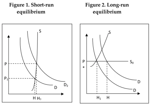
Housing stock depends on depreciated number of dwellings and number of housing completions as in perpetual inventory. It is a common assumption that housing supply is inelastic in the short‐run than in the long run, since housing completions is relatively
smaller than housing stock.(Kenny, 1998) Also Topel and Rosen (1988) explained the reason of this assumption by the high costs of
construction activity when rapid changes occur. So, in the short‐run, the demand for housing driven by the exogenous factors will determine the
price of housing relative to other goods and services.
Figure 1. Short‐run Figure 2. Long‐run equilibrium equilibrium
In Figure 1, for any level of house prices below P1, there is an
excess demand for housing and for any level of house prices above P1, there is an excess supply for housing. From the graph, it is quite clear
that under conditions of short‐run equilibrium, any stimulus to housing demand will result in a rise more in house prices relative to other goods
and services than house dwellings as mentioned in Kenny (1998).
Hence, the microeconomic studies of house market predict a very strong relationship between the arguments of housing demand function
and the real price of housing in the short‐run.
However, in the long‐run, a sudden increase in demand results
again rise in house prices, this time construction firms will find it P P1 S H H2 D D2 P * S0 S D D H1 H
profitable to supply more housing units to the market which makes the supply curve more elastic.
3.1. Housing Supply
Much of the literature has focused on the determinants of new housing supply, particularly the supply of single family detached
homes, and the renovation and repair decisions of homeowners. It has focused on aggregate data because there is so little information where
the unit of observation is the builder, investor, or landlord. In addition,
since housing is a durable good, housing supply is determined not only by the production decisions of builders of new units but also by the
decisions made by owners of housing (and their agents) concerning conversion of the existing stock of housing. (Dipasquale, 1999)
While modeling supply side of the market, Poterba (1984)
assumes that the home‐building industry is composed of competitive firms and that the industryʹs aggregate supply depends on its input
prices and the real market price of housing. Assuming there are limits to supply of any factor of production (such as lumber), increases in
demand for construction increase the equilibrium price of structures.
Poterba defines supply as net investment in structures, ignoring land
prices; he acknowledges the importance of land but omits land in his empirical studies because of the data issues for his empirical work.
A disadvantage of a cost structure based on rising supply price alone is that it does not make the Marshallian distinction, in which the
longer the period, the fewer things that you are holding constant while
you analyze the response of a market to an external shock, between short‐run and long‐run supply responses: the industry supply curve is
fixed, and has no time‐dimension. This assumption gives an industry version of the adjustment cost theory of investment, but is unlikely to
be valid, because supply is likely to be more inelastic in the short‐run.
Therefore, the nature of the short and long‐run supply conditions of factors of production to the industry is specified. Thus, for example,
labor does not move costless in and out of the industry. Neither does capital. Short‐run factor supplies are less elastic than long‐run supplies.
To go in this direction, it requires introducing additional state variables into the analysis, which increases the complexity of the model,
more tractable alternative where supply conditions of factors are
approximately incorporated into an expanded cost function which
includes the rate of change of industry output. Short‐run output supply inelasticity is implied by cost penalties to rapid changes in the level of
construction activity.
A complete model of the dynamics of new housing supply
requires detailed specification of supply dynamics for all factors of
production to the industry. By allowing marginal cost to vary with both the level of output and its rate of change, Topel and Rosen (1988) cut
through the immense complications.
In housing literature, there is a large literature on modeling the
housing supply of new homes. While Topel and Rosen (1988) model the
housing investment under the assumption of perfect foresight, they focus on housing supply. On the supply side of the market, the
representative building firms maximizes discounted profits over an infinite horizon. Since the market is perfectly competitive, profits are
defined as
, İ ,
∞
where P(t) is the price for one unit of housing stock at time t, is gross investment in housing at time t, C represents the costs at time t and is a positive constant representing the interest rate. Furthermore, the industry’s capital evolution equation is 3.1.2 The cost function is specified as , , , 3.1.3 Total cost C at time t is a function of the level of production, the
change in production and a number of cost function shifters represented by a factor y. Note that the inclusion of the change of the
gross investment level is the difference between the cost function in Poterba (1984), who includes only the level of investment, and Topel
and Rosen (1988), who include both the level and the change in gross
investment. Third change in the gross investment level denotes the adjustment cost that the firm faces when changing its output level.
They impose that C is twice continuously differentiable and
that marginal costs are positive and increasing in the level of gross investment I and that the adjustment costs are increasing.
0, 0
/ 0, / 0
Furthermore, the nonnegative constraints for the derivative
cost function (C2 and C22) prevent the infinite production since as the rate of change of investment increases, the cost also increases.
Given these assumptions, we can solve the maximization
problem of the representative building firm by constructing the Hamiltonian equation and taking the first derivatives with respect to , İ
and . The necessary condition for the optimal path is given by Euler equation.
İ
/ İ
3.1.4
If 0, in other words there is no adjustment cost, firms should
choose such that the price equals to the marginal cost. In such a
situation, the right hand side of above equation (3.1.4) reduces to zero and current prices become sufficient in order to determine production.
When the change in İ appears as an argument in the cost
that consists of the right hand side of equation (3.1.4). By the
linearization of euler equation, we can derive,
1 3.1.5
where the terms in and are derivatives of the cost function
evaluated at stationary point, / and / .
If the crucial parameter is zero then the above equation
(3.1.5) tells us that the investment is a function of exogenous cost
shifters and the price.
By rewriting the equation (3.1.5) slightly different, we can
have the following expression,
1 16
where the ’s can be obtained from the equation (3.1.5). In the model
without adjustment costs = 0, that is, changes in exogenous cost shifters are immediately reflected in the level of investment. In the case
where there are adjustment costs ( 0), there is a lag before the new level of investment is reached.
In the literature, Topel and Rosen model is used for different
purposes. Kenny (1999) has considered the potential effects of
asymmetric adjustment costs on the dynamics of housing supply by utilizing from the Topel and Rosen (1988) supply model with the
flexible adjustment costs function advocated in Pfann (1996). His empirical results suggest Irish housing supply is unit elastic in
equilibrium in the long‐run and also in the Irish housing market, adjustment costs associated with an expansion in housing output are
greater than the adjustment costs associated with a contraction.
Furthermore, Kenny (1998) summarizes the housing market in Ireland where his estimations about housing supply and demand is
based on Topel and Rosen (1988) housing models. He also examines the monetary policy developments about Irish housing market by looking
deeply the banking channels and also the inflation policy effects on
housing prices. Topel and Rosen’s (1988) ideas such as the supply restrictions on construction activity are not only used in estimations of supply models but also used in setting up an equilibrium asset pricing model between house prices and rents (Ayuso and Restoy, 2006). They apply their own
constructed model to Spain, UK and US. And they conclude that sharp
increases in house prices lead to price to rent ratios above equilibrium
by mid‐2003 in those countries.
Hakfoort and Matsyiak (1997) examine the determinants of
unsubsidized housing starts in Netherlands by estimating the supply‐
side of the Poterba (1984) model and the supply‐side of the Topel and Rosen (1988) model. The former model yields a supply elasticity of the order 1.6 while the latter yields a short‐ run elasticity of 2.3 and a long‐ run elasticity of 6.
3.2. Housing Demand
Most of the literature for the demand side of the housing market is based on the estimation of price elasticity of demand. As mentioned before, Palmquist (1983) estimates the demand for the characteristic ofhousing by using the hedonic demand theory. He estimates the price elasticity of demand for living space which comes out unitary while the
significant while the expenditure and income elasticities are found to be inelastic. The empirical research for demand differ either in variables used for the estimation or in the method chosen for the estimation. James R. Follain, Jr. (1979) examines the effect of an increase in demand on long‐
run price of housing by finding the price elasticity of the long‐run supply of new housing construction in period 1947‐1975. He shows that
demand function depends on long‐run price of a unit of housing, permanent income of households, interest rate and the price of other
goods. Follain uses real value of private residential construction as a quantity in supply function by applying OLS and TSLS methods.
Dipasquale and Wheaton (1994) estimates demand equation
which is composed of stock of single family units as a function of rent index, age expected homeownership rate, permanent income per
household, price index of single family housing, annual user cost of
homeownership, and total households. They compare two econometric models for actual households as for tenure choice and age expected
households as for both tenure choice and household formation. They find that all elasticities are higher when age expected households are
used than when actual households are used. The regional differences
within a country are seen not only for the supply side of the housing
but also for the demand side of it. Alan K. Reichert (1990) searches effects of some macroeconomic variables upon regional housing prices
by constructing region‐specific housing equations. He derives demand function in the way of assuming utility maximization on the part of
homeowners and wealth maximization on the part of investors. The demand equation is composed of the quantity of new housing sold as a
left‐hand side variable and real housing prices index of new housing quality, resident income, average employment rate, average loan to
value ratio, real mortgage interest rate, the measure of acceleration in
regional housing prices and seasonal dummy variables for each specific region.
In housing economics literature, the demand for housing is
normally derived in multi‐period model where consumers maximize
utility subject to an inter‐temporal budget constraint. These models incorporate various features of housing market including the large cost
of housing relative to the current disposable income and hence the dependence of housing demands the savings in earlier periods and also
Consider a simple demand function which ignores the frictions generated by the heterogeneity of units and the matching of buyers and sellers. (Topel and Rosen, 1988) Under the assumption of perfect capital market, the inverse demand equation of Topel and Rosen (1988) model becomes; 3.2.1
where is the rental price of a housing unit, is a vector of
exogenous demand shifters, be the stock of housing capital and α < 0. There is a perfect foresight deterministic model assumption and taxes are ignored. Then, the rental price of a house is its amortized stock of depreciated price including the interest and capital gains which can be expresses as in the following way; 3.2.2 where r is the interest rate and is the depreciation rate. For explaining this equation in detail, think it as we are in a discrete time. For example, when a household buys a house, the price of a house is the sum of all its rental prices.
3.2.3 where k is the life of a building. In the next period, the price of a house is still sum of the rental prices but there is a depreciation since you did not sell the house in the previous period. Also, you have a depreciated income and income that are exposing to the interest gain. 3.2.4 3.2.5
Equation (3.2.5) is the same with the equation (3.2.2), just written in discrete time. Furthermore, the value of housing stock must
be bounded so that the discounted future price of capital converges:
lim
∞ 0 3.2.6
By taking the integral of equation (3.2.2) with respect to t under the boundary condition, we can write;
∞
Above equation (3.2.7) tells us that the price of a house is the
accumulation of all discounted rental income through its life.
Hence, the complete market dynamics of stocks and prices are described by two linear differential equations:
1 3.2.8
3.2.9
Given the initial conditions 0 and 0 with the boundary
condition (3.2.6), by differentiating (3.2.9) with respect to t and substituting from (3.1.2) yields
1 3.2.10
where .
This demand model (Topel and Rosen, 1988) has its origins in the
work of Walras (1954) and much later by Friedman (1963) and Tobin (1969). They deal with a linear structure for analytical tractability and
present a deterministic (perfect foresight) formulation to illustrate the key ideas. To avoid expository distractions, which are well treated in
the literature, they also ignore the special and peculiar income tax
provisions of home ownership.
This demand part of the Topel and Rosen (1988) model completes the housing supply model since the market should be
thought simultaneously.
3.3 Implications of Theory
Topel and Rosen (1988) housing investment theory provides a framework to analyze the possible determinants of the housing supply
as well as the allowance of short‐run and long‐run analysis in my empirical work. In addition, Topel and Rosen model also contains the
expected present value theory of asset pricing which supports my
empirical analysis and becomes suitable for the Turkish housing market in the way of houses, not being only consumption good but also a part
of a household wealth. Therefore their model is a kind of an extended version of Poterba’s (1984) model.
As in this model, by not omitting the long‐run relations, short‐
run relations can be found and be interpreted in my study with the help
of Vector Error Correction econometric methodology which provides us to study on short‐run dynamics by restricting the variables to converge
to their cointegrating long‐run relations. (Known as Restricted Vector Auto‐Regression).
In my empirical framework, the cost index behaves like one of
the element of the cost function in Topel and Rosen (1988) model, which is denoted as y(t). Because, the cost index has the construction material
prices and in the Topel and Rosen (1988) model the cost shifter is defined as the factor prices that are supplied to the industry, the cost
index can be used as a cost shifter. The other dynamics, represented as gross investment level is composed of the quantity of dwellings,
constructed for the defined period, because the investment level
depends on the change of capital stock with the depreciated capital, equation (3.1.2). Lastly, the rate of change of the investment is added to
the model because of the slow adjustment mechanism of the market in the short‐run, so it is used in the short‐run empirical analysis. In my
empirical framework, the long‐run errors that can be found by Johansen Cointegration econometric methodology and used in the restricted
vector auto‐regression model, and also the first differences of the
variables are the representatives of the rate of change of gross
investment level in the short‐run analysis.
According to the equilibrium equation (3.2.10), when demand
side shifter, , increases under the assumption that the other
variables stay the same, the investment level, , increases since is positive and α is negative. Moreover, as
increases, the capital stock increases. In my empirical study, the demand side shifters are population and income. So as population
increases, the need for houses increases so quantity demanded increases and as income increases, the demand of houses increases. On the other
hand, when the supply side shifter, increases, the price of the investment, , increases then decreases since again
is positive and α is negative. In my empirical framework,
the supply side shifter is the cost index since it includes factor prices affecting the supply and as cost index increases, the desire for building
will decrease due to less profit. Hence, as cost index increases, the level of investment and so the capital stock will decrease. Furthermore, the
α is negative. In this study, the interest rate has also a negative effect on
the quantity of dwellings for both sides of the market. The other
variable, affecting both the demand and the supply, is the price of the investment, . The effect of price to the demand side and to the
supply side is different. According to the supply equation (3.2.8), as price increases, the level of investment increases since is positive and
so the capital stock increases. However, according to the equation (3.2.9), as the price of investment increases, the capital stock directly
decreases due to the fact that is positive and α is negative. The value, which is used as a proxy for the price, has a negative effect on
quantity demanded since as prices increases, less people can buy
houses. However, the value has a positive effect on the supply of houses since building a house may become more profitable than before.
CHAPTER 4
HOUSING MARKET IN TURKEY
Housing was not ranked among the most important socio‐
economic issues in Turkey until the early 1960s. The main reasons for this lack of interest may be summarized as follows. First, the migration
from rural to urban areas was relatively slow and there was no marked deficit in the housing supply at least quantitatively until that era.
Second, the slow pace of industrialization did not make the workers’
housing question an important source of discontent before the early 1960’s. Finally until the beginning of the planned development period,
housing had not been taken up within the broader context of its position relative to the whole of the economy. Therefore, its effect to the
After 1960’s, transition from the traditional family to nucleus
family and rapid rising of population increases the demand for houses,
especially the housing type called apartments which have smaller gardens and more than one floor. Due to Turkey’s problems about
economics such as low level of Gross National Product per capita, chronical high inflation and high interest rates, enough savings for
house building and buying can not be formed. The implemented policies about housing is not efficient enough to solve the problems of
Turkey housing market. In the past, land is allowed to build but the infrastructure is not constructed for a living place, this reduces the
investment desire of the investors. Also, the unavailability of mortgage
credits causes more people not to be able to buy houses for long periods. So, building shanty houses (gecekondu) and unhealthy,
unplanned urbanization spread widely. The promises before each election and frequently accepted construction forgiveness cause to raise
the problem exponentially. (Gurbuz, 2002)
In addition, deficient municipal income is not enough to construct infrastructure services to the new streets and new counties
where there are already lots of shanty houses. Furthermore, deficiency in communication between the municipalities who construct
infrastructure and the utility units who provide electricity and water
causes wasteful expenditure.
Increasing investment to the infrastructure services with the renovation in housing policy in 1980’s maintains the construction sector
to rally. Collective housing fund, housing aid fund to the employees
and especially the Turkey Emlak Bank had assumed the role of the leader for the construction sector. With the guidance of these funds,
house supplies and cooperatives, which are supported by the mortgage credits, increase rapidly. Housing Development Administration of
Turkey starts to build houses for the low income families with facilities in payment. This helps reducing the inequality between demand and
supply in Turkey.
There was seen a significant decline in housing investments in the middle of the 1970’s and also in the beginning of the 1980’s with the
effect of the crisis seen in during 1970’s. Since housing investment is
one of the most important expenditure of a household and it has a high portion in the expenditure of a household, this investment is an
investment increases, especially with the help of government
investment, and then starts to decline in the last years of twentieth
century and in the beginning of twenty first century. By observing the figure 3, we can easily notice that after 1998, the ratio of housing fixed investment to the gross fixed investment is rapidly declining. Figure 3: The share of housing investment in gross fixed investments‐ 1998 current prices
With this decrease investment in housing, Turkey housing
investments is lower than the investment ratios of developed countries, whereas in 1988’s this ratio is near to the developed countries (Eraydin et al., 1996) 0 5 10 15 20 25 30
Housing Investment / Total Investment (% percent)
*Expectation ** Target of the government
The literature about housing in Turkey is widely based on the
inefficiency of the housing policies; little empirical analysis is done due
to the deficiency of data. However, as the housing sector importance is understood, various data collection increases and more studies are
done. For example one of the latest studies is done by Sari, Ewing and Aydin (2007). They investigate the relation between housing starts and
macroeconomic variables in Turkey from 1961 to 2000. They use generalized variance decomposition approach for examining the
relations between housing market activity and prices, interest rates, output, money stock and employment. Their results indicate that the
effect of the housing market on output is not necessarily reflected in
labor market. Moreover, the shocks to interest rates, output and prices have notable effects on housing activity in Turkey.
The provision of housing finance in developing countries is often
problematic, because of the volatile macroeconomic environment and the lack of legal and regulatory framework that supports collateralized
lending. Erol and Patel (2004) evaluate Turkish government’s housing policy for financing the public sector housing and discuss the
be desirable mortgage instruments in periods of persistent high
inflation from the lender’s perspective. The reason behind this finding
is that WIPM eliminate the real interest rate risk, credit risk of adjustable rate mortgages and the wealth risk of the fixed rate
mortgages.
Another research paper on the Turkish real estate market is based on the idea that the housing is both an income decrease for the
tenants and an income provider for the landlords. So housing has some kind of wealth effect for the households that can affect the whole
economy. Binay and Salman (2008) discuss the extent of wealth effects, affordability, financial deepening and credit market risks in Turkish
real estate market. They use price‐ rent ratio to test whether there is a real estate price bubble in Turkey or not. As a result, they do not find
enough evidence supporting that there is a real estate bubble in Turkey,
contradicting what many believe.
Therefore, there is no direct and collective study which is based on formulating both the supply and the demand side of the Turkish
housing market. So, this study aims to determine the factors affecting the housing supply and demand in Turkey.
CHAPTER 5
ECONOMETRIC METHODOLOGY AND DATA
In this chapter, econometric methodology that is found suitable
to use in this study is introduced with the data descriptions. Furthermore, econometric model is briefly explained.
5.1 Methodology
This chapter presents and discusses a brief review of the
empirical methodology employed. In section 5.1.1, we briefly present Phillips Perron Unit Root Tests. In 5.1.2, Johansen Cointegration Test
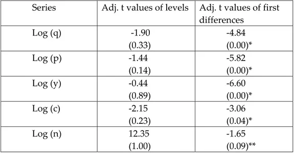
5.1.1 Phillips‐Perron Unit Root Test
A stationary time series has a constant long‐run mean, a finite
variance (time‐invariant) and a theoretical correlogram that diminishes as lag length increases. On the other hand, for a non‐stationary series,
there exists no long‐run mean and its variance is time dependent. Therefore, under the condition of non‐stationarity, to use classical
statistical methods such as ordinary least squares (OLS), usual t‐tests and F‐tests, are inappropriate. However, in order to decide the presence
of unit roots which can be defined as a tendency for changes in a system
to persist, in other words non‐stationarity in a system, only looking at the sample correlogram is unreliable. A formal test to detect the
possible presence of unit roots is developed by Phillips and Perron (1988)
The distribution theory supporting the Dickey‐Fuller tests
assumes that the errors are statistically independent and have a constant variance. In using this methodology, care must be taken to
ensure that the error terms are uncorrelated and have constant variance. Phillips and Peron (1988) developed a generalization of the Dickey‐
Fuller procedure that allows for fairly mild assumptions concerning the
distribution of the errors.
The Phillips‐Peron test is explained in Enders (1995) as follows:
Suppose that we observe observations 1,2,...,T of the {yt}
sequence and estimate the regression equation:
2
Fortunately, the changes are minor; simply replace with , with α, and with β. Thus, suppose we have estimated the regression:
2
where , , and α are the conventional least squares regression coefficients. Phillips‐Perron derive test statistics for the regression coefficients under the null hypotheses that the data are generated by where the disturbance term is such that 0.
There is no requirement that the disturbance term be serially
uncorrelated or homogenous. Instead, the Phillips‐Perron test allows
the disturbances to be weakly dependent and heterogeneously distributed. The Phillips‐Perron statistics modify the Dickey‐Fuller t‐statistics by allowing for an adjustment to account for heterogeneity in the error process.
The appropriate critical values are given in MacKinnon (1991)
same with the Dickey‐ Fuller test critical values.
5.1.2. Johansen Cointegration Test
The sequences {yt} and {zt} are cointegrated, if they are integratedof the same order, let us say d, or I(d), and their residual sequence is stationary. It is a known fact that OLS estimation procedure can be
applied if the variables involved in the model are I(0). The violation of
this assumption causes us to obtain spurious correlation (Granger and Newbold,1974). While dealing this problem, Davidson et al. (1978) state
that fitting the regression by using the first differences of the variables
would result in a loss of valuable information about the long‐run.
Therefore, they propose an error correction mechanism (ECM) by combining the first differences of the short‐run and undifferenced
values of the long‐run dynamics. However, Engle and Granger (1987) prove that this method developed by Davidson et al. (1978) is true if the
variables in the model are cointegrated.
A theoretically more satisfying approach is developed by Johansen (1988) to consider the cointegration relationship when there
are more than two variables. This procedure is explained in Watson and Teelucksingh (2002) as follows; xt is composed of (n,1) vector of I(1)
variables whose vector autoregressive (VAR) representation is given as, Π Π Π ε (5.1.2.1) where Π are (n,n) matrices. It can also be written as, Δ Γ Δ Γ Δ Γ Δ Γ (5.1.2.2) where Γ Π Π Π and
Γ Π Π Π
The purpose of the Johansen procedure can be stated as follows;
1. To determine the maximum number of cointegrating
vectors
2. To obtain the maximum likelihood estimators of the
cointegrating matrix (β) and adjustment parameters (α) for a given
value of r.
The rank of the matrix Γ, r, is equal to the number of
independent cointegrating vectors. There can be at most n‐1
cointegrating vectors and if r=0, it is a known fact that the variables are not cointegrated and equation (5.1.2.2) is VAR model in first
differences. If r=n, the vector process is stationary. For 0<r<n, the Γ matrix can be represented as
Γ ′ (5.1.2.3)
where α and β are full column rank matrices with size (n,r),
,
Equation (5.1.2.2) is denoted as a vector error correction model
(VECM). When there are r cointegrating vectors, r error correction
terms appear in each of the n equations. For instance, in the first equation (explaining ∆x1t ), αβ’xt‐1 consists of terms,
′ ′ . . ′
It is known that the number of cointegrating vectors is equal to the number of significant characteristics roots of the matrix Γ. Suppose
the ordered characteristic roots of the matrix Γ are; . To obtain the number of characteristic roots that are different from zero,
Johansen proposes the following tests, that are based on trace and maximum eigenvalue statistics, respectively, ∑ ln 1 (5.1.2.4) , 1 ln 1 (5.1.2.5) where is the estimated values of characteristic roots (eigenvalues) of the estmated Γ matrix and T is the number of usable observations.
The trace statistic tests whether the number of cointegrating vectors is less than or equal to r against a general alternative while the
alternative hypothesis for maximum eigenvalue statistic is r+1. The critical values for these statistics are calculated by Johansen and Juselius (1990) with the help of simulation.
5.1.3 Vector Error Correction Model (VECM)
A vector error correction model (VECM) is a restricted VAR
designed for use with nonstationary series that are known to be cointegrated. The VEC has cointegration relations built into the
specification so that it restricts the long‐run behavior of the endogenous variables to converge to their cointegrating relationships while allowing for short‐run adjustment dynamics. The cointegration term is known as the error correction term since the deviation from long‐run equilibrium is corrected gradually through a series of partial short‐run adjustments.
Formally, the (nx1) vector , , … , ′ has no error‐
correction representation if it can be expressed in the form:
Δ Δ Δ Δ (5.1.2.6)
π0 = an (n x 1) vector of intercept terms with elements πi0
πi = (n x n) coefficient matrices with elements πjk(i)
π = is a matrix with elements πjk such that one or more of the πjk ≠ 0
= an (n x 1) vector with elements
Note that the disturbance terms are such that may be correlated with
The key feature in (5.1.2.6) is the presence of the matrix π. There are two important points to note:
1. If all elements of π equal zero, (5.1.2.6) is a traditional
VAR in first differences. In such circumstances, there is no error‐ correction representation since Δxt does not respond to the previous
period’s deviation from long‐run equilibrium.
2. If one or more of the πjk differs from zero, Δxt responds to the previous period’s deviation from long‐run equilibrium. Hence,
estimating xt as a VAR in first differences is inappropriate if xt has an error‐correction representation. The omission of the expression πxt‐1