Entropy Solution of a First Order Hyperbolic Type Equations with a Non-Convex State Function in a Class Of Discontinuous Functions

>

ENTROPY SOLUTION OF A FIRST ORDER HYPERBOLIC TYPE EQUATIONS WITH A

NON-CONVEX STATE FUNCTION IN A CLASS OF DISCONTINUOUS FUNCTIONS

Mahir RESULOV* , Ethem Ilhan SAHIN**

*Beykent University, Department of Mathematics and Computing, Istanbul, Turkey, [email protected]

**Yildiz Technical University, Department ofPhysics, Istanbul, Turkey [email protected]

ABSTRACT

In this paper, a method for obtaining an exact and numerical solution of the Cauchy and first type initial boundary value problems for a first order partial differential equation with a non convex state function is suggested. For this purpose, we introduce an auxiliary problem since it has some advantages over the main problem, and it is equivalent to the main problem in a definite sense. Using this auxiliary problem, we propose a efficient method for finding the location of shock which appears in the solution of main problem and its evolution in time. The suggested auxiliary problem permit also us to prove of convergence in mean of a numerical solution to the exact solution of the main problem. Moreover, using the auxiliary problem we can write the higher order numerical scheme with respect to the time variable. Some results of the comparison of the exact and numerical solutions are illustrated.

Keywords: Riemann's and Buckley-Leverett's problems, non-convex

state function, convex and concave hull, numerical solution in a class of discontinuous functions

ÖZET

Makalede sabit katsayılı adi diferansiyel denklemler sistemi için yazılmış Cauchy probleminin rezidü metodu ile gerçek çözümü elde edilmiş ve söz konusu metot uygulanarak sabit gerilimli bir RC devre probleminin çözümünün bulunması için uygulanmıştır.

Anahtar Kelimeler: Riemann ve Buckley-Leverett problemleri, konveks

1. INTRODUCTION

The theoetical investigation of many important problems of physics and engineering are reduced to finding the solution of a first order hyperbolic type equation as

du dF(u) n — + — — = 0

dt dx

with corresponding initial and boundary value conditions.

(11) It is well known that the equation (1.1) is the model equation of gas dynamics and has been used to model various problems of hydrodynamics, [1], [2], [9], [11], [26], [28]. It has been proven that, (see, for example, [3], [8], [12], [15], [18], [26], [28]), the solution of the equation (1.1), becomes multi-valued if the initial profile has both a positive and a negative slope. Similar features appear in the solution of the Riemann problem too. Since a multi-valued solution has no meaning from a physical point of view, (see,

[9], [12], [14], [18], [26], [28] ) the necessity arises to extend the concept of a classical solution and propose a method for obtaining a single-valued solution (weak solution) which may have discontinuities with finite jumps.

The solution obtained by using the method of characteristics has an implicit form as

u(x, t) = f ( x - F'(u)t), ₍₁₂₎

where f is any differentiable function. But, from this expression, it is often impossible to obtain an explicit formula for the unknown function. We will call the obtained functional relation (1.2) as the alternative form of the equation (1.1).

The existence of the points of discontinuities in the solution of (1.1) makes it vulnerable to the numerical schemes, due to the fact that near a point of discontinuity, a finite difference approximation to the first-order derivatives yields rather poor results.

Various finite difference methods have been applied to find the solution of the Cauchy problem for equation (1.1) (see, for example ([2], [3], [4], [11], [16], [15], [19], [24], [25], [27]).

In the literature, there are also such homogeneous finite differences schemes that ignore the jump points which appear in the solution. It is known that the classical finite difference schemes when applied to (1.1) the so-called numerical viscosity appears in the equation. Such numerical viscosity has a negative effect on the solution. More precisely, it causes the numerical propagation rate of the wave to be larger than the actual physical rate. Furthermore, there exist some other numerical methods that employ the method of characteristics, see [5], [6], [10], [11], [24], [25].

When we include the concept of a weak solution, a new problem arises, as the location and time of the discontinuous points become unknown. It is obvious that a weak solution defined for nonlinear differential equations automatically fulfills the known jump condition. However, this statement is not valid for the soft

solution [17].

The concept of a weak solution has been employed extensively in obtaining differences approximation for the equations of hydrodynamics. P. Lax showed [14] how it can be used for numerical computation and Lax & Wendroff [15] showed that the entire classes of difference methods lead to solutions which converge to weak solutions of differential equations. However, having finite difference solutions converging to the weak solution of the hydrodynamics equations does not permit to approximate the hydrodynamics equations by finite difference methods. As it is shown in [3], when we approximate the equation (1.1), when

u 2

F (u) = — , by the finite difference method, we do not obtain the

solution for the equation (1.1), in fact, we obtain the solution for the modified equation below

ut + uux = hu^, (13)

where h is the grid size.

We emphasize that the solution of the equation (1.1) has unknown points of discontinuities, and the equation (1.1) can not be approximated by the finite differences method. Furthermore, the principle of causality is violated. That is, when we directly approximate the equation by the finite differences method we

artificially take the wave to a point which it has not physically reached. This approach leads us to the wrong solutions.

Equation (1.3) is called Burgers's equation and it includes the diffusion and the convection effects. G.B.Whitham showed in [28] that, if the diffusion term is small enough it removes the effect of the convection term which leads to a continuous solution. This in fact corrupts the physical structure of the problem.

In the case where the initial function is piecewise constant or, in general, if u(x,0) e Lx(R2) and F''(u)>0 ( or F"(u)<0) then

it is noted that (see, [12], [14], [16], [26], [28]) the Cauchy problem has multi-valued solutions from which the physically efficient solution can be obtained by imposing the so-called entropy condition. In [8], [13], [14], [16], [18], [26], [27], [28], under the assumption that F (u) does not change sign, a method for obtaining the extended solution satisfying the entropy condition is proposed.

In this study, we consider the Cauchy and first boundary value problems for a one-dimensional first-order nonlinear wave equation and propose a method for obtaining the exact and numerical solution in a class of discontinuous functions when

F (u) has alternative sings. Unlike the classical schemes, the

proposed scheme does not require regularity assumptions on the unknown function and remains valid for higher dimensions.

2. THE EXACT SOLUTION OF THE CAUCHY PROBLEM

As usually, let R2(x, t) be the Euclidean space of points

(x, t). We denote Q ={x e R \ 0 < t < T} c R2(x, t), here

R1 = ( - w , <x>).

In this section we will construct the exact solution of the equation (1.1) with the following initial condition

u( x,0) = uo(x), (2.1)

and investigate some properties of this solution. Here, u (x) is a known measurable and bounded function in particular case with compact support having both a positive and a negative slope.

Suppose that the function F(u) is known and satisfies the conditions:

• F(u) is a twice continuously differentiable and bounded

function for bounded u ;

F'(u) > 0 for u > 0;

• F''(u) is a function with alternating sings i.e. F has convex

and concave parts.

2.1. Continuous Initial Profile

A solution of the problem (1.1), (2.1) can easily be constructed by the method of characteristics [1], [8], [9], [11], [12], [13], [14], [16], [26], [27], [28] and it has the form

here,

u( x, t ) = u,(£),

^ = x - F (u)t

(2.2)

(2.3) where, i is the spatial coordinate moving with speed F'(u).

From (2.2), (2.3) we have du(x, t) _ u'(i) Sx (1 + u' (i)F''(u)t)' du(x, t) _ u' (i)F'(u) dt (1 + u0(£)F'' (u)t) (2.4) (2.5) Relation (2.4) expresses the slope of the profile u( x, t) at the point (x, t) in terms of the slope of the initial profile at

(x = i , t = 0) . If u' < 0 and F' '>0, or ( u' > 0 and F'' <0 ) then

for t = • -1

<(£) F' '(u) we have ux (x, t) = » . At these points ut (x, t)

also becomes infinite. Therefore, the problem (1.1), (2.1) does not have a classical solution.

Definition 1. The function u(x, t) satisfying the initial

condition (2.1) is called the weak solution of the problem (1.1), (2.1) if the following integral relation

\\Q fa (x, t)u(x, t) + çx (x, t)F(u)}dxdt + J u(x,0)ç(x,0)dx = 0 (2.6) holds for every function (p(x, t), which is defined and twice differentiable in the upper half plane and which vanishes for sufficiently large t + | x |.

2.2. The Auxiliary Problem

In order to determine the weak solution of the problem (1.1), (2.1), in accordance with [20], [21] the auxiliary problem

M f b

v(x,0) = V0(x) (2.8)

is introduced. Here, v (x) is any absolutely continuous function satisfying the following equation

dvn (x) . s

—T^ = u0( x). (2.9) dx

Theorem 1. If v(x,t) is a solution of the auxiliary problem

(2.7), (2.8), then the function u( x, t), defined by

u(x, t )= (2.10) Sx

is the soft solution of the main problem (1.1), (2.1).

Suppose that v(x, t) is a solution of the problem (2.7), (2.8). We introduce the following notations

Sv Sv — = p, — = q.

St Sx

Using these notations the equation (2.7) is written as

Differentiating the last equation with respect to x and t, we have

dp + Q dq =0^ dp + Q dq = ^ Sx Sx St St

here, Q = — . Noting that — = — , for the unknown variability

Sq Sx St

characteristics in the space (x, t, v, p, q), we get

dt dx N dp „ dq ^ dv ,—. .

-- = 1, — = F (q), -f = 0, -dq = 0, — = p + F (q). (2.11)

ds ds ds ds ds

The system (2.11) uniquely determines x, t, v, p and q as functions of s provided their initial values are known. The initial conditions for the system (2.11) at s = 0 are given in the form

K , I ;I * I , t \s=0 1, x \s=0 g, v \s=0 I „ I r I . , , { 0 \ g \> 1 v\ = a\ = = \Uo, \g\*1 pls=0 F l a x J als=0 dx 1 0 , \ g \>1. (2.12) The solution of the problem (2.11), (2.12) can easily be obtained, and has the form

v( x, t) = d v.F' [dv V F[ d v

dx l dx dx t + V0(g), (2.13)

/ d v0

t=

-F

lax-

/

By calculation, it can be easily shown that u(x, t ) = X't ).

dx

It is also easy to see that an integrable soft solution is a weak solution [17], that is, the following theorem holds.

Theorem 2. If v(x, t) is the solution of the auxiliary problem

10. the function u(x, t) defined by (2.10) is the weak solution

of the main problem;

20. v(x, t) is an absolutely continuous function. The auxiliary solution has the following advantages:

• The function v(x, t) is smoother than u(x, t) ;

• u(x, t) can be determined without using the derivatives

Su Su

— and — , which are not defined at the neighborhoods of the

Sx St

points of discontinuities.

According into consideration (2.10) the equation (2.7) can be rewrite in the form

fxu(g, t )dg + I[F (u(x, T)) — F (u(r, T))\-T = 0, (2.14)

Jr J0

here r is any real number r e (—w, w).

2.3. Shock Fitting

In order to obtain the location of the points of discontinuity which arise in the solution of the main problem we will use the

/ • w

facts that I u(x, t)dx = const, and that this integral exists not only

J—w

for multi-valued and continuous functions, but also for single-valued piecewise continuous functions. In addition, it is known that the equation (1.1) expresses the conservation law of mass. Let

E (t) denote the following integral

E (t) = \u(x, t)-X .

Definition 2. The number E (0) , defined by E (0) = \u( x,0)dx

is called the critical value of the function v(x, t).

Now we investigate the problem of finding the locations of discontinuous points of u(x, t) and the time evolution of these points. As it was expressed before, the solution of an auxiliary

problem is not unique. Some additional conditions are required in order to find a physically meaningful and unique solution.

Definition 3. For every t, the geometrical location of the

points, where v( x, t ) takes a critical value is called the front curve. Let x/ = Xy (t) be the equation of the discontinuity curve of

v(x, t) . Considering Definition 3 and expression (2.10), we have

v( x, (t ), t )= f Xfu( x, t )dx = E (0).

f J—œ

From the last relation we have

dXf (t)_ [F(u)]. _{dt [u\} x=xf( t ) ' (2.15)

Here [f \ shows the shock of the function f at a point x = x0, i.e.

[f \ = f (x0 + 0) — f (x0 — 0).

Definition 4. The function defined by 'v(x,t), v < Ei(0),

ve x t(x t ) = '

Ei(0), v > Ei(0)

is called the extended solution of the problem (2.7), (2.8).

From Theorem 1, for the weak solution of the main problem (1.1), (2.1), we have

u „ ( x, t ) = _Sx ^ .

This means that a point of discontinuity for u( x, t) is one to the right of which the solution of the problem (1.1), (2.1) is equal to zero.

From (2.15), we easily obtain

dxf (t)

dt

F (u)N

hence, t = f f

J o

xf (t) dx

F (u)

Thus the necessary and the sufficient condition for the existence of a jump for u(x, t) is that the integral

rx_ff _{< ^} (t) dx Jo F(u)

, • v(x, t) - v(x - a, t) „

Now we consider the relation for any

a a > 0 v(x, t) - v(x - a, t) _ 1 ft a a | [F (u( x, r)) - F (u(r, r))]dr < 1 rT E - [ [F(u(x,r)) -F(u(r,r))]dr < -l, (2.16) aJ 0 t 2

here -1=— s u p F(u). This is the entropy condition in sense

a

Oleinik, (see, [18], which show the rate of spreading of characteristics. Hence v(x, t) is the entropy solution to the problem (2.7), (2.8).

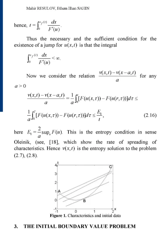
Figure 1. Characteristics and initial data

3. THE INITIAL BOUNDARY VALUE PROBLEM

In the previous section we found the solution of the Cauchy problem for first-order nonlinear equation of the hyperbolic type. But, many important practical problems such as the displacement of fluid by water in a porous medium, the traffic flow problem etc.

are expressed by the initial boundary value problem for the mentioned equation [7], [16], [19], [21], [23].

Suppose that the solution of the equation (1.1) is given on a curve i = i(t) in a plane (t, x). It is known that, [11], [21], [28], if

the characteristics of the Eq. (1.1) intersect this curve once, then the solution of the equation (1.1) is determined uniquely, and this is called a Cauchy problem. In other words, from the trace of the solution on the initial curve, the solution may be determined in the entire region which has been covered by the characteristics of the Eq. (1.1).

If the characteristics of the equation (1.1) intersect the given initial curve twice, as shown in Fig. 1, than we give the initial condition either on the AB or the BC curve. Otherwise, the solution defined on the curve AB and the one defined on the curve

BC do not match. Since the slope of the characteristics of the

equation (1.1) depends on the solution, usually, it is not possible beforehand to know the region covered by the characteristics of the equation (1.1) where the boundary conditions are given.

The typical initial boundary value problem describing the distribution of some signal in D = {x > 0 , t > 0} is

du dF(u) _ St dx u( x,0) = u( x), (3.1) (3.2) u(0, t) = u (t). (3.3)

Here, u0 (x) and u (t) are given functions, and u (0)> u0 (0). It is obvious, that the solution of the problem (3.1)-(3.3) may be connected with solutions of two Cauchy problems, for any F (u) function, when F'(u) > 0. We introduce the following Cauchy problems:

du dF(u) _ dt dx u( x,0) = u0( x);

du dF(u) n + — = 0,

dt dx u(0, t) = u (t ).

The exact solution of the main problem (3.1)-(3.3) was constructed in [21], [23], [28], and has the form

u( x, t ) = u0(£l x ~> F'(uo), G(X), F'(uo)< X < F'(u), (3.4) ui(j) ~ < F'(ux).

here G(g) is the inverse function F' (u) over [u0, u ] .

As noted in [21], [23], and [28] the solution (3.4) is a multi-valued function for any x > 0 and t >0 .

The weak solution of the problem (3.1)- (3.3) is defined as.

Definition 5. The function u(x, t) and satisfying the

conditions (3.2),(3.3) is called the weak solution of the problem (3.1)- (3.3) if the following integral relation

j j {f (x, t)u + fx (x, t)F(u)}dxdt + Jo u(x,0)f (x,0)dx

+ jTF (u(0, t)) f (0, t)dt = 0 (3.5)

J0

holds for any test functions f (x, t) for which f ( x , T ) = 0. In order to obtain the weak solution of the problem (3.1)-(3.3) in sense of (3.5), according to [21], [22], the following auxiliary problem, known as the first kind auxiliary problem

dv(x, t) | J dv(x, t) ^ = Q dt 1 dx , v ( x , 0 ) = vo( x ) (3.6) (3.7) <

dv(0, t) dx

is introduced.

= ul ( t ) (3.8)

It is note that, the Theorem 1 is valid for the problem (3.6)-(3.8). As is obvious from Eq.(3.6), in this case the function u(x, t) may be discontinuous, too. Besides, the auxiliary problem allows us to write economical and efficient higher-order finite differences schemes for obtaining the solution of the problem (3.1)-(3.3). The solution of the problem (3.6)-(3.8) is

v0(£) + [u0(g)F'(u0(g)) - F (u0(m, ~> F' (u0(&), v( x, t ) = < UT - F(_{F (u (t))}Ul(J}l x-\f (ul(rl))drl, J0 F'(uo)< f < F'(u),(3.9) y < F' (u).

The exact solution of the problem (3.6)-(3.8) was investigated in detail in [21], [23].

In order to is constructed the weak solution of the problem (3.6)-(3.8) we may be to use the second kind auxiliary problem as

3 rx

-j0u(g, t)dg = F(u (t)) - F(u(x, t)), (3.10)

u(0, t ) = u0 (x). (3.11)

let us define E (t) as

E(t) = jXu(g, t )dg = £ [ F U (0)) - F (u( x,0))]dz, (3.12) and

'v(x, t), v(x, t) < E(t),

vext(x, t) = j (3.13)

ue x t( x>t ) = <

foext(x, t ) ,

dx v(X, t) < E(t), v( x, t )> E (t ).

(3.14)

Taking into consideration (2.10) and (2.14), for value of

t > 0 and a > 0 we now consider

v(x, t) - v(x - a, t) _ 1 f fV a — ( u ( x - a, r)) - F(u(x, r))]^r} < 1 t E 1 {ï [F(u(x - a, r)) - F(u(x, r))]rfr} < E 1, J0 / a

here E1 = 2 sup F (u)

a and t < T. Hence the solution of the problem (2.10), (2.11) is the entropy solution.

4. FINITE DIFFERENCES SCHEMES IN A CLASS OF DISCONTINUOUS FUNCTIONS

In this section, using the above introduced auxiliary problem we develop a numerical method to solve the problems (1.1), (2.1), and (3.1)-(3.3) and investigate some properties of the numerical solutions.

4.1. The Finite Differences Scheme for the Cauchy Problem

In order to construct the finite differences method, at first the domain of definition of the problem is covered by the following grid

= {( x, h ) | x = ih, h = kr, i = 0+1+2,..., k = 0,1,2,...; h > 0,r > 0}

h,r

where, h and r are steps of the grid for x and t variables, respectively.

The problem (2.7), (2.8) is approximated by the finite differences scheme at any point (i, k) of the grid coh r as follows

V, k+—= V, k -rF

Vi, 0 = V0( x ).

( V, k - Vi-—k 1

h (4.1)

(4.2) A function v (x ) is any solution of the following finite differences equation

(Vo)xx = ua(xt). (4.3)

It is easy to prove that U k+— =

V - V

V i,k+— Vi-1,k +—

h (4.4)

Here, the grid functions U k and Vik represent approximate values

of the functions u(x, t) and v( x, t) at point (i, k) respectively. In order to prove (4.4), firstly we write the equation (4.1) at a point (i - 1 , k), then subtract it from (1.1) and divide by h. By taking (4.4) into consideration, it is seen that Uik satisfies the

following nonlinear system of algebraic equations

Uh k+ — = U h k - L ( F ( U i , k ) - F UU-—,k )). (4.5)

h

Initial condition for (4.5) is

U,o = u0(xt ). (4.6)

Theorem 3. The expression E,(tk ) = hJUhk

i

is independent of time, that is h y Ui k + i = h y Ui k.

Proof. Multiplying (4.5) to h and summing with respect to i, we get

This means that E t ) is independent of k. This completes the proof.

Definition 6. The quantity E (0) defined by E1(0) =

i

is called the critical value for the grid function Vik.

Definition 7. The mesh function defined by

Vik, Vik < E(0),

V T = <

E(0), Vik >E(0)

is called the extended solution of the problem (4.1), (4.2). From Theorem 1, we have

ux=(vTh,

and this expression is called the extended numerical solution of the main problem.

As it can be seen from (4.1), (4.2), the suggested algorithms are very effective and economical from a computational point of view.

The finite differences analogy of the (2.14) is

i k

hTP^ = tYJlF (U„) - F (UhV)], (4.7)

j=1 V=1

here q is such number for that the r = (i -q)h is valid. Let us p is any positive integer, and consider

V, -V , 1 K K

IK L-P,K =-{Tj}_F(Uqv) - F (Uiv)] -

TY[[F(U

)

p p v=1 v=1

1 k 1 .f —

-{TYJlF (U- J - F (UJ] < - J [F (u(x - a, t) - F (u(x, t)]dt < - f , (4.8)

2

where a = (i - p)h and E2 =— max uF (u). Therefore, the

P

numerical solution of the problem (4.1), (4.2) satisfies the entropy condition too.

Additionally, considering (2.10), we rewrite (2.7) as

dv( x, t)

dt + F (u( x, t )) = 0.

Then, by applying for example, the Runge-Kutta method to the equations above, we can write a higher-order finite differences scheme for the main problem with respect to r .

4.2. The Finite Differences Scheme for the Boundary Initial Value Problem

The finite differences analogy for (3.6)-(3.8) is V,k+1= V,k - F Vo = v0( X) , v - V V 1,k v 0,k \ - " — j k = U1(tk ). h f v - V ^ v i,k vi-1,k h (4.9) (4.10) (4.11) It is easily show that the equality (4.4) is fulfilled for the problem (4.9)-(4.11). As above the extended solution for the problem (4.9)-(4.11) is writed in the form

^ e x t(X t )= 1

V,k, Vuk < E3(tk ),

E,(tk), V,k > E3(tk),

(4.12)

here E3 (tk ) = [F(u (0)) - F(u(x,0))]. Using the Theorem 1 we can find the extended numerical solution of the main problem (3.1)-(3.3).

We can write analogies estimate to (4.8) for the solution of the problem (4.9)-(4.11), i.e, for the in question solution entropy condition is satifies.

In order to find as a matter of fact the numerical solution of the problem (3.1)-(3.3), we will use the second kind auxiliary problem which is equivalent to (3.1)-(3.3). But then, the point in question auxiliary problem (3.6)-(3.8) is convenient tool as theoretical investigations of by proof of convergence of the numerical solution to the exact solution of the main problem, and by study of a some theoretical property of the solution.

Firstly, we approximate the integral included in (3.10) by

t d = hfUjk.

j=1

(4.13) By taking into account, (4.13) for the equation (3.10) we will write two kinds of difference schemes:

1) explicit scheme

T ' -1

Uk+1 = Uuk + -[F(Ui(tk)) - F(Uhk)] - YjUhk+1 - Ujk). (4.14)

n j=i

The system of equations (4.14) is solved under condition (4.6). This differences scheme is simple and to obtain the solution

from (4.14) does not present any difficulty. But this scheme

U j,k+1

requires the severe constraints on the steps of grid. In order to flee from this limitation we will write 2) implicit scheme

i-1

U,k k+1 = U,k +-[ F (Ui(tk+1)) - F (Uhk+1)]-Z(Ujk+1 - Ujk k). (4.15)

j =1

The differences scheme (4.15) is nonlinear with respect to

U . For finding this solution we can be apply following scheme:

a) simple iteration

Ul:;H= Uik +^[F(u1(tk+1)) - FUS+1)]-lPCl+1 - Ujk). (4.16) b) Newton iteration

j=1 i-1

T i-1

U S = Uhk + T[F(Ui(fk)) - F ( U ™ ) ] - Y j U j l+1 - Ujk). (4.17) j=1

To obtain the solution we represent it in form

u( s + 1 ) = U( s ) +S U( s ) uk + 1 U. ^ i + U U J i Itmi.

Substituting the last relation in (4.17) and linearizing it, we have

i - 1

Uk+1 = -ZUk+1 - T F '(U^tUCL+U, k+1 U(5+1)

-j=1

- h F ( U S + i ) - U M ) ik+1). (4.18)

It is obvious from (4.18) that this algorithm is economical and efficient from a computational point of view and it permit us to find the solution SU(j+1 easily.

4.3. Consistency and Convergence

Now we will show that the difference scheme (4.5) is monotone. For this, (4.5) let us rewrite in form

U k+1= H U-hk,Uh k )

where ^ U ^ U ^ ) = U^k +T (F(U^) - F(UIJc)).

h It is

obviously that if

0 < - F ' ( U ,) < 1 then > 0

h ( k) dUjkk

for ( j = i — 1,i). Hence, if the CFL condition is fulfilled, then the difference scheme (4.5) is monotone. The definition of a monotone scheme is actually equivalent to the following property;

if Wt k > Ui k for any i then W k+1 > U, k+1- (4.19) Theorem 4. Let ( Uk) be given set, if ( Ui +J is solution set

founded with a monotone scheme (4.5) then

max{U, k+1 } < max{Ui ,k}; ^or min{Uhk+i} > mm{Uhk(4.20) Proof. Let Wik = m a x, { Ut k} for any i. From (4.5) we have

Wk+ i = W. , . As W^k > Uuk, application of (4.19) gives

W,k+i= Wi,k > Ui,k+i a n d t h e f o r e maxi{Uhk+i} < max,{Uhk}. T h e

second inequality in (4.20) follows similarly. From (4.20) also follows

max { U, ,k } < max {U,,k-i} <... < max { U,,0 } , min {U,,k} > min {Ut k_} >... > min {Ut o}.

It is easily shown that the differences schema (4.9) is monotone, too. In deed, under the CFL condition

j, ( j = i _1 , i) here, / \ f V _ V ^ H1(VI_1JC,VIJC) = Vhk _TF . I h J SH1 ÔV, _j,k > 0 for any

Let sik and 5ik be the errors of the approximations by the

„ , , . dv(x,t) , dv(x,t) _

differences of the derivatives — : and —: . Then (2.7) can

ôx ôt be written as V k + F {vxx +eu k ) =0 or vt + F (vx ) =Vi, k , W h e r e 1,k = Si,k + F'( Vx )Si,k. (4.21)

Now we will show that the difference schema (4.21) is consistent. It is known that the suitable characteristic of continuity of the function f ( x ) on the any [a,b] is it a module continuity

« ( J , f ) = n ( f ) = sup \ f ( t ) - f ( x ) \ .

At first, we will show that ei k ^ 0 and Si k ^ 0 if the steps

of grid approach to zero. In deed, due to u(x, t) is continuous £

.,k

k

*

k

F'(u)(u(xi, tk) -u(xi,i*)) = F ' ( u ) x ( u ) ^ 0, A e ( tk • tk+1X ~ e ( u ( xi • tk X u ( xi • tk

hence, r]jk^ 0.

Subtracting (2.7) from this equality and writing wik for Vk - Vk, we have the following problem for wik

W + F' ( u ) wx = Vt,k, (4.22) Wi , 0 = JoJ ^ ) ^ - h Y u 0 ( x j ) = w f = O(h) ^ 0, (i = 1,2,..,) U0 ( j=1 w1 , k - w0 , k = hs0,k = O ( h ) ^ 0. According to Theorem 4, = vi , k- ^ 0 , (4.23)

Now, let us multiple the (4.22) to w- and sum with respect to

i, k over grid co^h ,

( wx, w t ) L 2 h ) + ( w x , F ' ( u ) w x ) L 2 h ) = ( wx , Vi,k )L2(mr h). or (R k , F (u) Rh k ) l2 ) = ( w. , k, Rt) L2 ( vt h) + ( R k ,k ) L2 ( vt h) < K k | L M (a ) + W „ L b ' A (n v (4.24) 11 ' "L2(mT,h ^ L2(mT,h) 11 ' nL2(0\,h ) N ' HL2(mT,h) H e r e , t h e n o t a t i o n s Rik = uhk - Uhk a n d ( f , g) h (^ h) i s

differences analogy of the inner production of the functions f and

g, t h a t i s ( f, g ) h ) = ^ f(x)g(x)dx.

From last inequality it is seen that u converges to U with the weighted F'(u) in the sense of L2( aT h) .

5. Numerical Experiments

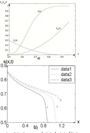
We simulate the experiment which was done in the Department of Phisyco-Chemistry of Porous Medium of the Institute for the Study of Problem of Deep Oil and Gas Deposits, of the Azerbaijan Academy of Sciences.

In this experiment, a cylindrical pipe filled with unfiltered quartz sand is used as the porous medium. The length and cross section of the pipe are given as l = \.2m, S = 9.6-\0 Am2, respectively. The permeability coefficient, k, is 2.22^m2, and the

porosity (m) is 0.298. The transformer oil is used as the fluid model of which the viscosity is 47.9sP, and the surface tension between the water and the fluid is 37 fjNIm. The pipe from one end is attached to a water source whose gradient pressure Ap is

0.03mPa. The amount of connate water in the model is specified

as (s0) 0.23. The duration of the experiment is 54 hours.

0.4 b ) 0.i

Figure 2: a) The graphs of the functions kc (s), kw (5), F(s);

b) Time evaluation of the exact solution a(x, t) 1) T = 105 sec, 2)

T = 1.5 -10s sec, 3) T = 2 -10s sec

The relative phase permeabilities and the Buckley-Leverett function are given, as follows

ko (s) = 0.29 (0.9 - s)2

0.16 kw (s) = (0.5 - 0.00187) (s - 0.5) _0.14 :

F (s) = - kw (s) K ( s ) + Mko ( s )

The graphs of the functions ka (s), kw (s), F (s) are given in

According [7], [23] this experiment is modeled bu the following problem

m * + w(t) ^ =

dt dx

s(x,0) = s0 = 0.23, s(0, t) = s = 0.77

The graphs of the numerical solutions obtained using the algorithm (4.14) are given in Fig.2b at values T = i05sec. ,

T = i.5-i05sec. and T = 2-i05sec., respectively. As it is shown in

Fig.2b, the time of complete displacement of water is approximately 54 hours. Judging from Fig.2b, it is possible to claim that the results obtained from the theoretical problem and the experimental model match quite well.

6. Conclusion

In this study an original method for obtaining the exact and the numerical solutions of the initial and initial-boundary value problems for one dimensional nonlinear partial differential equations in a class of discontinuous functions is suggested. The obtained results are as follows:

The exact solution of the initial value problem with a non-convex state function is obtained when the initial profile is a continuous.

An original method for finding the jump which appears in the solution is developed and its time evaluation is studied.

It is shown that the solutions of the investigateg problems satisfy the entropy condition in Oleinik sense.

Convergence of the numerical solution to the weak exact solution of the main problem is proved.

The higher sensitive differences scheme whose solution accurately expresses all the properties of the physical problem is suggested

The numerical solution of the Bucley-Leverett problem, which describes the macroscopic flow of the two phase fluid in a porous medium is obtained.

REFERENCES

[1] Ames, W.F. Nonlinear Partial Differential Equations in Engineering, Academic Press, New York, London, 1965. [2] Ames, W.F. Numerical Methods for Partial Differential

Equations. Academic Press, New York, 1977.

[3] Anderson, D. A., Tannehill, J.C., Pletcher, R. H. Computational Fluid Mechanics and Heat Transfer, Vol. 1,2, Hemisphere Publishing Corporation, 1984.

[4] Bakhvalov, N.S., Jidkov, N.P., Kobelkov, G.M. Numerical Methods, Moskow, Nauka, 1987.

[5] Courant, R., Lax, P. On Nonlinear Partial Differential Equations with Two Independent Variable, Comm. On Pure and Applied Mathematics, vol. 2, No.3, pp. 255-273, 1949. [6] Courant, R., Isaacson, E., Rees, M. On the Solution of

Nonlinear Hyperbolic Differential Equations by Finite Difference, Comm. On Pure and Applied Mathematics, vol.5, pp. 243-255, 1952.

[7] Collins, P. Fluids Flow in Porous Materials. 1964.

[8] Debnath, L. Nonlinear Partial Differential Equations. Birkhauser. Boston. Basel. Berlin, 1997.

[9] Fritz, John. Partial Differential Equations, Springer-Verlag, New York, 1986.

[10] Godunov, S.K., Ryabenkii, V.S. Finite Difference Schemes. Moskow, Nauka, 1972.

[11] Godunov, S.K. Equations of Mathematical Physics. Nauka, Moskow, 1979.

[12] Goritskii, A.A., Krujkov, S.N., Chechkin, G.A. A First Order Quasi-Linear Equations with Partial Differential Derivatives. Pub. Moskow University, Moskow, 1997.

[13] Krushkov, S.N., First Order Quasilinear Equations in Several Independent Variables, Math. USSS Sb., 10, pp.217-243,

1970.

[14] Lax, P.D. The Formation and Decay of Shock Waves, Amer. Math Monthly, 79, pp. 227-241, 1972.

[15] Lax, P.D. Weak Solutions of Nonlinear Hyperbolic Equations and Their Numerical Computations, Comm. of Pure and App. Math, Vol VII, pp 159-193, 1954.

[16] LeVeque R.J. Finite Volume Methods for Hyperbolic Problems. Cambridge University Press, 2002, 558p.

[17] Noh, W.F., Protter, M.N. Difference Methods and the Equations of Hydrodynamics, Journal of Math. and Mechanics, Vol. 12, No. 2, 1963.

[18] Oleinik, O.A. Discontinuous Solutions of Nonlinear Differential Equations, Usp.Math. Nauk, 12, pp. 3-73, 1957. [19] Oran, E.S., Boris, J.P. Numerical Simulation of Reactive

Flow. Elsevier New York, Amsterdam. London, 1987.

[20] Rasulov, M.A. On a Method of Solving the Cauchy Problem for a First Order Nonlinear Equation of Hyperbolic Type with a Smooth Initial Condition, Soviet Math. Dok. 43, No.1,

1991.

[21] Rasulov, M.A. Finite Difference Scheme for Solving of Some Nonlinear Problems of Mathematical Physics in a Class of Discontinuous Functions, Baku, 1996.

[22] Rasulov, M.A., Ragimova, T.A. A Numerical Method of the Solution of Nonlinear Equation of a Hyperbolic Type of the First Order Differential Equations, Minsk, Vol. 28, No.7, pp. 2056-2063, 1992.

[23] Rasulov, M.A.,.. On a Method of Calculation of the First Phase Saturation During the Process of Displacement of Oil by Water from Porous Medium. App. Mathematics and Computation, vol. 85, Issue l, August, pp.l-16,1997. USA. [24] Richmyer, R.D., Morton, K.W. Difference Methods for

Initial Value Problems, New York, Wiley, Int., 1967.

[25] Samarskii, A.A. Theory of Difference Schemes. Moskow, Nauka, 1977.

[26] Smoller, J.A. Shock Wave and Reaction Diffusion Equations, Springer-Verlag, New York Inc., 1983.

[27] Toro, Eleuterio, F . Riemann Solvers and Numerical Methods for Fluid Dynamics. Springer-Verlag, Berlin Heidelberg,

1999.

[28] Whitham, G.B. Linear and Nonlinear Waves, Wiley Int., New York, 1974.