EE 599 MASTER THESIS
SCATTERING TRANSFER MATRIX FACTORIZATION BASED
SYNTHESIS OF RESISTIVELY TERMINATED LC LADDER
NETWORKS
Zafer AYDOĞAR
(2007.11.01.002)Supervisor: Assoc.Prof. Metin ŞENGÜL
Institute of Science and Engineering
Kadir Has University
i
ABSTRACT
In this thesis, synthesis algorithms for resistively terminated LC ladder networks are proposed. The algorithms are based on scattering transfer matrix factorization. Four algorithms are given for low-pass, high-pass, band-pass and band stop cases. The basic idea for the algorithms is the following:
Firts, a constant is computed from the scattering transfer matrix. According to this constant, the component type of the first element is decoded, then its value is calculated from the given matrix. By using the given scattering transfer matrix and the formed scattering transfer matrix of the extracted element, the scattering transfer matrix of the remaining network is obtained. Then the same procedure is applied until reaching the termination resistance.
In literature, this problem is solved by using impedance / admittance parameters.
In this thesis, the synthesis problem has been solved by using scattering paramaters, and so an alternative synthesis method has been developed.
ii
ÖZET
Bu yüksek lisans tezimde, direnç ile sonlandırılmış LC merdiven devrelerin sentezi için algoritmalr önerilmiştir. Bu algoritmalar saçılma transfer matrisi faktorizasyonuna dayanır. Alçak-geçiren, yüksek-geçiren, band-geçiren ve band-söndüren durumlar için dört algoritma geliştirilmiştir. Algoritmaların temelinde şu fikir yer almaktadır:
İlk olarak, verilen saçılma tranfer matrisi kullanılarak bir sabit hesaplanır. Bu sabitin değerine göre çekilecek elemanın tipine karar verilir, daha sonra verilen saçılma transfer matrisi kullanılarak eleman değeri hesapanır. Bu elemana ait saçılma transfer matrisi ve verilen saçılma transfer matrisi kullanılarak, kalan devrenin saçılma transfer matrisi hesaplanır. Aynı işlem sonlandırma direncine ulaşıncaya kadar tekrarlanır.
Bu problem, literatürde empedans / admitans parametreleri kullanılarak çizilmiştir.
Bu tezde, saçılma parametreleri kullanılarak sentez problemi çözülmüş ve dolayısıyla alternatif bir sentez metodu geliştrilmiştir.
iii
ACKNOWLEDGEMENTS
I want to thank to my supervisor Assoc. Prof. Metin Şengül for directing me to the right paths, helping me always and also for his patience and understanding.
iv TABLE OF CONTENTS ABSTRACT ... i ÖZET ... ii ACKNOWLEDGEMENTS... iii TABLE OF CONTENTS ... iv LIST OF TABLES ...v LIST OF FIGURES ... vi
LIST OF FIGURES ... vii
LIST OF ABBREVIATIONS... viii
1 INTRODUCTION ...1
2 FUNDAMENTAL PROPERTIES OF LOSSLESS TWO-PORTS ...3
2.1 Scattering Parameters ...3
2.2 Scattering Parameters ... 11
3 CANONIC FORMS OF LC NETWORKS ... 12
3.1 Foster Canonic Forms ... 15
3.2 Cauer Canonic Forms... 18
4 PROPOSED SYNTHESIS PROCEDURES ... 21
4.1 Synthesis via Scattering Transfer Matrix Factorization ... 23
4.2 Low-Pass Case ... 23
4.2.1 Low-Pass Case Example ... 24
4.3 High-Pass Case ... 26
4.3.1 High-Pass Case Example ... 27
4.4 Band-Pass Case ... 28
4.4.1 Band-Pass Case Example ... 31
4.5 Band-Stop Case ... 34
4.5.1 Band-Stop Case Example ... 35
5 CONCLUSION ... 38
REFERENCES ... 39
APPENDICES ... 40
v
vi
LIST OF FIGURES
Figure 2.1 General two-port network [1] ...3
Figure 3.1 Reactance plot for Eq.(3.5) ... 14
Figure 3.2 Reactance plot for Eq. (3.7) ... 14
Figure 3.3 First Foster form ... 16
Figure 3.4 Second form of LC ladder network ... 17
Figure 3.5 Network for expansion of Eq. (3.15) ... 18
Figure 3.6 Network for expansion pf Eq. (3.16) ... 19
Figure 3.7 Canonic structures of LC networks a) Foster forms b) Cauer‟s forms ... 20
Figure 4.1 Cascade decomposition of a lossless two-port ... 22
Figure 4.2 Synthesized low-pass network ... 25
Figure 4.3 Synthesized high-pass network ... 28
Figure 4.4 Synthesized band-pass network ... 34
vii LIST OF SYMBOLS : i a Incident wave : i b Reflected wave C: Capacitance CV: Component Value
det[.]: Determinant of a matrix Ev{.}: Even part of a polynomial I: Current
L: Inductance
Od{.}: Odd part of a polynomial
P: Complex frequency variable, p jw
Q: Dissipation matrix R: Resistance
Re {.}: Real part of a complex number S: Scattering Matrix
T: Scattering Transfer Matrix V: Voltage
Y: Admittance Z: Impedance
: Angular Frequency
T
[.] : Transpose of a matrix or vector *
viii LIST OF ABBREVIATIONS BP: Band Pass BR: Bounded Real BS: Band Stop HP: High Pass LP: Low Pass
1
CHAPTER 1 INTRODUCTION
The realization problem of network synthesis deals with all procedures and techniques that can be used to identify a specific network with the impedance or admittance function which is either given or determined by solution of the approximation problem. However, before it is possible to solve the realization problem it is necessary that the impedance or admittance functions meet certain constraints to insure that physically realizable networks having the desired characteristics may be identified with it. To determine these characteristics, it is necessary to study the characteristics of physically realizable networks.
Physical realizability is of primary importance in network synthesis, and the realizability of a network is dependent on the relative position of the poles of its characterizing function. Usually, network will be physically realizable if none of the poles and zeros of its impedance function falls within the right half of the s-plane ( is positive and either positive or negative). For instance, it is not necessary for the zeros of the transfer impedance functions, representing networks which couple two or more sets of terminals, to lie in the left half-plane or on the
j -axis for the networks to be realizable.
However, of this point it is convenient to study only the characteristics of functions having poles and zeros restricted to the left half of the s-plane or j -axis.
If a polynomial is such that all real roots and the real parts of all complex roots are either zero or negative, then the function is known as a Hurtwitz polynomial.
Most synthesis procedures require that network functions be broken up into a number of terms which can be identified with network elements. A continued-fraction expansion is one procedure that can often be used to decompose a network function. A second procedure for breaking up functions is the partial-fraction expansion.
So it is possible to synthesize a given driving-point reactance function as any one of the four Cauer and Foster forms (two from continued-fraction expansion and two from partial-fraction expansion). In some causes it may be more desirable to synthesize one form than another, due to practical considerations. Perhaps the element values for one form of network are not realistic from the stand point of physical size, cost, weight or commercial availability.
2
In this work, synthesis of resistively terminated LC ladder networks is studied. In the proposed synthesis procedures transfer scattering matrix components have been utilized. So in chapter 2, fundamental properties of lossless two-ports and scattering parameters have been summarized. In chapter 3, canonic forms of LC ladder networks are explained.
Then in chapter 4, proposed synthesis procedures and examples are given to illustrate the utilization of the algorithms.
3
CHAPTER 2
FUNDAMENTAL PROPERTIES OF LOSSLESS TWO-PORTS 2.1. Scattering Parameters
The network parameters (like Z or Y parameters) need open and short circuits in order to acquire the coefficients. As far as higher frequencies are concerned, it is difficult to accomplish an open or short circuit, and the accuracy of any measurements depends on how well the terminations are accomplished. Additionally, many active circuits oscillate at open and short circuit terminations, and measurements executed under these conditions are meaningless.
S-parameters, or scattering is one of the useful network expressions developed to characterize microwave circuits. The S-parameters are possible to be measured by employing any suitable termination. Maybe the most important characteristic is that these parameters are possible to be measured at very high frequencies in accuracy.
Figure 2.1 General two-port network [1].
In Figure 2.1, you can see a two-port network which is driven at port 1 by a V voltage source s
with internal impedance Z1 and terminated at port 2 by a Z2 load. Z and 1 Z are the 2 reference impedances and is possible to be designated as any value, although 50 is the mostly used value. The voltages and currents are shown in Figure 2.1, and two new parameters which are functions of V , i Ii and Z are expressed as [1] i
i i i i i Z I Z V a Re 2 (2.1.a) and I1 I2 Two-Port Network V1 V2 Z1 a1 b2 b1 a2 Vs Z2
4 i i i i i Z I Z V b Re 2 * (2.1.b)
where Zi*as the complex conjugate of Z , and i ReZi is the real part of the reference impedance. If we select bi as the dependent variable and a as the independent variable, the following i
expression is possible for the two-port in Figure 2.1
. 2 22 1 21 2 , 2 12 1 11 1 a S a S b a S a S b (2.2)
Equation (2.2) is possible to be written in matrix form as [1],
a S b where 2 1 b b b , S 22 21 12 11 S S S S and [a 1 a ] (2.3) 2
for any two port network.
The coefficients of the S-matrix is possible to be found by substituting a2 0 and a1 0, then calculating S , 11 S and 21 S , 12 S in a row. From Figure 2.1, it can be seen that the output voltage 22
is (I2Z2). Then if we replaced it into (2.1.a):
0 Re 2 Re 2 2 2 2 2 2 2 2 2 2 2 Z I Z Z I Z I Z V a i
a is always zero at any port which is not attached to a source and terminated with the reference
impedance. So, the S -parameters of any network is possible to be measured with ease by attaching a source to one port a time.
5
According to transmission line theory, it is possible to be expressed that [1]
iR iI i V V V and i iR i iI i Z V Z V I
where the subscripts I and R stand for the incident and reflected components of voltage, in a row. If Z is deemed to be real, and replacing into (2.1.a) i
i iI i i iR i iI i iR iI i i i i i Z V Z Z V Z V Z V V Z I Z V a Re Re 2 ) ( Re 2 , and into (2.1.b) i iR i i iR i iI i iR iI i i i i i Z V Z Z V Z V Z V V Z I Z V b Re Re 2 ) ( Re 2 * * .
That shows that a is a function of the incident voltage and i bi is a function of reflected voltages.
Both parameters are the square root of power, as it can be seen below, that is to say
i iR i i iI i Z V b Z V a Re , Re 2 2 2 2 .
So, a is an incident wave, i ai 2 is incident power, bi is a reflected wave, and bi 2 is reflected power. According to (2.2), it can be seen that the reflected wave at each port is the total of the incident waves from all ports changed by coefficients of the S-parameter matrix.
6 By using Figure 2.2, a1 2 is possible to be expressed as,
1 2 2 1 1 1 1 1 2 1 Re 4 Re 2 Z V Z Z V V Z V a s s
and it is concluded that a1 2 is the available power from the source. If we substract the reflected power from the available power from the source, the following can be found
* 1 1 1 1 1 1 * 1 * 1 1 1 1 * 1 1 * 1 1 * 1 1 1 * 1 * 1 * 1 1 1 1 * * 2 2 Re Re Re 4 2 Re 4 Re 4 I V Z Z Z I V I V Z Z I Z V I Z V Z I Z V I Z V b b a a b ai i i i i i This is the transfered power to the network. When the source is attached to port 1, a2 2 is zero and b2 2 is possible to be found as
2 2 2 2 2 2 * 2 2 2 2 Re Re 2 I Z Z I Z V b
which is the transfered power to the load.
S-parameter matrix coefficients (Sij) are all ratios of reflected-to-incident waves, which is a
very suitable expression for microwave circuits. If we attach generator with available power ai 2 to port i , a at port i and b at all ports is possible to be measured. At port i ,
7 i in i in i i i in i i i in i i i i i i i i ii Z Z Z Z I Z I Z I Z I Z I Z V I Z V a b S * * *
where Z is the input impedance at port i . Thus, in
in ii
S Reflection coefficient at port i
and 2 2 2 i i ii a b
S Reflected power from the input / available power from the source = Return loss at
port i .
At any port j , whilst i j,
2 2 2 i j ji a b
S Transfered power to the load / Available power from the source = Transducer
power gain.
According to the conservation of energy, the total power incident at all ports of a passive network equal the power received by the network, plus power coming from the network. Thus the difference between incident and reflected power gives the power dissipated in the network, that is to say ai 2 bi 2. The over-all dissipated power is possible to be concluded as the total of the dissipated power at each port [1]:
n i i i n i i i n i i i d a b aa bb P 1 * 1 * 1 2 2 , or
a a b b Pd T T * * (2.4.a)where
a* T and
b* T are acquired by substituting each element of a and b with its complex conjugate and then by transposing. From (2.3),8
T T T a S b a S b * * * which is replaced into (2.4.a):
a a S a SaPd * T * T * T
and then rewritten as
a
I
S S
aPd T T
*
*
(2.4.b)
where I is the unit matrix. The term between braces in (2.4.b) indicates if the dissipated power is positive or negative. This term is possible to be written as [1]
S S IQ * T (2.5)
which is expressed as the dissipation matrix. When Q is not negative, the network is passive, or
the dissipated power is greater than or equal to zero.
As far as a passive two-port is concerned [1],
1 2 21 2 11 S S (2.6.a) and 1 2 12 2 22 S S (2.6.b)
If the two-port is nondissipative, in that case the dissipated power is zero and (2.5) is possible to be stated as
9
S* TS I or 1 0 0 1 22 21 12 11 * 22 * 12 * 21 * 11 S S S S S S S Swhich is possible to be broadened as stated below
1 21 * 21 11 * 11S S S S (2.7.a) 0 22 * 21 12 * 11S S S S (2.7.b) 0 21 * 22 11 * 12S S S S (2.7.c) 1 22 * 22 12 * 12S S S S . (2.7.d)
According to (2,7), it is possible to be stated that * 22 22 * 11 11S S S S (2.8.a) * 21 21 * 12 12S S S S . (2.8.b)
Based on these equations it is possible to be stated that the magnitudes of reflection and transmission coefficients are bounded by unity, i.e. Sji 1 for p j.
From the discussions above, the fundamental features of the scattering matrix of a nondissipative two-port is possible to be stated as [2,3]:
1. The elements of S-matrix are rational and real for real p. 2. S-matrix is analytic in Rep0.
3. S-matrix is paraunitary and meets S*TS I p.
4. If S-matrix is symmetric (S12 S21), then the nondissipative two-port is reciprocal.
The relevant impedance and admittance matrices can easily be obtained, if the above conditions stated is met by the scattering matrix and the realizability theory in immittance formalism is possible to be established. It is usually stated based on Darlington‟s approach and stated by
10
means of the driving point functions of a two-port terminated by a resistance at the output. At this stage, it is purposeful to state the below fundamental features regarding the driving point reflectance and impedance functions [2,3]:
The function S1(p) is stated to be bounded real (BR) if 1. S1(p) is real for p real,
2. S1(p) is analytic in Rep0, 3. S1(j) 1 for all .
If we use the bounded real reflection function (S1(p)) of a resistively terminated two-port stated above, the corresponding driving point input impedance is obtained from
) ( 1 ) ( 1 ) ( 1 1 1 p S p S p Z . (2.9)
This impedance function is a positive real function (PRF) and meets the below conditions, 1. Z1(p) is real for p real,
2. ReZ1(p)0 for Rep0.
The following is possible to be stated for the realizability of driving point functions as a resistively terminated two-port network:
A rational positive real impedance function (or a bounded real reflection function) can be realized as a resistively terminated nondissipative two-port.
When handling cascade connected networks, usually the scattering transfer matrix is employed in substitution for the scattering matrix. If we recompose the port variables a and i bi in the scattering equations (2.2), the following is obtained:
2 2 22 21 12 11 1 1 b a T T T T a b . (2.10)
This expresses the scattering transfer matrix T. The relations between the elements of T-matrix and the elements of S-matrix are as follows:
21 22 21 11 12 21 22 21 21 11 1 , , , det S T S S T S S T S S T (2.11)
11
where det[S expresses the determinant of the ] S-matrix. According to the definitions stated above, the elements of the scattering transfer matrix for a nondissipative two-port are rational functions, and if the two-port is reciprocal too, the reciprocity condition S12 S21 leads up to the expression of det
T 1.2.2 Canonic Representation of Scattering Matrix and Scattering Transfer Matrix
Scattering matrix is possible to be expressed by employing three canonic polynomials. For a nondissipative two-port, the canonic forms of the scattering matrix and the scattering transfer matrix with respect to these polynomials are stated by
g h h g f T h f f h g S * * * * 1 , 1 (2.12)
where f* f(p) means the paraconjugate of a real function. The polynomials f ,g and h possess the following features [2,3]:
f f(p),g g(p), and hh( p) are real polynomials in the complex frequency p . g is a strictly Hurwitz polynomial.
f is monic, i.e. its leading coefficient is equal to unity.
f , and g h polynomials are related by the condition
* * * hh f f g g (2.13) is a constant (1).
If the two-port is reciprocal, in that case the polynomial f is either even or odd. In this case,
1
if f is even, and 1 if f is odd. Consequently, for a nondissipative reciprocal
two-port 1 * f f (2.14)
and the expression (2.13) is possible to be changed as 2
*
* hh f
g
12
CHAPTER 3
CANONIC FORMS OF LC LADDER NETWORKS [4]
Now we are going to investigate the functions we made mention of; we will talk about their characteristics, the characteristics of the networks to realize them and their driving-point reactance functions.
( )
( )
... ... ... ... ) ( ) ( ) ( 1 1 2 2 1 1 1 4 3 2 1 0 2 2 1 4 3 2 1 0 2 2 1 p Z Od p Z Ev pB A pB A b p b p b s b p b p b a p a p a p a p a p a p D p N p Z m m m m m m m m n n n n n n n n ) ( ) ( ) ( 1 p D p N p Z 2 2 1 1 1 ) ( ) ( ) ( pB A pB A p D p N s Z (3.1)
2 2 2 2 2 2 1 2 2 1 1( ) Re B A B B A A p Z p j (3.2)It is unity that both the highest-order terms and the lowest-order terms of in a pure reactance function differ in order. The result of the division would be a constant term which may indicate that a resistance is present in cases where the orders of the numerator and denominator are equal. Although we are dealing with a pure reactance network, the real parts of the function have to satisfy the conditions we have listed in the (3.2) as well. Re[Z1(j)]have to be positive and real for a physically realizable network. ConsequentlyA1A2 2B1B2 0, with respect (3.2). When
2 1 2 2
1A B B
A equals to zero, a limiting condition occurs which will be valid for reactance networks except in the trivial cases when Z1(p)0,Z1(p),orZ1(p) p. That is, just in two cases the real part of the function can be zero; either A and 1 B must be zero or 2 A and 2 B must 1
be zero. The driving-point impedance will be as such:
2 1 1 ) ( ) ( ) ( A pB p D p N p Z (3.3) or 2 1 1 ) ( ) ( ) ( pB A p D p N p Z . (3.4)
13
In the former equation, if we substitutep j, it will form two general reactance functions both of which will have zeros at0; one of which will have a pole as approaches to infinity and; the other having a zero at infinity. These forms can be written as such:
Case A: ) )...( )( ( ) )...( )( ( ) ( 1 2 2 2 3 2 2 1 2 2 2 2 4 2 2 2 2 1 n n K j j Z (3.5) CaseB: ) )...( )( ( ) )...( )( ( ) ( 2 2 2 3 2 2 1 2 1 2 2 2 4 2 2 2 2 1 n n K j j Z (3.6) If we substitute p j in (3.4), then we will have two general reactance functions both of which will have poles at0. At infinity one of these functions will have a zero. Whereas, the other the other has a pole as approaches to infinity. These forms can be written as such:
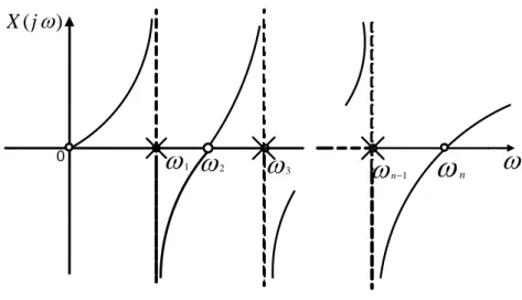
, ) )...( )( ( ) )...( )( ( ) ( 1 2 2 2 4 2 2 2 2 2 2 2 3 2 2 1 2 1 n n j K j Z (3.7) ) )...( )( ( ) )...( )( ( ) ( 2 2 2 3 2 2 1 2 1 2 2 2 4 2 2 2 2 1 n n j K j Z . (3.8) Out of these four forms listed above we can synthesize various different physically realizable reactance networks. Also it is possible to derive and synthesize susceptance functions having the same forms as physically realizable networks. These equations are formed by F. M. Foster. He showed the poles and zeros by 1,2,...n1,n. As K is a positive real constant and1 2 3...n1n, mutual separation of the poles and zeros are accountes.
The reactance plot of the function we have seen in (3.5) which has a zero at 0 and poles at ω = ∞, will have such a form:
14
Figure 3.1 Reactance plot for Eq. (3.5) Such a network will pretend like an inductor at low and high frequencies.
The reactance variation of the function we have seen in (3.6), which has zeros at 0and at ω = ∞, will have a frequency similar to the figure above, except that the reactance will approach zero when ω approaches to infinity. Such a network will pretend like an inductor at low frequencies and like a capacitor at high frequencies.
Similarly, reactance variation of the driving-point function we have seen in (3.7), which has poles at 0 and at ω = ∞, will have such a form:
Such a network will pretend like a capacitor at low frequencies and like an inductor at high frequencies.
The reactance variation of the function we have seen in (3.8), which has a pole at 0and a zero at ω = ∞, will have a frequency similar to the figure above, except that the reactance will approach zero when ω approaches to infinity. Such a network will pretend like capacitors at low and high frequencies.
0
1
2
3
n1
n
) (j
X 0
1
2
1 n
n
) (j
X
315
3.1. Foster Canonic Forms
There are several networks that can be synthesized to realize these functions. For instance if the equations shown in (3.5) and (3.6) form a partial-fraction, then the residues k of the conjugate 1
poles1 must have equal magnitudes by using the conjugate poles as denominators. By combining these conjugate poles, the partial-fraction expansion will have such a form:
2 3 2 3 2 1 2 1 0 1 2 2 ) ( j k k k j Z . (3.9)Then, if we substitute p j, and if we replace the constant factors by new constants the equation will be 2 3 2 3 2 1 2 1 0 1( ) p p K p p K p K p Z (3.10)
While the term K0p stands for an inductor of K henrys, the 20
nd
, 3rd, 4th, etc. terms will take the
form
2
1 2 0 p p K, same as the impedance of a parallel combination of inductance and capacitance, which was previously indicated in equation:
Series combiniation: Cp LCp C L p Z p p 1 1 ) ( 2 1 , Parallel combination: 1 1 1 ) ( 2 1 LCp Lp L C p Z p p . (3.11)
In the equation above, whether the expansion was derived from (3.5) or (3.6) determines the form last term. If it was derived from the former, then the form of the last term will
be
2
1 2 1 p p K, whereas if it was derived from the latter the form of the last term will be
p Kn
,
representing a capacitor.
As we have just mentioned, the last term of the (3-10) will depend on from which equation it was derived. On the other hand the first term represents an inductance and the remainder of the terms is a series of parallel LC elements. As it is not possible for constant terms to exist, hence a term having the form of Knp could be combined with the first term, the last term have to have the
form of
p Kn
, if it is present.
We can realize (3.5) and (3.6) as LC networks of the form shown below, since (3.10) represents the sum of a series of impedances derived from them.
16
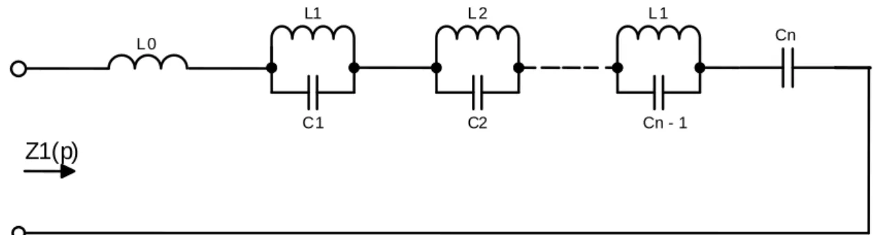
Figure 3.3 First Foster form Considering (3.5), when we expand the function the term
p Kn
will no longer be present,
therefore the last element of the network above, that is the series capacitor, will also no longer be present. It is first element will be an inductor. Considering (3.4),
p Kn
will still be present,
therefore the first element will be an inductor and the last element will be a capacitor.
We can also expand the functions we have seen in the (3.7) and (3.8) in partial fractions by using the conjugate poles as the denominators. Thence, the residues k of the conjugate poles1 1 must have equal magnitudes by using the conjugate poles as denominators. By combining these conjugate poles, the partial-fraction expansion will have such a form:
2 4 2 4 2 2 2 2 0 1 2 2 ) ( j k k k j Z . (3.12)Then, if we substitute p j, and if we replace the constant factors by new constants the equation will be 2 4 2 4 2 2 2 2 0 1( ) p p K p p K p K p Z (3.13)
In the latter equation, while the term
p K0
stands for series capacitor, the 2nd, 3rd, 4th, etc. terms of the function stand for parallel LC combinations, which were previously indicated in (3.10). In the equation above, whether the expansion was derived from (3.7) or (3.8) determines the form last term. If it was derived from (3.7), then the form of the last term will beKnpwhich indicates that a series inductor is present, whereas if it was derived from (3.8) the form of the last term will be
2
1 2 1 p p K. Consequently, (3.13) indicates that the type of networks formed will be same for equations (3.5) and (3.6) and for (3.7) and (3.8).
L1 C1 L2 C2 L1 Cn - 1 L0 Cn Z1(p)
17 We can also use the admittance functions
) ( 1 ) ( 1 2 p Z p
Y to realize the (3.5), (3.6), (3.7) and
(3.8). Similar to the method we use for impedance functions, when we expand the admittance functions in partial-fraction expansions, the result will be the terms of the
form
2
1 2 1 , , p p K p K Kp. If present, the first and/or last terms of the expansion will be of the
form Kp or
p K
, the former denoting a capacitor of K farads and the latter denoting an inductor
of K
1
henrys. The remaining terms will be of the form
2
1 2 1 p p Krepresenting the admittance of a series LC combination. To exemplify, the impedance of a series LC combination shown in equation (3.11) was given as
p C LCp2 1
. Therefore, its admittance will be
1 2
LCp Cp
. As a result,
the impedance of (3.5), (3.6), (3.7) and (3.8) can be realized as admittance functions, so that a second type of network will be formed, which is demonstrated in the figure above.
Figure 3.4 Second Foster form
The equations (3.5), (3.6), (3.7) and (3.8) will determine if a parallel inductor or capacitor will be present as the first or last element of the network.
The networks we have seen in Figures 3.3 and 3.4 are the first two forms of pure reactance networks that were developed by R.M.Foster, therefore sometimes called as the Foster canonic forms. They entail networks that are able to represent any given impedance function through a minimum number of elements. The minimum number of elements that a pure reactance network would have is 2 1 m n
, where n represents the degree of the highest-order terms in the
Ln-1 L0 L2 L1 C1 C2 Cn-1 Cn Y1(p)
18
numerator polynomial and m represents the degree of the highest-order terms in the denominator of the driving-point function.
3.2. Cauer Canonic Forms
We can show the driving-point impedance for a pure LC network as the ratio of two Hurwitz polynomials. As it is unity that the highest-order terms of the numerator and denominator polynomials differ in degree, we can presume that the numerator is of nth order and the denominator is of (n1) order. Accordingly we may write the impedance as such:
5 5 3 3 1 4 4 2 2 1( ) n n n n n n n n n n p a p a p p a p a p K p Z . (3.14)
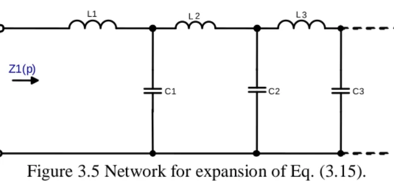
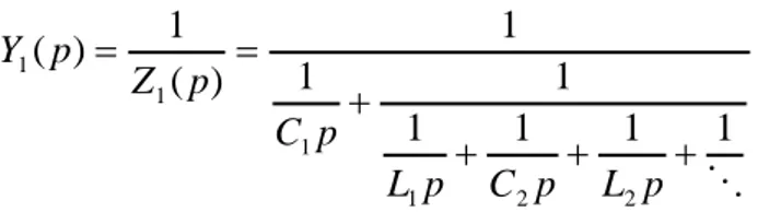
We may expand such a function through a process of long division and inversion to produce a continued-fraction expansion. Such a continued-fraction expansion is likely to have a form shown above: p C p L p C p L p Z 2 2 1 1 1 1 1 1 ) ( . (3.15)
In the expansion, we have substituted the multiplying constants by new constants, namely, ,
2 2 1 1,C ,L ,C
L etc. Accordingly, the above equation may suggest a third form of network, which is shown below (Figure 3.5). The last term of the continued-fraction expansion being an inductor or a capacitor determines the way in which the network will be ceased.
We can also invert the impedance function of (3.14) in order to give an admittance of
) ( 1 ) ( 1 1 p Z p
Y . Hence, we may also expand the admittance to produce a continued fraction
which can have such a form:
C1 C2 C3
Z1(p)
1
L L2 L3
19 1 1 1 1 1 1 1 ) ( 1 ) ( 2 2 1 1 1 1 p L p C p L p C p Z p Y . (3.16) Then, we have substituted the multiplying constants by new constants, namely, L1,C1,L2,C2,etc. again. Accordingly, the above equation may suggest a fourth form of network, which is shown below (Figure 3.6). The last term of the continued-fraction expansion being an inductor or a capacitor determines the way in which the network will be ceased.
We may also presume that in the driving-point impedance of equation (3.14), the denominator is of nth order and the numerator is of (n1) order, hence derive the networks that are shown in Figures 3.5 and 3.6. In such a situation the expansion of
) ( 1 ) ( 1 1 p Z p
Y will yield a network in
the form of Figure 3.5 and the expansion of Z1(p) will yield a network in the form of Figure 3-6. Also, another two canonic forms of reactance functions will be produced out of these networks. For example, suppose we have a continued-fraction expansion that we use for testing a Hurwitz polynomial. We separate the polynomial into E(p) and O(p), E(p) standing for the even powers of s and O(p) standing for the odd powers of s. In order to run the test, we need to develop expansions of either ) ( ) ( ) ( p O p E p R or ) ( ) ( ) ( p E p O p
R till we determine each coefficients. The
coefficients must be positive real numbers; hence the expansion must produce n of them for to let the nth order polynomial be positive real.
Suppose that we choose n as an even number. Then, E(p) will be an even-ordered polynomial of order n, and O(p) will be an even-ordered polynomial of order(n1), for a reactance function. The ratio ) ( ) ( ) ( p E p O p
R will have the form that of equation (3.14). If it is positive real, then there
could be only n terms in its continued-fraction expansion. When we choose n as an odd number, then O(p) will be an odd-ordered polynomial of order n, and E(p)will be an odd-ordered
C3 C2 C1 L3 L1 L2 Z1(p)
20
polynomial of order(n1), for a reactance function. This time the expansion of
) ( ) ( ) ( p E p O p R
must have only n terms. As a result, as it is unity that the highest-order terms of the numerator and denominator of a reactance function would differ, the continued- fraction expansion of these functions will always produce n terms.
The elements of a canonic reactance network will be
2 ) 1
(nm . Here, n stands for the degree
of the highest-order terms in the numerator and m stands for the degree of the highest-order terms in the denominator of the reactance function. The canonic form will have n elements for a numerator with a degree of n and denominator with a degree of nm1. Accordingly, the network that represents the continued-fraction expansion of the reactance function must also be canonic. When the highest-order term of the denominator is greater than the highest-order term of the numerator by unity, the case will be quite the similar.
The figure belows reprents a summary of the canonic Foster and Caurer forms.
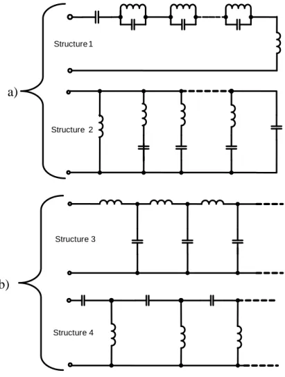
Figure 3.7 Canonic Structures of LC Ladder Networks, a) Foster‟s forms b) Cauer‟s forms
Structure 2 a) Structure 3 b) Structure 4 Structure 1
21
CHAPTER 4
PROPOSED SYNTHESIS PROCEDURES 4.1. Synthesis via Scattering Transfer Matrix Factorization
Decomposition of a lossless two-port network is a classical problem which has been formulated in the literature in many different ways. The conventional approach is to start from a given driving-point function (impedance or reectance) and extract elementary sections, depending on the nature of the transmission zeros being extracted. In this approach, the extraction mechanics and the computation of the remaining impedance or reflectance functions can be quite involved and usually require intensive computational operations. An alternative way of accomplishing the canonic decomposition of lossless two-ports in cascade involves factoring the chain matrix or the scattering transfer matrix. It has long been recognized that the transfer matrix constitutes a better tool, mainly because of the simple representation in terms of only three canonical polynomials [5]. The factorization of the transfer matrix of a lossless two-port into a product of two simpler transfer matrices has been treated rigorously by Fettweis [6,7]. The problem is reduced to the solution of a set of linear equations introducing a mathematically well formulated alternative for the conventional cascade synthesis problem. The methods works directly on the canonic polynomial description of two-ports and involves algebraic decomposition of a given polynomial set, which describes the transfer matrix of a lossless two-port into subsets of polynomials of the same type.
As it is well known, canonic forms of the scattering matrix S and the scattering transfer matrix T of a lossless two-port N, referred to a real terminating resistances are defined as
) ( ) ( ) ( ) ( ) ( 1 , ) ( ) ( ) ( ) ( ) ( 1 ) ( p g p h p h p g p f T p h p f p f p h p g p S (4.1)
where g( p) is a strictly Hurwitz polynomial of degree n , and h( p) and f( p) are real polynomials of degreesn satisfying the paraunitary relation
) ( ) ( ) ( ) ( ) ( ) (p g p h p h p f p f p g (4.2)
22
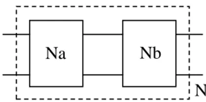
Figure 4.1 Decomposition of a lossless two-port
The problem is to decompose the lossless reciprocal two-port N into two cascade connected lossless two-ports Na and N which are also reciprocal (Fig 4.1). This amounts to factoring the b
transfer matrix T into a product of two transfer matrices [8],
) ( ) ( ) (p T p T p T a b (4.3) where . ) ( ) ( ) ( ) ( ) ( 1 ) ( , ) ( ) ( ) ( ) ( ) ( 1 ) ( p g p h p h p g p f p T p g p h p h p g p f p T b b b b b b b b a a a a a a a a (4.4)
The polynomial sets
ga(p),ha(p),fa(p)
and
gb(p),hb(p),fb(p)
have the same properties as
g(p),h(p),f(p)
and in particular must satify paraunitary relations similar to (4-3), i.e.,) ( ) ( ) ( ) ( ) ( ) (p g p h p h p f p f p ga a a a a a , (4.5) ) ( ) ( ) ( ) ( ) ( ) (p g p h p h p f p f p gb b b b b b . (4.6)
Equation (4) implies the following: ) ( ) ( ) ( ) ( ) (p g p g p h p h p g a b a a b , (4.7) ) ( ) ( ) ( ) ( ) (p h p g p g p h p h a b a a b , (4.8) ) ( ) ( ) (p f p f p f a b , (4.9) b a . (4.10) Under the use of these equalities, if one writes Tb(p)Ta1(p)T(p), three equations can be obtained as ) ( ) ( ) ( ) ( ) ( ) ( ) ( p f p f p h p g p g p h p h a a a a a b , (4.11) Na Nb N
23 ) ( ) ( ) ( ) ( ) ( ) ( ) ( p f p f p h p h p g p g p g a a a a b , (4.12) ) ( ) ( ) ( p f p f p f a b , (4.13) a b . (4.14)
So if the scattering transfer matrix describing the network is given, the following synthesis algorithm can be proposed: The component type and its value is determined via the given scattering transfer matrix. Then the polynomials of the extracted component are formed, and by using Tb(p) Ta1(p)T(p)
expression, the polynomials of the remaining network are obtained. This process is repeated until the termination resistance is reached.
4.2. Low-Pass Case
The scattering transfer matrix of the low-pass network is given as
) ( ) ( ) ( ) ( ) ( 1 ) ( p g p h p h p g p f p T (4.15)
where the polynomials g( p), h( p) and f( p) can be written as follows
n np g p g p g g p g 2 2 1 0 ) ( , (4.16) n np h p h p h h p h 2 2 1 0 ) ( , (4.17) 1 ) (p f . (4.18) Component value of the element that will be extracted can be calculated as
1 1 n n n n h g h g CV (4.19) where n n g h
, and if 1, the component is a series inductor, if 1, the component is a
paralel capacitor.
Then the polynomials (hc(p),gc(p),fc(p)) and their paraconjugates (hc(p),gc(p),fc(p))
of the extracted series inductor or paralel capacitor can be calculated as p CV hc p hc p hc 2 ) ( 1 0 , hc p hc p hc CV p 2 ) ( 1 0 , (4.20) 1 2 ) (p gc1pgc0 CV p gc , 1 2 2 ) (p gc1pgc0 CV p gc , (4.21)
24 1
) (p
fc , fc(p)1, C 1 if the component is a series inductor and C 1 if the
component is a paralel capacitor.
By using these polynomials and the constant C, scattering transfer matrix of the component can be formed as ) ( ) ( ) ( ) ( ) ( 1 ) ( p g p h p h p g p f p T c c c c c c c c . (4.22)
Then scattering transfer matrix of the remaining network can be calculated as
) ( ) ( ) ( ) ( ) ( 1 ) ( ) ( ) ( 1 p g p h p h p g p f p T p T p T R R R R R R R c R . (4.23)
The second component can be extracted by using the polynomials of the remaining network, ) ( ), ( ), (p g p f p
hR R R and the constant R.
The extraction of the components proceeds in a similar fashion until the final termination resistance is reached.
4.2.1. Low-Pass Case Example
The scattering transfer matrix of the low-pass network is given as
) ( ) ( ) ( ) ( ) ( 1 ) ( p g p h p h p g p f p T
where the polynomials g( p), h( p), f( p) and the constant are given as 4 3 2 60 5 14 ) (p p p p p h , 4 3 2 60 35 24 7 1 ) (p p p p p g , 1 ) (p f , 1. Since 1, the first component is a series inductor, and the value of the inductor is
3 ) 5 ( 1 35 60 1 60 3 3 4 4 h g h g CV .
The polynomials of the component can be written as p p p CV h p h p hc c c 2 3 2 3 1 2 ) ( 1 0 , p p p CV h p h p hc c c 2 3 2 3 1 2 ) ( 1 0 , 1 2 3 1 2 ) (p g 1pg 0 CV p p gc c c ,
25 1 2 3 1 2 ) (p g 1pg 0 CV p p gc c c . 1 ) (p fC and fC(p)1.
Then the scattering transfer matrix of the remaining network is
) ( ) ( ) ( ) ( ) ( 1 ) ( ) ( ) ( 1 p g p h p h p g p f p T p T p T R R R R R R R c R where p p p p h p p p p hR R 2 1 5 20 ) ( , 2 1 5 20 ) ( 3 2 3 2 , p p p p g p p p p gR R 2 11 15 20 ) ( , 2 11 15 20 ) ( 3 2 3 2 , 1 ) (p fR , fR(p)1.
Then calculate the new constant () via the polynomials of the remaining network obtained above to decide the type of the second component as follows;
1 20 20 3 3 g h
. Since 1, the second component is a paralel capacitor. The value of
the paralel capacitor is
2 5 1 15 ) 20 ( 1 20 2 2 3 3 h g h g CV .
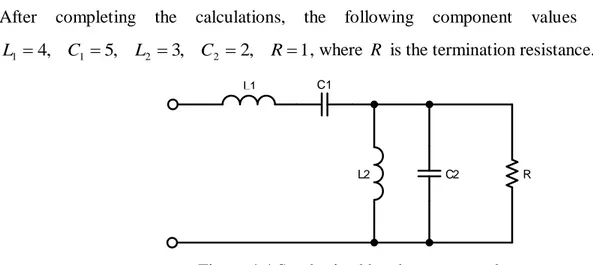
After completing the calculations, the following component values are obtained, 1 , 4 , 5 , 2 , 3 1 2 2 1 C L C R
L , where R is the termination resistance.
R
C 1 C 2
L 2 L 1
26
4.3. High-Pass Case
The scattering transfer matrix of the high-pass network is given as
) ( ) ( ) ( ) ( ) ( 1 ) ( p g p h p h p g p f p T (4.24)
where the polynomials g( p), h( p) and f( p) can be written as follows
n np g p g p g g p g 2 2 1 0 ) ( , (4.25) n np h p h p h h p h 2 2 1 0 ) ( , (4.26) n p p f( ) . (4.27) Component value of the first element that will be extracted can be calculated as
0 0 1 1 h g h g CV (4.28) where 0 0 g h
, and if 1, the first component is a series capacitor, if 1, the first
component is a paralel inductor.
Then the polynomials (hc(p),gc(p),fc(p)) and their paraconjugates (hc(p),gc(p),fc(p))
of the extracted series capacitor or parallel inductor can be calculated as
CV h p h p hC C C 2 ) ( 1 0 , CV h p h p hC C C 2 ) ( 1 0 (4.29) CV p g p g p gC C C 2 1 ) ( 1 0 , CV p g p g p gC C C 2 1 ) ( 1 0 (4.30) p p
fc( ) , fc(p)p, C 1 if the component is a series capacitor and C 1 if the component is a paralel inductor.
By using these polynomials and the constant C, scattering transfer matrix of the component can
be formed as ) ( ) ( ) ( ) ( ) ( 1 ) ( p g p h p h p g p f p T c c c c c c c c . (4.31)
Then scattering transfer matrix of the remaining network can be calculated as
) ( ) ( ) ( ) ( ) ( 1 ) ( ) ( ) ( 1 p g p h p h p g p f p T p T p T R R R R R R R c R . (4.32)
The second component can be extracted by using the polynomials of the remaining network, ) ( ), ( ), (p g p f p
27
The extraction of the components proceeds in a similar fashion until the final termination resistance is reached.
4.3.1. High-Pass Case Example
The scattering transfer matrix of the high-pass network is given as
) ( ) ( ) ( ) ( ) ( 1 ) ( p g p h p h p g p f p T
where the polynomials g( p), h( p), f( p) and the constant are given as 2 1667 . 0 0556 . 0 0139 . 0 ) (p p p h , 3 2 5 . 0 1111 . 0 0139 . 0 ) (p p p p g , 3 ) (p p f , 1. Since 1, the first component is a series capacitor, and the value of the capacitor is
6 0139 . 0 0139 . 0 0556 . 0 1111 . 0 0 0 1 1 h g h g CV .
The polynomials of the component can be written as
12 1 6 2 1 2 ) ( 1 0 CV h p h p hC C C 12 1 6 2 1 2 ) ( 1 0 CV h p h p hC C C , 12 1 6 2 1 2 1 ) ( 1 0 p p CV p g p g p gC C C , 12 1 6 2 1 2 1 ) ( 1 0 p p CV p g p g p gC C C , p p fC( ) and fC(p)p. Then the scattering transfer matrix of the remaining network is
) ( ) ( ) ( ) ( ) ( 1 ) ( ) ( ) ( 1 p g p h p h p g p f p T p T p T R R R R R R R c R where p p h p p hR( )0.08330.0833 , R( )0.08330.0833 , 2 2 4167 . 0 0833 . 0 ) ( , 4167 . 0 0833 . 0 ) (p p p g p p p gR R , 2 ) (p p fR , 2 ) ( p p fR .
28
Then calculate the new constant () via the polynomials of the remaining network obtained above to decide the type of the second component as follows;
1 0833 . 0 0833 . 0 0 0 g h
. Since 1, the second component is a paralel inductor. The value
of the paralel capacitor is
3 0833 . 0 0833 . 0 0833 . 0 4167 . 0 0 0 1 1 h g h g CV .
Figure 4.3 Synthsizes high-pass network
After completing the calculations, the following component values are obtained, 1 , 2 , 3 , 6 1 2 1 L C R
C , where R is the termination resistance.
4.4. Band-Pass Case
The scattering transfer matrix of the band-pass network is given as
) ( ) ( ) ( ) ( ) ( 1 ) ( p g p h p h p g p f p T (4.33)
where the polynomials g( p), h( p) and f( p) can be written as follows
n np g p g p g g p g 2 2 1 0 ) ( , (4.34) n np h p h p h h p h 2 2 1 0 ) ( , (4.35) 2 / ) (p pn f . (4.36)
The constant can be calculated as
0 0 g h
. If 1, the block that will be extracted is series
connected series-LC section, and the component values of this series-LC section can be calculated via the following equations
1 1 n n n n h g h g L and 0 0 1 1 h g h g C . (4.37)
Then the polynomials (hc(p),gc(p),fc(p)) and their paraconjugates (hc(p),gc(p),fc(p))
of the extracted series inductor and series capacitor can be calculated as;
C1 C2
29 For series inductor:
p L hc p hc p hc 2 ) ( 1 0 , hc p hc p hc L p 2 ) ( 1 0 , (4.38) 1 2 ) (p gc1 pgc0 L p gc , 1 2 2 ) (p gc1pgc0 L p gc , (4.39) 1 ) (p fc , fc(p)1, C 1. (4.40) For series capacitor:
C h p h p hC C C 2 ) ( 1 0 , C h p h p hC C C 2 ) ( 1 0 (4.41) C p g p g p gC C C 2 1 ) ( 1 0 , C p g p g p gC C C 2 1 ) ( 1 0 (4.42) p p fc( ) , fc(p)p, C 1. (4.43) By using these polynomials belong to the series inductor and the constant C, scattering transfer matrix of the series inductor can be formed as
) ( ) ( ) ( ) ( ) ( 1 ) ( p g p h p h p g p f p T c c c c c c c c . (4.44)
Then scattering transfer matrix of the remaining network can be calculated as
) ( ) ( ) ( ) ( ) ( 1 ) ( ) ( ) ( 1 p g p h p h p g p f p T p T p T R R R R R R R c R . (4.45)
Then by using these polynomials belong to the series capacitor and the constant C, scattering transfer matrix of the series capacitor can be formed as
) ( ) ( ) ( ) ( ) ( 1 ) ( p g p h p h p g p f p T c c c c c c c c . (4.46)
Then scattering transfer matrix of the remaining network can be calculated as
) ( ) ( ) ( ) ( ) ( 1 ) ( ) ( ) ( 1 p g p h p h p g p f p T p T p T R R R R R R R c R . (4.47)
If 1, the block that will be extracted is parallel connected parallel-LC section, and the component values of this parallel-LC section can be calculated via the following equations
0 0 1 1 h g h g L and 1 1 n n n n h g h g C . (4.48)
Then the polynomials (hc(p),gc(p),fc(p)) and their paraconjugates (hc(p),gc(p),fc(p))
![Figure 2.1 General two-port network [1].](https://thumb-eu.123doks.com/thumbv2/9libnet/4342969.71987/13.892.181.637.591.766/figure-general-two-port-network.webp)