Computation of two-variable mixed element network functions

(1)

KADIR HAS UNIVERSITY

GRADUATE SCHOOL OF SCIENCE AND ENGINEERING

COMPUTATION OF TWO-VARIABLE MIXED ELEMENT NETWORK

FUNCTIONS

NAUMAN TABASSUM

(2)

(3)

Na uman T ab assum (M.S) The sis June 20 18 S tudent’ s F ull Na me P h.D. (or M.S . or M.A .) The sis 20 11

(4)

COMPUTATION OF TWO-VARIABLE MIXED ELEMENT NETWORK

FUNCTIONS

NAUMAN TABASSUM

Submitted to the Graduate School of Engineering In partial fulfillment of the requirements for the degree of

Master of Science In

Electronics Engineering

KADIR HAS UNIVERSITY ISTANBUL, JUNE 2018

(5)

(6)

(7)

ii

List of Figures

Figure 1.1 Lossless Two-port Darlington equivalent Network (Darlington, 1939). ... 3

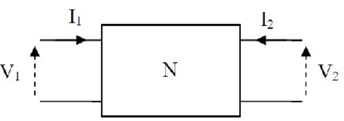
Figure 2.1 General two-port network (four-terminal network). ... 6

Figure 2.2 Doubly terminated two-port network (Medely, 1993) ... 7

Figure 2.3 Representation of transmission line unit elements and their counterparts in Richards transformation (ŞENGÜL, 2006). ... 19

Figure 2.4 Application of Richards theorem. ... 20

Figure 3.1 Simple Lumped Section. ... 24

Figure 3.2 Simple Distributed Section. ... 27

Figure 3.3 a) Cascaded Distributed Design and Lossless Lumped Ladder. b) Cascaded Decomposition. c)Cascade of Simple Lumped and Distributed Section. ... 34

Figure 3.4 Low-pass Ladder with Unit Elements. ... 42

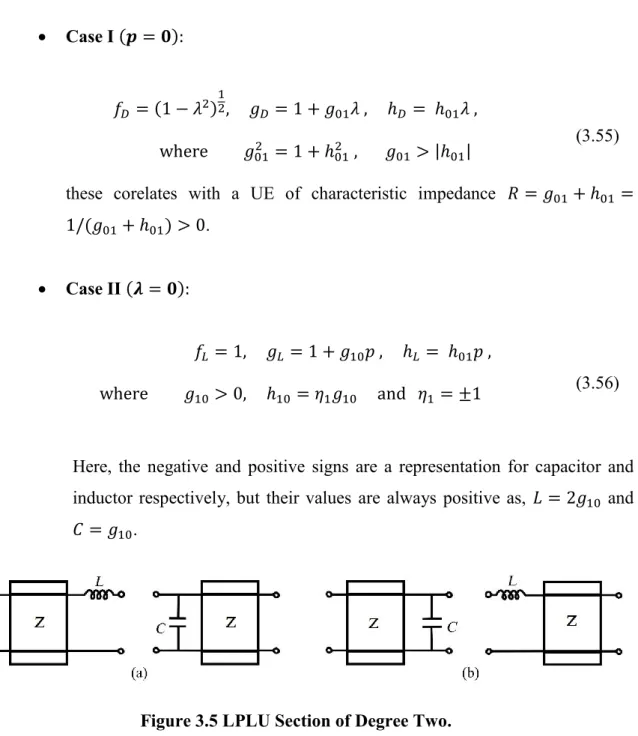
Figure 3.5 LPLU Section of Degree Two. ... 46

Figure 3.6 LPLU Section of Degree Three. ... 48

Figure 3.7 LPLU Section of Degree Four. ... 52

Figure 3.8 LPLU Section of Degree Five. ... 56

Figure 3.9 Higher Order LPLUs as Cascades of Elementary LPLU Section. ... 60

Figure 4.1 Physical Realization of LPLU Section of Degree Five (𝒏𝒑 = 𝟑, 𝒏𝝀 = 𝟐 ). ... 64

Figure 4.2 Example N0.1 Physical Realization of LPLU Section of Degree Five (𝒏𝒑 = 𝟐, 𝒏𝝀 = 𝟑 ). ... 69

Figure 4.3 Example No.2 Physical Realization of LPLU Section of Degree Five (𝒏𝒑 = 𝟐, 𝒏𝝀 = 𝟑 ). ... 71

(10)

v

COMPUTATION OF TWO-VARIABLE MIXED ELEMENT NETWORK FUNCTIONS

Abstract

In this dissertation , the algorithm known as “Standard Decomposition Technique (SDT)” is used together with Belevitch’s canonic representation of scattering polynomial for two-port networks operate on high frequency, to find the analytical solutions for “Fundamental equation

set (FES)”. This FES is extracted by using Belevitch canonic polynomials “ 𝑔(𝑝, 𝜆), ℎ(𝑝, 𝜆)

and 𝑓(𝑝, 𝜆)” used for the description of mixed lumped and distributed lossless two-port cascaded networks in two variables of degree five and the obtained solutions are further used to synthesis the realizable networks. The solution to the problem is also classified into two cases, first case is discussed for three lumped and two distributed (𝑛𝑝 = 3, 𝑛𝜆 = 2 ) and the second is for three distributed and two lumped important (𝑛_𝑝 = 2, 𝑛𝜆 = 3 ) the solution for both these cases are expressed separately with conclusive examples.

Keywords: Standard Decomposition Technique (SDT), Belevitch’s canonic representation,

scattering polynomials, Two-port networks, Fundamental equation set (FES), Mixed lumped and distributed lossless networks, Cascaded networks in two variables, Networks of degree five.

(11)

vi

İKİ DEĞİŞKENLİ KARIŞIK ELEMANLI DEVRE FONKSİYONLARININ HESABI

Özet

Bu tezde, Standart Ayrıştırma Tekniği (SDT) olarak bilinen algoritma, yüksek frekansta çalışan iki portlu ağlar için Belevitch'in saçılma polinomunun kanonik gösterimi ile birlikte, Temel Denklem Seti (FES) için analitik çözümler bulmak amacıyla kullanılmıştır. Bu denklem seti, Belevitch’in iki değişkenli karışık toplu ve dağıtılmış kayıpsız iki portlu kaskad ağların tanımı için kullanılan g (p, λ), h (p, λ) ve f (p, λ) kanonik polinomlarından elde edilmiş ve elde edilen sonuçlar daha sonra gerçeklenebilir devrelerin sentezinde kullanılmıştır. Problem üç toplu ve iki dağıtılmış (𝑛𝑝 = 3, 𝑛𝜆 = 2 ) ile iki toplu ve üç dağıtılmış (𝑛𝑝 = 2, 𝑛𝜆 = 3 ) eleman olacak şekilde iki ayrı durum için ele alınmış ve çözüm her bir durum için ayrı ayrı verilmiştir.

Anahtar Kelimeler: Standart Ayrıştırma Tekniği (SDT), Belevitch'in kanonik gösterimi,

Saçılma polinomları, İki portlu ağlar, Temel denklem seti (FES), Karışık lumped ve dağıtık kayıpsız ağlar, İki değişkenli basamaklı ağlar, Beşinci dereceden ağlar.

(12)

vii

Acknowledgements

In the name of Allah, the most Gracious, the most Merciful and the most Beneficent. I am thankful to Almighty Allah for giving me strength and blessed me with all kind of needs to complete my thesis. I would love to offer my heartiest praises to the Prophet Muhammad (ﷺ), the Mightiest and final Prophet of Almighty Allah, has been sent as the best of teachers to humankind, to teach humanity and to live a purposeful life.

Special appreciation goes to Dr. Atilla ÖZMEN, who is not just my thesis advisor but also a nice and kind human being in all aspects of life. I am thankful, from the depth of my heart for his through supervision, continuous support and precious pieces of advice, without his efforts, this dissertation would not even be anywhere near to possible. I believe he put his best to make my efforts into a success. It is only because of his insight, enthusiasm and continuous encouragement which helped me to complete this task. I would also like to thank and appreciate Dr. Metin ŞENGÜL, co-advisor to my work, for the guidelines and ideas. I found him one of the best in the field, I have learned a lot from his work and his research was a great help to complete my thesis. This was an honor and great learning experience to work with both of these personalities.

I express my deepest gratitude to all the faculty member of Department of Electrical and Electronics Engineering and Graduate School of Science and Engineering, especially Dr. Ayşe Hümeyra BİLGE, Dr. Funda SAMANLIOĞLU, DR. Hakan Ali ÇIRPAN, Dr. Arif Selçuk ÖĞRENCİ and Dr. Serhat ERKÜÇÜK.

I would also like to thank my parents, Mr. Ghulam Farid and Mrs. Shafqat Bibi, because without them I am nothing, both of them are very important part of my life and a driving force for me to find positive ways for existence and to achieve goals. They are the reason behind all of my success and learnings. I am grateful for all of their support and prays that made me finish this degree with success. My parents are my mantors. I would like to thank my brothers and sisters Mr. Adnan Farid, Miss. Ayesha Farid, Miss. Aqsa Farid, Mr. Muhammad Usman Farid, and Mr. Muhammad Ateeq-ur- Rehman for having belief in me and showing their presence at the time of need and making my family the best family and keeping my home a sweet home.

(13)

viii

Finally, I would like to thank some of my Turkish friends, Mr. Hakan TURAN, Miss. Zozan KARAKAŞ, my brother Mr.Yasin KOÇ and a great family of Mr. Serdar CELEBCI his wife Miss Perveen and their small daughter Maya for their great love and hospitality. I would like to thank my friends especially Mr. Waqas Khan Abbasi, Mr. Abdul Mohemine, Mr. Mohsin Kiani and Miss. Zoya Javaid for supporting me and giving me the best of advice. There are lots of name of friends and relative I want to count but cannot point them all, so compositely I am thankful to all for being a beautiful part of my life.

I am completing the segment of the novel with this prayer.

ِّ بَر

ِّ نا َس لِّ رن مًِّةَدرقُعِّرلُلرحاَوِّي ررمَأِّ لِِّ ر سَّيَوِّي ررد َصِّ لِِّ رحَ رشْا

ِّ لِ روَقِّاوُهَقرفَي

(ن آرقلا)

ِّ

O my Lord! Open for me my chest (grant me self-confidence, contentment, and boldness); Ease my task for me; And remove the impediment from my speech, so they may understand what I say (Al-Quran)

(14)

ix

Dedication

ًنا َسْح

ا انْي َ الِاَوْل ابَِو

_ِ

(ن آرقلا(

And treat you parents with kindness (Al-Quran)

(15)

(16)

1 INTRODUCTION

1.1 Overview

In the field of communication systems design and development, one of the most crucial problems is to design a coupling circuit model, that work over a broadest attainable frequency band to achieve optimum performance. A coupling circuit is used to match one device to another, also known as impedance matching network or equalizer network. Characteristically, the problem here is to design an impedance matching network, to convert a provided impedance to a particular one, the phenomenon usually referred to as equalization or impedance matching. The problem of designing, matching networks was considered seriously in literature for several decades. The development of millimeter-wave and microwave integrated circuit technology motivated new ventures in the design and development of wideband communication systems and also stimulated a renewed interest in broadband matching.

High-frequency telecommunication systems such as satellites, antennas, amplifiers, filter and high-frequency transistors contain front-end, inter-stage, and back-end blocks and these blocks can be distinguished and classified by their measured data. For these type of high-frequency systems, to control the power flow between above-described stages, filters and equalizer circuits are designed by using recognized analytical and semi-analytical techniques. Modeling of numerically explained components is mandatory, either by practicable circuit functions or components. From this discussion, aim is to develop ability to model numerically define device by mean of lossless components by using recent analytic design methods (ŞENGÜL, 2006).

1.2 Literature Review

It is contemplated that the broadband matching theory is originated after the development of restricted load impedance gain-bandwidth theory and restricted load impedance is composed of a parallel combination of a resistor and a capacitor (Bode, 1945). After more developments, a generalized gain-bandwidth theory is presented for any random load impedance (Fano, 1950) (Youla, 1964). Circuit modeling is critically important to design broadband matching circuits

(17)

2

(Chen, 1988). The requirement is to develop an optimum lossless two-port matching network (Carlin & Amstutz, 1981) that is able to transfer maximum power between load and source at broadest possible frequency band (Aksen, 1994). Here, source and load can be represented by numerical data and can also be considered as complex one port networks (ŞENGÜL, 2006) (Yarman, 1982). To implement the Analytical Gain-Band Width Theory (Carlin, 1977) (Belevitch, 1968) it is necessary to understand basic of complex one port networks. Later on, to encounter the broadband matching problems many other researchers had published extended works with better elaboration. While working with complex practical application and designing complicated matching circuits, the current broadband matching theory faces serious problems. Therefore, plenty of literature is available that focused on finding more practical ways to design matching networks.

Precious work is available in the literature about data modeling (Smilen, 1964) (Baum, 1948) is available but semi-analytic computer-aided and numerical techniques are practiced because of difficulties and presence of inaccuracy in existing methods of modeling the matching problems (Kody & Stoer, 1972) (Kotiveeriah, 1972). Carlin (Carlin, 1977) and Yarman (Carlin & Yarman, 1983) proposed Real Frequency Technique (RFT), further advancements are made by several researchers to encounter the difficulties of modeling the matching problems. These latest and efficient and accurate modeling and matching with help of analytic methods are still unable to answer all fundamental problems for researchers (Yarman, 1982) (Yarman, 1982) (Beccari, 1984) (Yarman & Aksen, 1992). To full the industrial requirements like microwave amplifier design problems and equalizer circuit design problems several computer programs have been developed (Hatley, 1967). Although these circuit design computer programs are very helpful for several practical problems but still insufficient to encounter all kinds of complicated design problem, as their working principle is Brute Force method (Yarman & Fettweis, 1990) (Fettweis & Pandel, 1987) (Yarman, 1985) (Carlin & Civalleri, 1985).

It is a normal practice to define the load is by reflection parameters calculated in the desired frequency bandwidth or by amplitude and phase or real and imaginary pairs. While modeling such types of numerical data, the circuit functions realizability conditions and constraints must be considered. Here, a numerical defined physical device as a lossless two-port network (Darlington equivalent) (Darlington, 1939).

(18)

3

Figure 1.1 Lossless Two-port Darlington equivalent Network (Darlington, 1939).

In literature, to model, the impedance data two most widely used methods are:

1. Select a network topology and designate the best appropriate values of components. 2. Determination of impedance or reflection function which is suitable for the data and

synthesizes the function to obtain the model.

In the first method, an optimization tool is applied, after choosing the network topology, to define the suitable values to component. Although this is a very easy and uncomplicated method, it carries some difficulties: The process of optimization is highly nonlinear with respect to the values of component, can achieve a local minimum or can diverge from it. The satisfactory result can be achieved after the optimization process, by a proper and careful choice of initial values and it is a very hard task to find suitable initial values (Yarman, 1991). There is an additional obstacle, there is no explicit answer to, what is the suitable network topology for the provided data? Hence, the modeler will try several network topologies to select the best suitable or the problem will be unsolved.

Several data modeling methods are proposed to model the provided impedance or reflection data. In the easiest one, rational functions are used to depict impedance data and by using interpolation, to estimate the coefficients of the function. A similar rational function 𝑍(𝑝) is given in 1.1; 𝑍(𝑝) =∑ 𝛼𝑗𝑝 𝑗 𝑛−1 𝑗=0 ∑𝑛−1𝑗=0 𝛽𝑗𝑝𝑗 𝑗 = 0,1, … … , (𝑛 − 1) (1.1)

(19)

4

where, complex frequency variable 𝑝 = 𝜎 + 𝑖𝜔 and 𝛼𝑗 and 𝛽𝑗 are positive real coefficients. But, positive real function cannot be obtained at the end of this technique. Two other modeling tools are proposed, and these methods are based on working with scattering parameters or input impedance of the device. The first method, named as Immittance Approach, impedance or admittance values are used. Approximation of real part of the input impedance is calculated by using a minimum reactance function, then minimum reactive data is removed after this Foster function is used to model the remaining imaginary data. In the second method, reflection coefficient data is modeled by a bounded function and the method is called Reflection Parameter Approach.

1.3 Thesis Contribution

In the available literature two port networks of degree five consist of mixed lumped and distributed elements, the transfer function and canonic representation are not represented on pure analytical basis. In simple words, there is no analytical solution for LPLU of degree five exist in literature. So, in this study, the objective is to use a modeling method named “Standard

Decomposition Technique” and focus will be on the network consist of the cascade of mixed

lumped and distributed elements of degree five to find analytical solution to the problem.

1.4 Thesis Outline

Chapter 1 of the thesis is an introductory novel to the topic and its brief overview, it is also covering the previous research in the related field with the contribution of this dissertation. Chapter 2 is covering the fundamental concepts of network theory, those are related and helpful for further study. The chapter contains a brief introduction of lossless two-port networks, scattering representation, canonic representation of scattering matrix and mixed, lumped and distributed elements.

In chapter 3 our focus will be on the description of mixed lumped and distributed elements, the issues involving in the fabrication of two-variable network function are also discussed. A semi-analytical technique is presented to elaborate two-port cascaded mixed networks.

In chapter 4 the focus is to find the analytical solutions for LPLU of degree five for some real and realizable values. A two-variable polynomial with degree five is generated LPLU of degree

(20)

5

five, first the discussion is made for three lumped and two distributed (𝑛𝑝 = 3, 𝑛𝜆 = 2 ) and the second will be with three distributed and two lumped important (𝑛𝑝 = 3, 𝑛𝜆 = 2 ) . Chapter 5 is concluding the discussion and developing the remarks, at the end some important Matlab code are given, used to develop the solutions.

(21)

6

2 FUNDAMENTAL PROPERTIES OF LOSSLESS TWO-PORT

NETWORKS

This chapter is dedicated to investigating and discuss the basic ideas related to network theory. A review of basic definition and elementary properties regarding the scattering parameters description of lossless two-port networks has made. Fundamental properties of the network functions related to lossless two-port lumped and distributed networks are elaborated. A brief introduction of mixed lumped and distributed elements network is also discussed.

2.1 Port, Two-Port and n-Port Network

In network theory, a pair of terminals joining an electrical network or a circuit to another external circuit is known as a port and the current entering through one terminal is always equal to the current leaving through the other terminal of a port. These terminals are also called nodes. Circuit components like capacitors, resistors, inductors, transistors etc., may have two or more terminals. The combination of these components in a meaningful manner form networks. Figure 2.1 is representing a two-port lossless network a kind of quadripole network consist of two ports or four terminals also representing the values of voltages and current on each terminal. Generally, mathematical representation obtained from the values of currents and voltages of external terminals are used to determine the source and load response connected to the network.

(22)

7

2.2 Scattering Representation of Two-port Networks

It is a fact that impedance, admittance and transmission parameters are widely used to calculate the terminal response of a two-port lossless network and the also work quite beautifully. Impedance and admittance parameters are determined with respect to infinite or zero loads at the ports although they conclude a useful information about two-port networks. There is no assurance of equally well results for all type two-port networks because of the requirement of infinite or zero loads at the ports. On contrary, scattering parameters are well defined with respect to finite loads and also exist for all kinds of networks. It is well established that scattering parameters are used as a powerful tool to understand the power transfer characteristics of networks like filter and matching networks especially at microwave frequencies, under specific terminations.

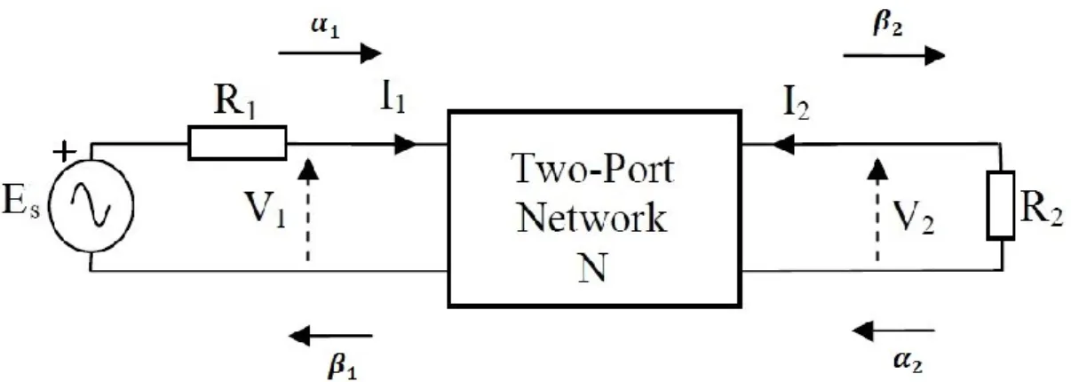
Figure 2.2 Doubly terminated two-port network (Medely, 1993)

Figure 2.2 is referring to a two-port network which is ignited at port 1 by a voltage source 𝐸_𝑠, through impedance R1, and terminated at port 2 by load impedance R2. R1 and R2, can be of any value because they are just reference impedances, although 50Ω is the most commonly used value. Figure 2.2 is explaining the definitions of current 𝐼𝑗, voltage 𝑉𝑗 and impedance 𝑅𝑗 and also, two new parameters 𝛼𝑗 and 𝛽𝑗 can also be defined as (Medely, 1993).

𝛼_𝑗 = 𝑉𝑗+ 𝑅𝑗𝐼𝑗

2√|𝑅𝑒𝑅_𝑗| (2.1)

(23)

8 𝛽_𝑗 = 𝑉𝑗− 𝑅𝑗 ∗_𝐼 𝑗 2√|𝑅𝑒𝑅𝑗| (2.2) by solving 2.1 and 2.2, the results are

𝑉_𝑗 = (𝛼_𝑗+ 𝛽_𝑗)√𝑅𝑒|𝑅𝑗| (2.3) and 𝐼𝑗 = (𝛼_𝑗− 𝛽_𝑗) √𝑅𝑒|𝑅𝑗| (2.4) here 𝑅_𝑗*_{and 𝑅𝑒|𝑅}

𝑗| is the complex conjugate and real part of reference Impedance 𝑅𝑗 respectively. Equations for scattering parameters for two-port in Figure 2.2 can be defined as (Medely, 1993).

𝛽1 = 𝑆11𝛼1 + 𝑆12𝛼2 (2.5)

𝛽₂ = 𝑆₂₁𝛼₁+ 𝑆₂₂𝛼₂ (2.6)

Expression for scattering parameter in matrix form any n-port network is

𝛃 = 𝐒𝛂 (2.7)

The evaluation of coefficients of 2.5 and 2.6 can be estimated by placing 𝛼1 = 0 and 𝛼2 = 0. Now consider the Figure 2.2, the output voltage is −𝐼₂𝑅₂ and substituting this value in 2.1 the result is;

𝛼₂ = −𝑉2𝑅2 + 𝑉2𝑅2 2√|𝑅𝑒𝑅2|

= 0 _(2.8)

If any of the ports is not connected to the source and having reference impedance on termination that specific 𝛼_𝑗 is always zero. Transmission line theory (Medely, 1993) the expression can be written as,

(24)

9

𝑉𝑗 = 𝑣𝑗𝑖+ 𝑣𝑗𝑟 (2.9)

and,

𝐼_𝑗 = 𝑣𝑗𝑖− 𝑣𝑗𝑟

𝑅_𝑗 (2.10)

here the subscripted 𝑖 and 𝑟 are representing the incident component and reflected component of voltage, respectively. Considering 𝑅𝑗to be real and substituting in 2.1

It can be seen in 2.11 that 𝛼_𝑗 is the function of incident voltage and 𝛽_𝑗 is a function of reflected voltage by 2.12. It can also be observed that the squares of 𝛼_𝑗 and 𝛽_𝑗 gives us the dimensions of power. Mathematically; |𝛼𝑗| 2 = |𝑣𝑗𝑖| 2 |𝑅𝑒𝑅𝑗| 𝑎𝑛𝑑 |𝛽𝑗| 2 = |𝑣𝑗𝑟| 2 |𝑅𝑒𝑅𝑗| (2.13)

So, 𝛼𝑗 and 𝛽𝑗 are representing incident and reflected waves respectively, also |𝛼𝑗| 2

and |𝛽𝑗| 2

are representing incident and reflected powers respectively. From 2.5 and 2.6, it can be observed that the reflected wave from any port is equal to the submission of modified incident waves from all the ports, this modification is made by S-parameter matrix.

(25)

10

Mathematically, |𝛼_𝑗|2 can be represented by Figure 2.2,

|𝛼1|2 = | 𝑉₁+ 𝑅₁(𝐸𝑠_𝑅− 𝑉1 1 ) 2√𝑅𝑒𝑅1 | 2 = |𝐸𝑠| 4|𝑅𝑒𝑅₁| (2.14)

Form 2.14 it can be observed that |𝛼1|2 is total power available from the source, by subtracting reflected power from total available power, power delivered to the network can be obtained, that is represented as,

|𝛼_𝑗|2− |𝛽_𝑗|2 = 𝛼_𝑗𝛼_𝑗∗− 𝛽_𝑗𝛽_𝑗∗ =(𝑉1+ 𝑅1𝐼1)(𝑉1 ∗_{+ 𝑅} 1∗𝐼1∗) 4|𝑅𝑒𝑅1| −(𝑉1− 𝑅1𝐼1)(𝑉1 ∗_{− 𝑅} 1∗𝐼1∗) 4|𝑅𝑒𝑅1| =2𝑅1(𝑉1𝐼1 ∗_{+ 𝑉} 1∗𝐼1) 4|𝑅𝑒𝑅₁| (2.15) = 𝑅1 |𝑅𝑒𝑅1| 𝑅𝑒(𝑉₁𝐼₁∗) (2.16)

If the source is terminating port 1, then |𝛼𝑗| 2

will be zero and |𝛽𝑗| 2

can be expressed as,

|𝛽2|2 = | 𝑉₂− 𝑅₂∗𝐼₂ 2√𝑅𝑒𝑅2 | 2 = |𝑅𝑒𝑅2||𝐼2|2 (2.17)

where 2.17 is representing the delivered load power.

Coefficients 𝑆_𝑚𝑛 of S-parameter matrix are representing the ratios between reflected and incident waves, is most appropriate depiction of microwave circuits. When a source with available power |𝛼_𝑗|2 is attached to port 𝑗, value of 𝛼 for port 𝑗 and value of 𝛽 for all ports can be calculated.

(26)

11 𝑆_𝑗𝑗 =𝛽𝑗 𝛼_𝑗 = 𝑉𝑗− 𝑅𝑗∗𝐼𝑗 𝑉_𝑗+ 𝑅_𝑗𝐼_𝑗 = Ω𝑖𝑛𝐼𝑗− 𝑅𝑗∗𝐼𝑗 Ω_𝑖𝑛𝐼_𝑗+ 𝑅_𝑗𝐼_𝑗 = Ω𝑖𝑛− 𝑅𝑗∗ Ω_𝑖𝑛+ 𝑅_𝑗 (2.18)

in 2.18, Ω_𝑖𝑛 is representing the input impedance of port 𝑗. The reflection coefficient of port 𝑗 will be 𝜌_𝑖𝑛 and is equal to 𝑆_𝑗𝑗, power loss at port 𝑗 can be given by,

|𝑆_𝑗𝑗|2 = |𝛽𝑗| 2 |𝛼_𝑗|2 =

Reflected power from input port

Availale power at source to port (2.19)

at any other port 𝑘 and 𝑗 ≠ 𝑘 , transducer power gain can be given as,

|𝑆𝑘𝑗| 2 =|𝛽𝑘| 2 |𝛼𝑗| 2 =

Power delivered to the load

Availale power at source to port (2.20)

By the law of conservation of energy, the total incident power at all the ports of a passive network system must be equal to the power dissipated by in the network and power reflected from the network. The dissipated power by the network can be calculated by subtracting the reflected power from incident power as |𝛼_𝑗|2− |𝛽_𝑗|2. The total dissipated power 𝑃_∆ can be given as the summation of the dissipated powers at every port of the network (Medely, 1993).

𝑃∆ = ∑ ( |𝛼𝑗| 2 − |𝛽𝑗| 2 ) = ∑𝑚𝑗=1𝛼𝑗𝛼𝑗∗− ∑𝑚𝑗=1𝛽𝑗𝛽𝑗∗ 𝑚 𝑗=1 (2.21) or, 𝑃∆= [𝛼∗]𝑡𝛼 − [𝛽∗]𝑡𝛽 (2.22)

here [𝛼∗_]𝑡_{and [𝛽}∗_]𝑡_{are representing the transpose of complex conjugate of each element of 𝛼} and 𝛽. By 2.7,

[𝛽∗_]𝑡_{= [𝑆}∗_]𝑡_[𝛼∗_]𝑡 _(2.23)

substituting 2.23 in 2.22,

(27)

12 after simplifying,

𝑃_∆ = [𝛼∗]𝑡_{{𝐼 − [𝑆}∗_]𝑡_𝑆}𝛼 _(2.25)

the term in curly braces of 2.25 determines whether the dissipated power is positive or negative. The definition can be given as (Medely, 1993).

𝑊 = 𝐼 − [𝑆∗]𝑡_𝑆 _(2.26)

The expression in 2.26 is showing the dissipation matrix and if 𝑊 is nonnegative quantity the behavior of network will be passive means the dissipated power is zero or greater than zero. For two-port passive networks,

|𝑆11|2+ |𝑆21|2 ≤ 1 𝑎𝑛𝑑 |𝑆22|2+ |𝑆12|2 ≤ 1 (2.27) For two-ports lossless networks the power dissipation will be zero and the expression in 2.26 will become, 𝐼 = [𝑆∗_]𝜏_𝑆 _(2.28) or in matrix form, [1 0 0 1] = [ 𝑆₁₁∗ 𝑆₂₁∗ 𝑆₁₂∗ 𝑆₂₂∗ ] [ 𝑆11 𝑆12 𝑆₂₁ 𝑆₂₂] (2.29)

and the can also be

𝑆₁₁∗ 𝑆11+ 𝑆21∗ 𝑆21= 1 (2.30) 𝑆₁₁∗ _𝑆 12+ 𝑆21∗ 𝑆22= 0 (2.31) 𝑆₁₂∗ 𝑆₁₁+ 𝑆₂₂∗ 𝑆₂₁= 1 (2.32) 𝑆₁₂∗ _𝑆 12+ 𝑆22∗ 𝑆22= 0 (2.33)

(28)

13

𝑆₁₁∗ 𝑆11= 𝑆22∗ 𝑆22 𝑎𝑛𝑑 𝑆12∗ 𝑆12= 𝑆21∗ 𝑆21 (2.34)

The relations derived earlier are concluding that the magnitudes of reflection coefficients and transmission coefficients are bounded by unity, i.e. |𝑆_𝑘𝑗| ≤ 1 for 𝑝 = 𝑖𝜔.

The discussion earlier can be summarized as following fundamental properties of lossless two-port networks (ŞENGÜL, 2006) (Aksen, 1994).

1. For real 𝑝 the elements of matrix 𝑆 are real and rational. 2. In 𝑅𝑒 𝑝 ≥ 0 the matrix 𝑆 will be analytic.

3. Matrix 𝑆 is paraunitary and satisfies [𝑆∗_]𝜏_{𝑆 for all 𝑝.}

4. The lossless two port system will be reciprocal if matrix 𝑆 is symmetric, i.e. 𝑆12= 𝑆21.

The corresponding impedance and admittance matrices can be easily estimated if the scattering matrix satisfies all the conditions discussed above. The realizability theory based on Darlington approach, in immittance formalism, can be established and expressed by using the driving point functions of a two-port network terminated at the output by a resistance. At this point of discussion, it is relevant to describe the following fundamental properties in correspondence to the driving point impedance and reflectance functions (ŞENGÜL, 2006) (Aksen, 1994).

• The function 𝑆₁(𝑝) will be bounded and real if

1. For all real 𝑝, 𝑆₁(𝑝) is real.

2. In 𝑅𝑒 𝑝 > 0 the matrix 𝑆₁(𝑝) is analytic. 3. |𝑆₁(𝑖𝜔)| ≤ 1 , ∀ 𝜔.

• The relative input impedance 𝑅1(𝑝) of a resistively terminated two-port can be given as,

𝑅₁(𝑝) =1 + 𝑆1(𝑝)

(29)

14

the impedance function 2.35 is positive real function (p.r.f) and satisfying the following properties as well,

1. For all real 𝑝, 𝑅₁(𝑝) is real. 2. for 𝑅𝑒 𝑝 > 0, 𝑅𝑒 𝑅1(𝑝) > 0.

The conclusion can be made for a resistively terminated two-port network that the realizability of driving point functions that, "A rational and positive real impedance function (or also be a bounded real reflection/impedance function) can be achieved as a resistively terminated lossless two-port”.

2.3 Scattering Transfer Representation of Two-Ports

The more appropriate way of dealing with, cascaded two-port networks, is to use the scattering transfer matrix instead of the scattering matrix. Consider 2.5 and 2.6 , rearrange the port variables 𝛼_𝑗 and 𝛽_𝑗, the rersult can be expressed as

𝛽₁ = 𝑇₁₁𝛼₂+ 𝑇₁₂𝛽₂ (2.36)

𝛼2 = 𝑇21𝛼2+ 𝑇22𝛽2 (2.37)

and the matrix representation of 2.36 and 2.37 is,

[𝛽1 𝛼₂] = [ 𝑇₁₁ 𝑇₁₂ 𝑇21 𝑇22] [ 𝛼₂ 𝛽₂] (2.38)

The definition of scattering transfer matrix 𝑇 is explained in 2.38, the members of matrix 𝑆 are related to the members of matrix 𝑇, as follows,

𝑇11= − det 𝑆 𝑆₂₁ , 𝑇21 = − 𝑆₂₂ 𝑆₂₁ , 𝑇12= 𝑆₁₁ 𝑆₂₁ 𝑎𝑛𝑑 𝑇22 = 1 𝑆₂₁ (2.39)

(30)

15

In 2.39 det 𝑆 is representing the determinant of matrix 𝑆, also the elements of scattering transfer matrix are rational functions, the reciprocity condition for two-port in the case of scattering transfer matrix is 𝑆₁₂= 𝑆₂₁that gives to det 𝑇 = 1.

2.4 Canonic Representation of Scattering and Scattering Transfer Matrix

Scattering parameters of a two-port can also be represented in term of compact three canonic polynomials. The Belevitch canonic representation of scattering matrix and scattering transfer matrix can be given as (Belevitch, 1968),

𝑆 = 1 𝑔[ ℎ 𝜎𝑓_∗ 𝑓 −𝜎ℎ_∗] 𝑎𝑛𝑑 𝑇 = 1 𝑓[ 𝜎𝑔_∗ ℎ 𝜎ℎ_∗ 𝑔] (2.40)

where 𝑓∗= 𝑓(−𝑝) is paraconjugate of a real function. The properties of canonic polynomial 𝑓, 𝑔, 𝑎𝑛𝑑 ℎ are given as (Aksen, 1994) (ŞENGÜL, 2006).

• 𝑓 is monic, i.e. its leading coefficient is equal to unity. • 𝑔 is strictly Hurwitz polynomial.

• 𝑓 = 𝑓(𝑝), 𝑔 = 𝑔(𝑝) and ℎ = ℎ(𝑝) are real polynomials in complex frequency domain. • The relation between 𝑓, 𝑔 and ℎ is,

𝑔𝑔∗ = 𝑓𝑓∗+ ℎℎ∗ (2.41)

• 𝜎 is constant and its value is ±1.

If the two-port network is reciprocal, then the polynomial 𝑓 will be either even or odd in the case of even the 𝜎 = +1 and if it is odd then 𝜎 = −1, so as result,

𝜎 =𝑓∗

𝑓 = ±1 (2.42)

(31)

16

𝑔𝑔_∗ = 𝜎𝑓2+ ℎℎ_∗ (2.43)

as 𝑝 = 𝑖𝜔, and from 2.41,

|ℎ| ≤ |𝑔| 𝑎𝑛𝑑 |ℎ| ≤ |𝑓| (2.44)

which in turn imply following degree relations,

deg ℎ ≤ deg 𝑔 𝑎𝑛𝑑 deg ℎ ≤ deg 𝑓 (2.45)

the notation deg stands for degree of the canonic polynomials, the term deg 𝑔 − deg 𝑓 is representing the number of transmission zeros at infinity and the information about the degree of lossless two-port network lies and equal to the degree of polynomial 𝑔.

In the canonic representation, there is a possibility of the presence of common factor of 𝑔, 𝑓 and ℎ at same time. Simply, generally it is not necessary that 𝑔 is least common divider for scattering polynomial 𝑆𝑘𝑗. For example, consider 𝑔 and 𝑓 have a common factor, the transfer factor 𝑆21will be irreducible from 𝑓/𝑔, and the same description will old for other terms of 𝑆. As from the mentioned characteristics, 𝑔 the common divider is strictly Hurwitz polynomial, so any common factor of the canonic polynomials is also necessarily Hurwitz. Moreover from 2.41, a common factor between any two of three polynomials 𝑔, ℎ and 𝑓 must necessarily divide the third polynomial or its paraconjugate.

A brief discussion about transmission zeros will be part, in next lines. The transmission zeros for a two-post lossless network in forward direction are defined by the zeros of 𝑆21(𝑝) and in revers direction by zeros of 𝑆₁₂(𝑝). Hence, the calculation of total transmission zeros can be estimated by the product of irreducible forms of 𝑓/𝑔 and 𝑓/𝑔_∗, by using 2.41 result is

𝑓𝑓∗ 𝑔2 =

𝑔𝑔∗− ℎℎ∗

(32)

17

Note from 2.46 that the cancelation of possible common factors between 𝑓𝑓_∗ and 𝑔2_{may only} occur at those zeros of 𝑔 which are zeroes of ℎ or ℎ∗. Here 𝑓𝑓∗ is real even polynomial, therefore its zeros must be located symmetrically with respect to 𝑖𝜔-axis, and they are double on this axis. On the other hand, since 𝑔 is strictly Hurwitz polynomial, there is no possibility of the existence of any cancelation of 𝑓𝑓∗ in the close right half plan(RHP), i.e. 𝑅𝑒 𝑝 ≥ 0. Consequently, the number of finite zeros of transmission in 𝑅𝑒 𝑝 ≥ 0 are equal to the degree of 𝑓. The number of transmission zeros at infinity is then determine by the degree difference between 𝑔 and 𝑓. Obviously, the total number of transmission zeros in 𝑅𝑒 𝑝 ≥ 0 including those at infinity is equal to the degree of 𝑔.

If the two-port lossless network is reciprocal, then by 2.42 𝑓𝑓_∗ = 𝜎𝑓2_{, and therefore each} distinct finite transmission zero occurs with even multiplicity. If, in addition, all the transmission zeros are located on 𝑖𝜔-axis including infinity then because of 2.46 and Hurwitzness of 𝑔, the polynomial 𝑓, 𝑔 and ℎ have no common factor and two-port is all-pass free.

Now consider the input impedance 𝑅₁(𝑝) of the lossless two-port network 𝑁 as shown in Figure 2.2, and its output is terminated by a resistor. Using the bilinear relation between 𝑅₁ and 𝑆11, the input impedance can be given as,

𝑅₁ = 1 + 𝑆11 1 − 𝑆₁₁= 𝑔 + ℎ 𝑔 − ℎ= 𝑛 𝑑 (2.47)

here polynomial ratio 𝑛

𝑑 is an irreducible form in above expression.

2.5 Distributed Networks with Commensurate lines

While working with microwave frequencies, there are problems related to the realization of the conventional lumped elements, to resolve these issues the phenomenon of distributed networks made by transmission lines are appointed. the designing of the distributed circuit by using transmission lines is a very well discussed topic in the literature.

While synthesizing a distributive network, most of the approaches are based on utilization of a building block of a unit length of a transmission line and commonly known as the unit element

(33)

18

(UE). The original idea by Richard (Richards, 1948) was, in most of the microwave filters and matching design techniques, homogeneous and finite transmission lines of commensurable length are used as ideal unit elements. Carefully focus that all the lengths of line elements must be multiples of UE lengths. By keeping the idea of distributed networks composed of commensurate lengths of transmission lines transformation in mind one can analyze and synthesize the networks as lumped element networks.

λ = tanh 𝑝𝜏 (2.48)

where 𝜏 is representing the delay of transmission line and 𝑝 = 𝜎 + 𝑖𝜔 is complex variable for frequency. Also 𝜆 = 𝛴 + 𝑖Ω is known as Richards variable. By using this transformation, periodic mapping of 𝜆-plan onto 𝑝-plan is possible. The conclusion is, a distributed network employed of commensurated transmission lines shows periodic frequency response with respect to the original real frequency.

The important thing is to take care about while mapping, right half plan (RHP) and left half plan (LHP) 𝑝-plan directly mapped onto the respective right half plan (RHP) and left half plan (LHP) 𝜆-plan as {𝑅𝑒 𝑝 > 0 ↔ 𝑅𝑒 𝜆 > 0 }{𝑅𝑒 𝑝 < 0 ↔ 𝑅𝑒 𝜆 < 0}. As realizability conditions as based on the criteria of RHP, so RHP criteria must kept same in 𝜆-domain.

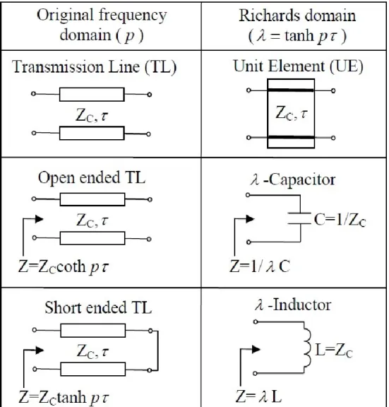
The transmission lines in 𝜆-domain of Richards transformation, can be treated as inductor if they are short circuited and as of capacitor if they are open circuited, in specific case if the length of transmission line is shorted then quarter of wavelength, as shown in Figure 2.3. So, the driving point impedance function of a network composed of open or short-circuited transmission lines, is real and positive rational function of 𝜆. Eventually, synthesis techniques used for lumped reactance two-port networks can be utilized for the networks built by commensurated transmission lines, In the case of cascaded connected transmission line, it has no lumped counterparts so must be dealt separately. This is the reason that the two-port equivalent network of transmission line in 𝜆-domain is taken as a unite element (UE).

(34)

19

Figure 2.3 Representation of transmission line unit elements and their counterparts in Richards transformation (ŞENGÜL, 2006).

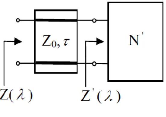
The networks functions of UEs based networks are clearly are the functions of 𝜆. The input impedance 𝑍(𝜆) of a unit element terminated network with another impedance 𝑍′_{(𝜆) can be} expressed as, 𝑍(𝜆) = 𝑍₀𝑍 ′_{(𝜆) − 𝜆𝑍} 0 𝜆𝑍′_{(𝜆) + 𝑍} 0 (2.49)

here 2.49 shows that if 𝑍′_{(𝜆) is rational then 𝑍(𝜆) will be rational as well. Conclusion can be} give as (ŞENGÜL, 2006) (Aksen, 1994),

(35)

20

• The driving point impedance of a distributed network composed of cascaded UEs is a positive real rational function of 𝜆.

By Richards theorem, UE of characteristic impedance 𝑍₀ = 𝑍(1) may always be obtained from the positive real impedance function 𝑍(𝜆) as in 2.49 and the expression became,

𝑍′(𝜆) = 𝑍(1)𝑍(𝜆) − 𝜆𝑍(1)

𝑍(1) − 𝜆𝑍(𝜆) (2.50)

𝑍′(𝜆) is also a positive real function with degree not higher than that of 𝑍(𝜆) in Figure 2.4. Moreover, for 𝐸𝑣 𝑍(𝜆)|_𝜆=1 = 0 in that case the degree of 𝑍′_{(𝜆) will be one less than 𝑍(𝜆). A} very similar expression of the theorem can also be given for the input reflection function (Carlin, 1971).

Figure 2.4 Application of Richards theorem.

2.6 Network Composed of Mixed Elements (Lumped and Distributed)

Working with waves of micro and millimeter frequency range, for circuit realization the use of lumped component only, causes serious implementation difficulties, these problems are physical interconnection of components and parasitic effects. To resolve these problems distributed structures made up of transmission line are used between the lumped element, these transmission lines are also helpful for design problems to improve the performance. A very

(36)

21

useful model can be concluded by the cascaded network of two-port reciprocal networks connected by mean of equal delayed ideal transmission lines.

In literature, designing of mixed lumped and distributed element was very important and has grasped attention for long time but still not able to develop and complete design theory for mixed lumped and distributed elements. Although some concepts of classical network theory have been used to design some types of mixed element two-port networks but not able to do approximation and synthesis of all arbitrary mixed element completely.

In the literature, work and devotion can be observed specifically for the mixed elements networks composed of lumped reactance and uniform ideal transmission lines (lossless and uniform). The idea is, cascaded lossless lumped two-ports connected with ideal transmission lines (UEs) (ŞENGÜL, 2006) (Aksen, 1994).

Matching networks and microwave filters are composed of this kind of cascaded structures. It is so obvious that they have properties of both lumped and distributed networks. These structures also offer advantages over those networks, designed only by transmission lines or lumped elements alone, harmonic filtering property is the most important benefit of the mixed structure. Furthermore, the physical circuit interconnections are made by nonredundant transmission line elements, help and contribute to the filtering performance of the structure.

(37)

22

3 A SEMI-ANALYTIC PROCEDURE FOR DESCRIBING LOSSLESS

TWO-PORT MIXED (LUMPED AND DISTRIBUTED ELEMENT)

NETWORKS

This chapter is committed to initiating the fundamental concepts and description of two-variable cascaded mixed (lumped and distributed elements) networks. Two-two-variable characterization of mixed cascades will be encountered and the discussion on the problems related to the creation of network functions with two variables will be studied, based on scattering parameters.

3.1 Two Variable Characterization of Cascaded Mixed Elements (Lumped

and Distributed) Two-port Networks

In several engineering problems, complex function with multivariable are commonly used to describe the response of a system. Design of a micro wave lossless two-port network constituted mixed lumped-distributed elements can be considered as a best example as designing of microwave lossless two-ports composed of mixed lumped-distributed elements. A microwave filter or a matching network may contain equal length transmission lines as well as lumped elements. To work with these kind of problems, the lumped sections of problems are expressed in terms of the complex frequency variable 𝑝 and the distributed section is described by using Richards variable λ = tanh 𝑝𝜏. To describe this system mathematically, a complex two variable function is used. Indeed, both complex variables λ and 𝑝 are hyperbolically dependent so that makes it a single variable problem. However, if we assume that both complex variables λ and 𝑝 are independent then it can be solved as two variable problem (Koga, 1971). KOGA has studied the existence of a relationship between multivariable and a certain class of single-variable transcendental functions (Koga, 1971). His work is redesigned for two-variable case is as follows;

• A rational multivariable function 𝑆(𝑝, 𝜆) is bounded if and only if the single variable function 𝑆(𝑝, λ = tanh 𝑝𝜏) is bounded for all 𝜏.

(38)

23

Two variable scattering matrix representation of a lossless two-ports composed of mixed lumped-distributed elements is 𝑆(𝑝, 𝜆) and transfer scattering matrix representation is 𝑇(𝑝, 𝜆). The canonic representation of 𝑆(𝑝, 𝜆) and 𝑇(𝑝, 𝜆), in terms of two-variable polynomials 𝑔(𝑝, 𝜆), ℎ(𝑝, 𝜆), and 𝑓(𝑝, 𝜆) is (Fettweis, 1982); 𝑆(𝑝, 𝜆) = 1 𝑔(𝑝, 𝜆) [ ℎ(𝑝, 𝜆) 𝜎𝑓(−𝑝, −𝜆) 𝑓(𝑝, 𝜆) −𝜎ℎ(−𝑝, −𝜆)] (3.1) 𝑇(𝑝, 𝜆) = 1 𝑓(𝑝, 𝜆)[ 𝜎𝑔(−𝑝, −𝜆) ℎ(𝑝, 𝜆) 𝜎ℎ(−𝑝, −𝜆) 𝑔(𝑝, 𝜆) ] (3.2)

The properties of canonic polynomial 𝑓, 𝑔, 𝑎𝑛𝑑 ℎ are given as (Aksen, 1994) (ŞENGÜL, 2006).

1. 𝑔(𝑝, 𝜆) ≠ 0 for Re {𝑝, 𝜆} > 0,

2. 𝑔(𝑝, 𝜆) ≠ 0 is relatively prime with 𝑔(−𝑝, −𝜆).

• 𝑓 = 𝑓(𝑝, 𝜆), 𝑔 = 𝑔(𝑝, 𝜆) and ℎ = ℎ(𝑝, 𝜆) are real polynomials in complex frequency domain.

• The relation between 𝑓, 𝑔 and ℎ is,

𝑔(𝑝, 𝜆)𝑔(−𝑝, −𝜆) = ℎ(𝑝, 𝜆)ℎ(−𝑝, −𝜆) + 𝑓(𝑝, 𝜆)𝑓(−𝑝, −𝜆) (3.3) • 𝜎 is constant with value ±1.

• If two-port network includes UEs, then the definition of 𝑓 will be,

𝑓(𝑝, 𝜆) = 𝑓(𝑝)𝑓(𝜆) = 𝑓(𝑝)𝑓(1 − 𝜆2)𝑛𝜆⁄2 (3.4)

where 𝑛𝜆 is showing the number of unit elements UEs.

In the upcoming sections, the discussion on the cascades of mixed lumped and distributed two-port lossless networks is entirely based on the canonic representation of scattering matrix.

(39)

24

3.1.1 Basic Definitions and Properties

In this section, to get understanding and awareness about common terminologies, some fundamental definitions will be introduced to represent the properties of lossless two-port networks made up of mixed lumped and distributed elements.

3.1.1.1 Lossless Lumped ladder

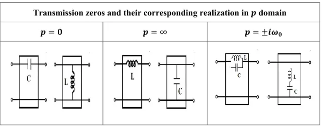
Definition 1: A lossless two-port, consists of just a single transmission zero in 𝑝 domain will

be referred to as simple lumped section (SLS).

The transmission zeros of the SLS on the finite 𝑖𝜔-axis are located at 𝑝 = 0 , 𝑝 = ∞ and 𝑝 = 𝑖𝜔 and realization of the concept is shown in Figure 3.1. The point should be noted that the transmission zeroes of 𝑖𝜔-axis must always be present with its complex conjugate as a pair. To fulfill the practical desires, transmission zeroes at 𝑝 = 0 and/or 𝑝 = ∞ are preferred to be work with.

Transmission zeros and their corresponding realization in 𝒑 domain

𝒑 = 𝟎 𝒑 = ∞ 𝒑 = ±𝒊𝝎𝟎

Figure 3.1 Simple Lumped Section.

Definition 2: Cascaded connection of SLS, consists of just 𝑖𝜔 transmission zeros in 𝑝 domain

(40)

25

Belevitch’s scattering representation of an LLL network is,

𝑆(𝑝) = 1 𝑔(𝑝) [

ℎ(𝑝) 𝜎𝑓(−𝑝)

𝑓(𝑝) −𝜎ℎ(−𝑝)] (3.5)

The properties of canonic real polynomial 𝑓(𝑝), 𝑔(𝑝), 𝑎𝑛𝑑 ℎ(𝑝) are given as (Aksen, 1994) (ŞENGÜL, 2006).

• 𝑓 = 𝑓(𝑝), 𝑔 = 𝑔(𝑝) and ℎ = ℎ(𝑝) are real polynomials in complex frequency domain.

• The relation between 𝑓, 𝑔 and ℎ is,

𝑔(𝑝)𝑔(𝑝) = ℎ(𝑝)ℎ(−𝑝) + 𝜎𝑓2(𝑝) (3.6)

• 𝜎 is constant and 𝑓(𝜎 = ±1).

Equation 3.6 in turn imply following degree relations,

deg ℎ ≤ deg 𝑔 𝑎𝑛𝑑 deg ℎ ≤ deg 𝑓 (3.7) The term deg 𝑔 − deg 𝑓 is representing the number of transmission zeros at infinity and the information about the degree of lossless two-port network lies and equal to the degree of polynomial 𝑔.

Consider 𝑛𝑝 = deg 𝑔 and the coefficient form of 𝑓(𝑝), 𝑔(𝑝), 𝑎𝑛𝑑 ℎ(𝑝).

𝑓(𝑝) = ∑ 𝑓_𝑘𝑝𝑘 𝑛𝑝 𝑘=0 , ℎ(𝑝) = ∑ ℎ_𝑘𝑝𝑘 𝑛𝑝 𝑘=0 , 𝑔(𝑝) = ∑ 𝑔_𝑘𝑝𝑘 𝑛𝑝 𝑘=0 (3.8)

(41)

26

In 3.8 all the polynomials are considered as of degree 𝑛𝑝 for the sake of convenience to formulate the upcoming equations. From 3.7, the inequality relations of degree of polynomial that if deg 𝑓 < 𝑛𝑝 and deg ℎ < 𝑛𝑝 one must set corresponding coefficient of the polynomial ℎ and 𝑓 equal to zero. Consider 3.6 which led us to,

𝐹(−𝑝2) = 𝑓(𝑝)𝑓(−𝑝) = ∑ 𝑓𝑘𝑝2𝑘 𝑛𝑝 𝑘=0 𝐻(−𝑝2) = ℎ(𝑝)ℎ(−𝑝) = ∑ ℎ_𝑘𝑝2𝑘 𝑛𝑝 𝑘=0 𝐺(−𝑝2) = 𝑔(𝑝)𝑔(−𝑝) = ∑ 𝑔𝑘𝑝2𝑘 𝑛𝑝 𝑘=0 (3.9)

The coefficient of 𝐹_𝑘 , 𝐺_𝑘 and 𝐻_𝑘 can be given as,

𝐹_𝑘= ∑ 𝑓𝑙𝑓2𝑘−𝑙 , 2𝑘 𝑙=0 𝐺𝑘 = ∑(−1)2𝑘−𝑙𝑔𝑙𝑔2𝑘−𝑙 , 2𝑘 𝑙=0 𝐻𝑘= ∑(−1)2𝑘−𝑙ℎ𝑙ℎ2𝑘−𝑙 2𝑘 𝑙=0 (3.10)

where set the values of 𝑓𝑙 = 𝑔𝑙 = ℎ𝑙 = 0 for 𝑙 > 𝑛𝑝 and by using the relationship in 3.10 the lossless relation in 3.6 can be given as,

𝐺(−𝑝2_{) = 𝐻(−𝑝}2_{) + 𝐹(−𝑝}2₎ _(3.11) The following set of 𝑛_𝑝+ 1 quadratic equations can be obtained.

𝑔₀2 _{= ℎ} 02+ 𝑓02 𝑔_𝑘2 + 2 ∑(−1)𝑘−𝑙_𝑔 𝑙𝑔2𝑘−𝑙 𝑘−𝑙 𝑙=0 = ℎ_𝑘2+ 𝑓_𝑘2+ 2 ∑(−1)𝑘−𝑙_(ℎ 𝑙ℎ2𝑘−𝑙+ 𝑓𝑙𝑓2𝑘−𝑙) 𝑘−𝑙 𝑙=0

⋮

for 𝑘 = 1,2, … , 𝑛_𝑝− 1 𝑔_𝑛2_𝑝 _{= ℎ} 𝑛𝑝 2 _{+ 𝑓} 𝑛𝑝 2 (3.12)

(42)

27 where set the values of 𝑓𝑙 = 𝑔𝑙= ℎ𝑙= 0 for 𝑙 > 𝑛𝑝. 3.1.1.2 Cascaded Distributed Section

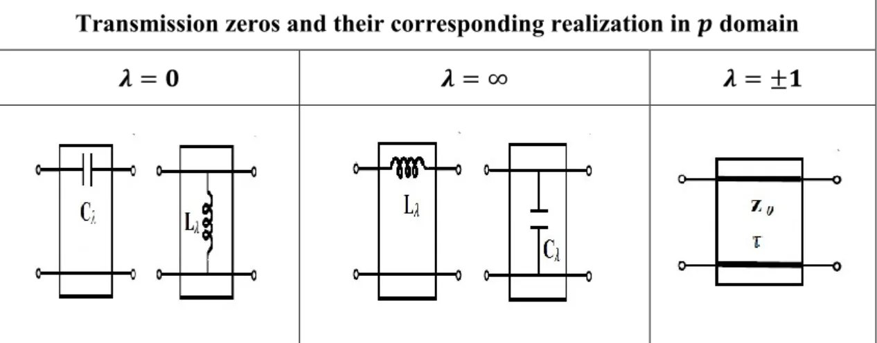
Definition 1: A lossless two-port network, consists of just a single transmission line of

characteristic impedance 𝑍₀ and delay length 𝜏 is called a simple distributed section (SDS).

It is clear now, that SDS may include a unit element or open or short remnant in series or shunt configuration. Figure 3.2 is a depiction of the Richard’s domain realization and transmission zeroes associated with simple distributed section and here open stubs are represented by 𝜆-capacitors and short stubs are represented by 𝜆-inductors.

Transmission zeros and their corresponding realization in 𝒑 domain

𝝀 = 𝟎 𝝀 = ∞ 𝝀 = ±𝟏

Figure 3.2 Simple Distributed Section.

Definition 2: Cascaded connection of equal length SDS, will be referred to as cascaded distributed section (CDS).

Definition 3: A CDS, that consist of only commensurated UEs, will be called as cascaded UE section (CUS).

Generally, a normal CDS can be expressed in term of its bounded real scattering parameters by using Richard’s variable 𝜆. In this case, 𝑝 will be changed into 𝜆 in 3.5, expression for canonic polynomial representation and a factor 𝑓(1 − 𝜆2₎1⁄₂_{will be introduced in polynomial 𝑓(𝜆) as} explained in earlier sections.

(43)

28

𝑓(𝜆) = 𝑓₀(𝜆)𝑓(1 − 𝜆2₎𝑛⁄₂ _(3.13) where 𝑓₀(𝜆) is real polynomial could be even or odd and 𝑛 is showing the number of UEs in cascade.

Like the lumped element case, CDS can also be expressed completely in terms of ℎ(𝜆) if 𝑓(𝜆) is preselected. So 3.6 can be written as,

𝑔(𝜆)𝑔(−𝜆) = ℎ(𝜆)ℎ(−𝜆) + 𝜎𝑓2_{(𝜆)𝑓(1 − 𝜆}2₎𝑛 _(3.14) where 𝜎 is constant, as expressed earlier.

Consider all the polynomials 𝑔(𝜆), ℎ(𝜆) and 𝑓(𝜆) are of degree 𝑛𝜆 for the sake of convenience to formulate the upcoming equations. If ℎ(𝜆) and 𝑓(𝜆) are known then the value of 𝑔(𝜆) can be estimated explicitly by factorization of 𝑔(𝜆)𝑔(−𝜆) given in 3.14 or by solving set of quadratic equations, can be derived in similar manner as of lumped case discussed above,

𝑔₀2 _{= ℎ} 02+ 𝑓02 𝑔_𝑘2 + 2 ∑(−1)𝑘−𝑙_𝑔 𝑙𝑔2𝑘−𝑙 𝑘−𝑙 𝑙=0 = ℎ_𝑘2+ 𝑓_𝑘2+ 2 ∑(−1)𝑘−𝑙_(ℎ 𝑙ℎ2𝑘−𝑙+ 𝑓𝑙𝑓2𝑘−𝑙) 𝑘−𝑙 𝑙=0

⋮

for 𝑘 = 1,2, … , 𝑛_𝜆 − 1 𝑔𝑛𝜆 2 _{= ℎ} 𝑛𝜆 2 _{+ 𝑓} 𝑛𝜆 2 (3.15)

where set the values of 𝑓_𝑙 = 𝑔_𝑙= ℎ_𝑙= 0 for 𝑙 > 𝑛_𝜆. 𝑔(𝜆) is strictly Hurwitz polynomial.

The above discussion can be concluded in following points.

• Any LLL and CDS can completely described in terms of real coefficient of ℎ polynomial, if 𝑓 is known in advance. To achieve the desire goal, carry out Hurwitz factorization to generate 𝑔 a strictly Hurwitz polynomial.

• There is another alternative method to generate 𝑔, a strictly Hurwitz polynomial. In this method a set of quadratic equation is obtained by solving the losslessness equation 3.6 and 3.14, and solve them to get 𝑔.

(44)

29

• In the above formulations of transfer scattering function, the numerator polynomial 𝑓(𝜆) or 𝑓(𝑝) imposes restricted class of topologies such as ladder or cascaded distributed section. Despite the selective choice of 𝑓(𝜆) or 𝑓(𝑝), still there is a possibility of ending up with different circuit configurations with in the past class topologies.

• While in working with one kind of network elements, either only lumped elements or only commensurate transmission line and synthesis procedures are well established in 𝜆 or 𝑝 domain. The synthesis can easily be completed by extracting the transmission zeros, which in turn yields a degree reduction in the driving point function. In this case, the driving point function may be expressed as a reflection or immittance function, in Darlington sense. Extraction of simple transmission zeros from a given driving point function is equivalent to the extraction of a simple selection. In this type of cascade synthesis procedure, it is not necessary to have the knowledge about how the simple

section are connected to each other. The information about the connection is imbedded

in the synthesis procedure, in the realization of single variable driving point function.

3.1.2 Cascaded Lumped-Distributed Two-Port Networks

Definition 1: A lossless two-port network, that consist of cascade connection of simple lumped

section and commensurated length simple distributed sections, is known as cascaded

lumped-distributed two-port (CLDT).

Definition 2: A special cascaded lumped-distributed two-port, that is formed by employing

commensurate length UEs placed between the elements of an LLL referred to as low-pass

ladder with UEs (LPLU). Here an assumption has been made that the low-pass type LLL

includes the transmission zeros only at ∞.

A CLDT can be represented by using the two-variable scattering parameters, function of complex frequency variable 𝜆 and 𝑝. The scattering matrix representation of a CLDT can be denoted as 𝑆 = 𝑆(𝑝, 𝜆) and for scattering transfer matrix 𝑇 = 𝑇(𝑝, 𝜆). The Belevitch’s canonic representation in terms of two variable polynomial is as 𝑓 = 𝑓(𝑝, 𝜆), 𝑔 = 𝑔(𝑝, 𝜆) and ℎ = ℎ(𝑝, 𝜆)follows,

(45)

30 𝑆 = 1 𝑔[ ℎ 𝜎𝑓_∗ 𝑓 −𝜎ℎ_∗] 𝑎𝑛𝑑 𝑇 = 1 𝑓[ 𝜎𝑔_∗ ℎ 𝜎ℎ_∗ 𝑔] (3.16)

where 𝑓_∗ = 𝑓(−𝑝, −𝜆) is paraconjugate of a real function. The properties of canonic polynomial 𝑓, 𝑔, 𝑎𝑛𝑑 ℎ are given as (Aksen, 1994) (ŞENGÜL, 2006).

• 𝑓 is monic, i.e. its leading coefficient is equal to unity. • 𝜎 is constant and 𝜎 = ±1.

• 𝑔 is strictly Hurwitz polynomial. 1. 𝑔(𝑝, 𝜆) ≠ 0 for Re {𝑝, 𝜆} > 0,

2. 𝑔(𝑝, 𝜆) ≠ 0 is relatively prime with 𝑔(−𝑝, −𝜆).

• 𝑓, 𝑔 and ℎ are real polynomials with complex variable 𝜆 and 𝑝. • The relation between 𝑓, 𝑔 and ℎ is,

𝑔𝑔_∗ = 𝑓𝑓_∗+ ℎℎ_∗ (3.17)

• If two-port network includes UEs, then the definition of 𝑓 will be,

𝑓 = 𝑓0(𝑝, 𝜆)𝑓(1 − 𝜆2) 𝑛

2

⁄ _(3.18)

where 𝑢 is showing the number of unit elements UEs.

3.1.2.1 Connectivity Information Cascaded Lumped-Distributed Two-Port Networks

It is proven fact that canonic representation of two-variable network is possible (Fettweis, 1982). As for as the realizability conditions are concerned, it has also been asserted that scattering matrix satisfying the conditions explained in earlier sections (Aksen, 1994). While working with the case of cascaded topology, to insure the realizability and practicability as a cascade network then the scattering matrix and its canonic polynomial with two variables must satisfy some more conditions. The most intuitive way to apply these extra conditions for cascaded structures is to study the effect of the topologic constraints and restrictions on the polynomial form. To achieve our purpose, some properties of the polynomials 𝑓, 𝑔 and ℎ related to cascaded lumped-distributed two-port are discussed as follows,

(46)

31

Let’s start with the introductory notations and fundamental definition related to the two-variable polynomials, will be used in upcoming discussion. A two two-variable polynomial say, 𝑔 = 𝑔(𝑝, 𝜆), its coefficient form will be,

𝑔(𝑝, 𝜆) = ∑ ∑ 𝑔_𝑘𝑙𝑝𝑙_𝜆𝑘 𝑛𝑝 𝑙=0 𝑛𝜆 𝑘=0 (3.19)

where 𝑛_𝜆 is a partial degree of 𝑔 in the variables 𝜆 and 𝑛_𝑝 is partial degrees of 𝑔 in the variables 𝑝. The arrangement shown in 3.19 can also be rearrange and written as,

𝑔(𝑝, 𝜆) = ∑ 𝑔_𝑘(𝜆)𝑝𝑘_{= ∑ 𝑔} 𝑘(𝑝)𝜆𝑘 𝑛𝜆 𝑘=0 𝑛𝑝 𝑘=0 (3.20)

There is another form to represent a two-variable polynomial is,

𝑔(𝑝, 𝜆) = 𝐩𝐓_𝐀 𝐠𝛌 = 𝛌𝐓𝐀𝐠𝐩 (3.21) where 𝐀_𝐠 = [ 𝑔00 𝑔01 𝑔10 𝑔11 ⋯ 𝑔_0𝑛_𝜆 𝑔_1𝑛_𝜆 ⋮ ⋱ ⋮ 𝑔_𝑛_𝑝₀ 𝑔_𝑛_𝑝₁ _{⋯ 𝑔} 𝑛𝑝𝑛𝜆 ] , 𝑝 = [ 1 𝑝 𝑝2 ⋮ 𝑝𝑛𝑝_] 𝑎𝑛𝑑 𝜆 = [ 1 𝜆 𝜆2 ⋮ 𝜆𝑛𝜆] (3.22)

Definition 1: The highest power of a variable, with non-zero coefficient is the definition of a

two-variable polynomial 𝑔 = 𝑔(𝑝, 𝜆), i.e. 𝑛_𝑝 = deg_𝑝𝑔(𝑝, 𝜆) and 𝑛_𝜆 = deg_𝜆𝑔(𝑝, 𝜆).

Definition 2: The absolute total degree of a two-variable polynomial 𝑔(𝑝, 𝜆) with partial

degrees 𝑛𝑝and 𝑛𝜆, will be equal to the sum of these partial degrees and mathematically can be expressed as,

(47)

32

𝑛 = 𝑚𝑎𝑥_𝑔_𝑘𝑙≠0{𝑘 + 𝑙} 𝑘 = 0,1, … , 𝑛𝑝 , 𝑙 = 0,1, … , 𝑛𝜆 (3.23) Now from a cascaded topology consider the transmission zeroes. It is critical to select and appropriate 𝑓(𝑝, 𝜆) function for a mixed lumped-distributed two-port, because 𝑓(𝑝, 𝜆) includes transmission zeros, which in turn enforce topological restrictions on the loss two-port constructed with lumped elements and commensurated distributed elements.

In a mixed element design composed of cascaded connection of 𝑛_𝑝 lumped and 𝑛_𝜆 distributed elements. The polynomial 𝑓(𝑝, 𝜆) can be given as,

𝑓(𝑝, 𝜆) = ∏ 𝑓_𝑘(𝑝) 𝑓𝑘(𝜆) 𝑛

𝑘=1

(3.24)

where 𝑓𝑘(𝑝) and 𝑓𝑘(𝜆) interpret the transmission zeros of discrete lumped and distributed subsegments present in the cascade. Generally, the transmission zeros can possess any place in the 𝑝 and 𝜆 plane. From 3.24, an immediate conclusion can be drawn, that in the cascade the transmission zeros in each subsegment have to appear in multiplication form. In simple words, the polynomial 𝑓(𝑝, 𝜆) of whole mixed element network can be assumed as product separable form,

𝑓(𝑝, 𝜆) = 𝑓′(𝑝)𝑓′′(𝜆) (3.25)

𝑓′_{(𝑝) will be a real even or odd polynomial if the transmission zeroes are considered on the} imaginary axis 𝑖𝜔 or 𝑖Ω, and general expression for 𝑓′′_{(𝜆) is,}

𝑓′′(𝜆) = 𝑓₀(𝜆)𝑓(1 − 𝜆2₎𝑛⁄₂ _(3.26) where 𝑢 is indication the number of UEs present in the principal path from input to output of CLDT. By overlooking the zeros of the finite imaginary axis in 𝑓′_{(𝜆) and 𝑓}′′_(𝜆) (𝑒𝑥𝑐𝑙𝑢𝑑𝑖𝑛𝑔 𝑡ℎ𝑜𝑠𝑒 𝑎𝑡 𝑑𝑐), a realistic form of 𝑓(𝑝, 𝜆) can be derived as,

(48)

33

here total number of transmission zeros at dc of the lumped and distributed are represented by 𝑞₁ and 𝑞₂ respectively. After excluding the transmission zeros at dc, the expression in 3.27 can be written as,

𝑓(𝑝, 𝜆) = 𝑓(1 − 𝜆2)𝑛⁄2 (3.28)

This is the characteristic configuration of 𝑓(𝑝, 𝜆) of an LPLU design composed of simple lumped elements and UEs. It is clear in this case that 𝑓(𝑝, 𝜆) is only dependent function of 𝜆 . Matrix representation of the real coefficients of 𝑔(𝑝, 𝜆) and ℎ(𝑝, 𝜆) is,

𝐀𝒉= [ ℎ₀₀ ℎ₀₁ ℎ₁₀ ℎ₁₁ ⋯ ℎ_0𝑛_𝜆 ℎ_1𝑛_𝜆 ⋮ ⋱ ⋮ ℎ_𝑛_𝑝₀ ℎ_𝑛_𝑝₁ _⋯ _ℎ_𝑛 𝑝𝑛𝜆] , 𝐀𝐠 = [ 𝑔00 𝑔01 𝑔₁₀ 𝑔₁₁ ⋯ 𝑔_0𝑛_𝜆 𝑔_1𝑛_𝜆 ⋮ ⋱ ⋮ 𝑔_𝑛_𝑝₀ 𝑔_𝑛_𝑝₁ _⋯ _𝑔 𝑛𝑝𝑛𝜆 ] (3.29)

Property 1: The two-variable polynomial 𝑔(𝑝, 𝜆), ℎ(𝑝, 𝜆) and 𝑔(𝑝, 𝜆) can be expressed in

term of a single variable 𝑝 by putting 𝜆 = 0, the lumped lossless two-port in this case can be completely described by columns of 𝐀𝒉 matrix.

Property 2: The two-variable polynomial 𝑔(𝑝, 𝜆), ℎ(𝑝, 𝜆) and 𝑔(𝑝, 𝜆) can be expressed in

term of a single variable 𝜆 by putting 𝑝 = 0, the lumped lossless two-port in this case can be completely described by rows of 𝐀𝒉 matrix.

According to the above properties, it can be proved that the coefficient matrices 𝐀_𝒉 and 𝐀_𝒈 can

entirely be generated by using first column and first row of matrix 𝐀_𝒉, if the information about the cascaded connection is pre-known, while assuming the cascaded connections of lumped and distributed two-ports structures, in alternating order. This claim can be proved by considering following assumption,

(49)

34

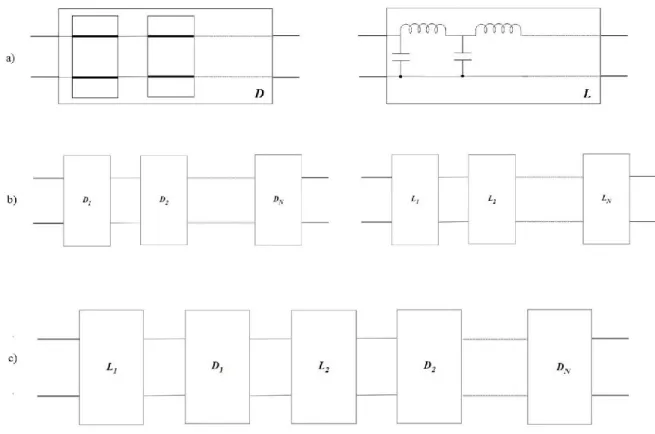
Figure 3.3 a) Cascaded Distributed Design and Lossless Lumped Ladder. b) Cascaded Decomposition. c)Cascade of Simple Lumped and Distributed Section.

Consider Figure 3.3(a) where L is representing LLL (lossless lumped ladder) and D is denoting CSD (cascaded distributed section). With the help of algebraic network decomposition

technique (Aksen, 1994) the network present in Figure 3.3 can be decomposed into their Lk and Dk subsections as depicted in Figure 3.3(a). Now consider Figure 3.3(c), in which a lossless two-port network is constructed by using alternating ordered cascade connections of lumped and distributed subsections.

Assume that 𝑆(𝜆) and 𝑆(𝑝) are respectively representing the scattering matrix 𝑆(𝑝, 𝜆)of cascaded distributed section D and lossless lumped ladder L. In this representation, the scattering matrix of the developed mixed composition, can be determined in terms of scattering matrices of subsections 𝑆𝑘(𝜆) and 𝑆𝑘(𝑝), determine from 𝑆(𝜆) and 𝑆(𝑝) respectively. While working on the decomposition of 𝑆(𝜆) and 𝑆(𝑝), the number of elements and the corresponding zeros of transmission are designer’s choice for every subsegment, after these selections with