T.C.
SELÇUK ÜNİVERSİTESİ FEN BİLİMLERİ ENSTİTÜSÜ
COMPARISON OF DATA
REDUCTIONALGORITHMS FOR BIOMEDICAL APPLICATIONS
Thibaut Judicael BAH
MS THESIS
Computer Engineering Department
Supervisor: Prof. Dr. Bekir KARLIK June-2015
KONYA All Right Reserved
Thibaut Judicael BAH tarafindan hazırlanan “Biyomedikal Uygulama için Veri Azaltma Algoritmaları Karşılaştırılması” adlı tez çalıması 10/06/2015 tarihinde aşağıdaki jüri tarafindan oy birliği ile Selçuk Üniversitesi Fen Bilimleri Enstitüsü Bilgisayar Mühendisliği Anabilim Dalı’nda YÜKSEK LİSANS TEZİ olarak Kabul edilmiştir.
Jüri Üyeleri İmza
Başkan
Doç.Dr. Halife KODAZ ………..
Danışman
Prof.Dr. Bekir KARLIK ……….. Üye
Doç.Dr. Halis ALTUN ………..
Yukarıdaki sonucu onaylarım.
Prof.Dr. Aşır Genç FBE Müdürü
Bu tezdeki bütün bilgilerin etik davranış ve akademik kurallar çerçevesinde elde edildiğini ve tez yazım kurallarına uygun olarak hazırlanan bu çalışmada bana ait olmayan her türlü ifade ve bilginin kaynağına eksiksiz atıf yapıldığını bildiririm.
DECLARATION PAGE
I hereby declare that all information in this document has been obtained and presented in accordance with academic rules and ethical conduct. I also declare that, as required by these rules and conduct, I have fully cited and referenced all material and results that are not original to this work.
İmza
Thibaut Judicael BAH 10/06/2015
YÜKSEK LİSANS TEZİ
BİYOMEDİKAL UYGULAMA İÇİN VERİ AZALTMA ALGORİTMALARI KARŞILAŞTIRILMASI
Thibaut Judicael BAH
Selçuk Üniversitesi Fen Bilimleri Enstitüsü Bilgisayar Mühendisliği Anabilim Dalı
Danışman: Prof.Dr. Bekir KARLIK
2015, 83 Sayfa Jüri
Prof.Dr. Bekir KARLIK Doç.Dr. Halife KODAZ
Doç.Dr.Halis ALTUN
Tıpta yumuşak hesaplama yöntemi birkaç yıldır büyüyen bir alandır. Biyoinformatik araştırmada ilerlemeye giderek, ve aynı zamanda karmaşık, büyük ve çok boyutlu verisetlerine bakan. Örneğin, yönbağımlı doğrusal olmayan difüzyon ile biyomedikal ve yapısal hücre biyolojisi 3 boyut görüntülerden ilgisiz verilerin ortadan kaldırılması hesaplamada pahalı. ECG Holter kaydedildi ve görevi öğrenmek için 100 binden fazla kalp atışları saklanan, hangi bilgiyi değerlendirecek ve daha sonra nihai bir çalışma veya test için tercih edilecegi hangi kalp atışları belirlenecegi zor bir iştir; bir hesaplama açısından pahalı ve büyük bir bellek alanı gerektirir [1].
Tıbbi görüntülerde hastadan hastaya birçok ortak özellik sunmak, ancak aralarındaki farklılıklar her zaman bazı anormalliklere neden olmayabilir. Bu tür görüntüler için biçimi çeşitli görüntü işleme başarı sınırlayan bir karmaşıklığa yol açar.
Veri azaltma hedefliyor işlenecek konuyu kolay hale getirmek için de orijinal veri kümesinden gereksiz verileri ortadan kaldırmaktır. Veri azaltılması için etkili bir yaklaşımdır. Dahası, etkin biyoinformatik uygulamalarında önemli bir işlemdir.
Anahtar Kelimeler: Biyoinformatik, Özellik seçimi, Veri azaltma,Veri indirgeme, Veri madenciliği, Yumuşak hesaplama.
MS THESIS
COMPARISON OF DATA REDUCTIONALGORITHMS FOR BIOMEDICAL APPLICATIONS
Thibaut Judicael BAH
SELCUK UNIVERSITY SCIENCE INSTITUTE COMPUTER ENGINEERING DEPARTMENT
Advisor: Prof.Dr. Bekir KARLIK 2015, 83 Pages
Jury
Prof.Dr. Bekir KARLIK Assoc.Prof. Halife KODAZ
Assoc.Prof. Halis ALTUN
The soft computing method in medicine is a growing field for several decades. Bioinformatics research advance increasingly, and facing at the same time complex, complicated, large and multidimensional datasets.For example; removing irrelevant data from 3 dimensions images in biomedicine and structural cellular biology by Anisotropic nonlinear diffusion is computationally expensive.
ECG Holter recorded and stored more than 100 thousand heartbeats for it learning task, which is a difficult work to evaluate the information and then determine which heartbeats are to be choose for an eventual study or test; from a computational perspective it is costly and require a large memory space [1].
Medical images present many common features from patient to patient but the differences between them may not always be due to some abnormality. This variety of format for such images leads to a complexity that restricts the success of image processing.
Data reduction aims is toremove the irrelevant data, reduce the dimensionality, the instances, the redundancy and the complexity of a dataset in order to make it easy to be processed. It is an efficacious approach for data reduction. Moreover, it is a crucial procedure in effective bioinformatics applications.
Keywords:Bioinformatics, Data mining, Data reduction, Feature selection, Instance reduction, Soft computing.
I would like to begin by expressing my deep gratitude to the one who in the past two years has been for me a father, a mentor, an advisor; the Prof.DrBekirKarlik my supervisor who supported me intellectually during the writing of my thesis.
I thank my family, especially my father and my mother for their moral support that has been a great solace throughout these years of hard work.
I would also like to thank all those who make me the honour of their friendship, I could mention among otherZunonCyrille, Augusta Wicaksono, Alaa Hamid, Desire AnnickKouman, Martel Makwemba and BurakDere. I have been blessed by your presence in my life.
Thibaut Judicael BAH KONYA-2015
v
TABLE OF CONTENTS
ABSTRACT ... viii
ACKNOWLEDGEMENT ... ix
TABLE OF CONTENTS ... v
LIST OF TABLES ... viii
LIST OF FIGURES ... ix
LIST OF SYSMBOLS AND ABBREVIATIONS ... xi
1. INTRODUCTION ... 2
1.1. Organization of Thesis ... 3
1.2. Literature Survey ... 4
2. DATA MINING: CONCEPTS AND DEFINITIONS ... 6
2.1. Definition ... 6 2.2. Representation of Data ... 7 2.3. Learnıng Algorıthms ... 8 2.3.1. Naive bayes ... 9 2.3.2. C4.5 decision tree ... 11 2.3.3. K-Nearest neighbours ... 13
2.3.4. Artificial neural networks (ANN) ... 14
2.4. Performance Assessment ... 17
2.5. Weka Toolbox ... 18
3. FEATURE SUBSET SELECTION ... 20
3.1. Pattern Recognıtıon And Feature Selectıon ... 21
3.2. Feature Selectıon Algorıthms ... 21
3.3. Heurıstıc Search ... 23
3.4. Wrapper Methods For Feature Selectıon ... 26
3.4.1. Wrapper using decision trees algorithms ... 27
3.4.2. Wrapper using naïve bayes classifier ... 28
vi
3.5. Fılter Methods For Feature Selectıon ... 30
3.5.1. Filters through consistency subset ... 30
3.5.2. Feature selection by discretization ... 32
3.5.3. Feature filter using information theory ... 32
3.5.3. Feature filter using instance based approach ... 34
4. INSTANCE REDUCTION ... 34
4.1. Wrapper Methods For Instances Reductıon ... 36
4.1.1. Wrapper methods based on the concept of nearest neighbors ... 36
4.1.2. Wrapper methods based on the concept of associate ... 37
4.1.3. Wrapper method based on Support Vector Machine ... 38
4.1.4. Wrapper methods based on Tabu and Sequential Search ... 39
4.2. Filter Methods For Instances Reduction ... 39
4.2.1. Filter methods based on border instances ... 39
4.2.2. Filter methods using clustering ... 40
4.2.3. Filter methods based on weights assigning ... 41
4.2.4. Filter methods based on sampling ... 41
5. APPLICATIONS ... 43
5.1. Data Reduction Techniques Applicatıons On Cardiotocography Dataset Using Machine Learning Algorithms ... 43
5.1.1. Materials and methods ... 44
5.1.1.1. Dataset ... 44
5.1.1.2. Data reduction algorithms ... 44
5.1.1.3. Learning algorithms ... 45
5.1.2. Application ... 45
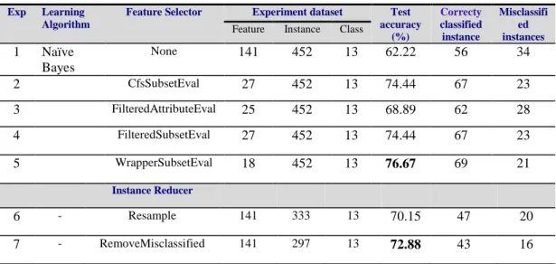
5.1.2.1. Experiments and results ... 46
5.2. Applicatıon of Data Reduction Algorithms on Parkinson Disease Dataset Using Machine Learning Algorithms ... 50
5.2.1. Materials and methods ... 50
5.2.1.1. Dataset ... 50
5.2.1.2. Data reduction algorithms ... 51
5.2.1.3. Learning algorithms ... 51
5.2.2. Application ... 52
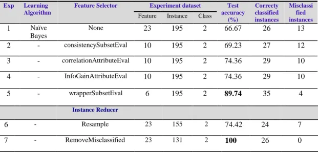
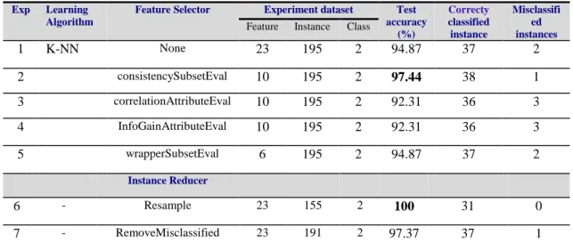
5.2.2.1. Experiments and results ... 52
5.3. A Study of Data Reduction Techniques Using Machine Learning Algorithms And Cardiac Arrhythmia Dataset ... 56
5.3.1. Materials and methods ... 56
5.3.1.1. Dataset ... 56
5.3.1.2. Data reduction algorithms ... 57
vii
5.3.2. Application ... 58
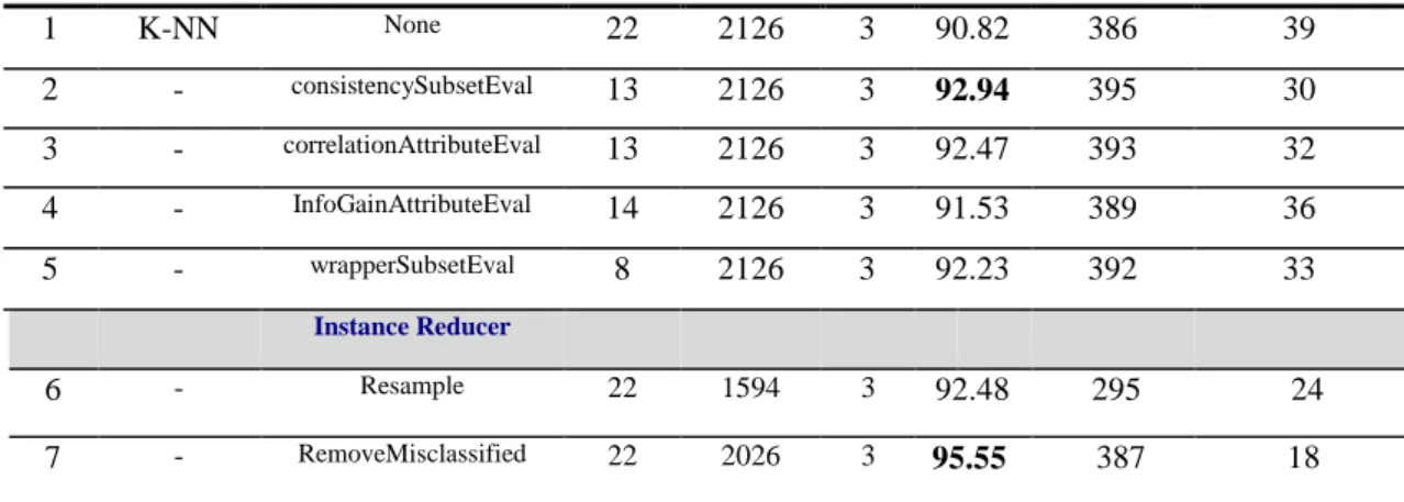
5.3.2.1. Experiments and results ... 58
6. CONCLUSIONS ... 62
6.1. Conclusıon ... 62
6.2. Future Work ... 62
BIBLIOGRAPHY ... 63
viii
LIST OF TABLES
2.1 Tennis dataset ... 8
2.2Correlation between features and classes of the tennis data ... 10
3.1Algorithm of Greedy Hill Climbing search ... 25
3.2 The Best First Search Algorithm ... 25
3.3 Simple genetic search strategy ... 26
5.1 Cardiotocography test results of original and reduced data using Naïve Bayes ... 47
5.2 Cardiotocography test results of original and reduced data using C4.5 decision tree ... 47
5.3 Cardiotocography test results of original and reduced data using K-NN ... 47
5.4 Cardiotocography test results of original and reduced data using ANN-MLP ... 47
5.5 Parkinson Disease test results of original and reduced data using Naïve Bayes ... 54
5.6 Parkinson Disease test results of original and reduced data using C4.5 decision tree ... 54
5.7 Parkinson Disease test results of original and reduced data using ANN-MLP ... 54
5.8 Parkinson Disease test results of original and reduced data using K-NN ... 55
5.9 Cardiac Arrhythmia test results of original and reduced data using C4.5 ... 59
5.10 Cardiac Arrhythmia test results of original and reduced data using Naïve Bayes ... 60
5.11 Cardiac Arrhythmia test results of original and reduced data using K-NN ... 60
5.12 Cardiac Arrhythmia test results of original and reduced data using ANN-MLP ... 60
ix
LIST OF FIGURES
2.1 Knowledge discovering in databases ... 7
2.2 Tennis data decision tree ... 12
2.3 General architecture of MLP ... 16
3.1 Wrapper and filter algorithms ... 23
3.2 Space of feature subset for the Tennis dataset ... 24
4.1 Instance reduction process ... 35
5.1 Cardiotocography test results comparison using Naïve Bayes as learning algorithm ... 49
5.2 Cardiotocography test results comparison using C4.5 as learning algorithm ... 49
5.3 Cardiotocography test results comparison using K-NN as learning algorithm ... 49
5.4 Cardiotocography test results comparison using ANN-MLP as learning algorithm ... 49
5.5 Parkinson Disease test results comparison using Naïve Bayes as learning algorithm ... 55
5.6 Parkinson Disease test results comparison using C4.5 as learning algorithm ... 55
5.7 Parkinson Disease test results comparison using ANN-MLP as learning algorithm ... 56
5.8 Parkinson Disease test results comparison using K-NN as learning algorithm ... 56
5.9 Cardiac Arrhythmia test results comparison using C4.5 as learning algorithm ... 61
5.10 Cardiac Arrhythmia test results comparison using Naïve Bayes as learning algorithm ... 61
5.11 Cardiac Arrhythmia test results comparison using K-NN as learning algorithm ... 62
x
5.12 Cardiac Arrhythmia test results comparison using ANN-MLP
xi
LIST OF SYMBOLS AND ABBREVIATIONS
wij Weight of node ij
yj Output of node j
ok Output of node k
dk Desired output of node k
Nj Net Input Fj Activation function ɛ Learning coefficient D(x, f) Euclidean Distance Acc Accuracy T Training Set S Subset Vs Support Vector
ANN Artificial Neural Network BAHSIC
CLU Clustering
CNN Condensed Nearest Neighbor CTG Cardiotocography
DROP Decremental Reduction Optimization Procedure
ENN Edited Nearest Neighbor
GCM Generalized-Modified Chang Algorithm
GCNN Generalized Condensed Nearest Neighbor GNU General Public License
HSIC
ICF Iterative Case Filtering
K-NN K-Nearest Neighbour LVF
MLP Multi Layer Perceptron
NSB Nearest Sub-class Classifier approach
OSC Object Selection by Clustering
POC-NN Pair Opposite Class-Nearest Neighbor
POP Pattern by Ordered Projections
SV-kNNC Support Vector k-Nearest Neighbor Clustering
SVM Support Vector Machine TS Tabu Search
WEKA Waikato Environment for Knowledge Analysis
WP Weighting Prototypes
xii RIF Resample Instance Filter
1. INTRODUCTION
Data Reductionis an approach that is generally useful in bioinformatics, where in a dataset a subset of data are chose for a specific learning task.
The best subset is the one that while havingthe least number of data gives also a better accuracy. This is an essential step of pre-processing and the process by which we can avoid the curse of dimensionality [2]. Dimension reduction has been an important topic of research since 1970’s and has proven his effectiveness in taking off redundant and irrelevant data, improving at the same the results of learning tasks, increasing learning accuracy and giving a better understanding of the results [3].
Data reduction is used when the data is tough to be process or when the data mining tool used at that moment is computationally expensive. In the literature the data reduction problems are generally figured out using heuristic search (filter method) or using directly data mining tools (wrapper methods)[4].
Over the last decade,data reduction technique became very important in the field of bioinformatics being one of the important step in preprocessing and an essential condition for model building[5].
This approach diminish the number of data, therefore reduce the cost of recognition and at the same time in some case improve the classification precision due to the few number of datathat make it easy to be processed[6].
Data selection has the ability to make clear and understandable complicated and imprecise data in order for the learning algorithms to learn quick and accurately. Data Reduction can draw interest of various fields of applications in medicine, economics, mathematics, computer science, chemistry and other fields.
The main problem in medical area is the correct and fast diagnosis, because it takes important part in treatment process. Diagnosis some diseases by human has always limitations and human expertise might be the most critical of them. In medicine it is somehow not easy for the doctor to make a correct diagnosis every time. This is due to the fact that the doctor diagnosis is not based on a standard model but on his understanding and interpreting of the patient exam’s result, consequently he can make mistakes; hence the importance of machine learning.
In this thesis, different types of data reduction algorithms are presented and compare using different types of datasets and learning algorithms. The purpose of this work is to show the efficiency of data reduction techniques.The study mainly consists of 4 steps:
- Data preprocessing - Data Reduction - Implementation
- Comparison of test results
1.1.Organization of Thesis
In the chapter two, data mining concept and definition is presented. It provides a summary of some familiar machine learning algorithms that will be utilized in the application. Also the utility and importance of the software WEKA in this work is explained. Then a literature survey is done to show the importance of the topic.
In the chapter three and four, techniques of data reduction (feature selection and instance reduction) are presented. Moreover the correlation between pattern recognition and data reduction and the different steps of data reduction approach are explained.
In Chapter five, three applications are presented; data reduction methods are applied on the data, and Naive Bayes, K-NN, ANN, C4.5 Decision tree are used for training. Then the test results of the selected data are compared with the results of the original data.
In the Last chapter, the test results of the biomedical data applications arediscussed,and then a conclusion and future worksare given.
1.2.Literature Survey
As many pattern recognition, data mining and statistical techniques were at the beginning not conceived to deal with big quantities of data containing most of the time irrelevant data, it has become important in order to have good learning accuracy to combine them with data reduction[7-9]. Richard L. Bankert and David W. Aha in 1994 proposed a work focused on improving predictive accuracy for a specific task: cloud classification. Properties specific to this task require the use of feature subset selection approaches to ameliorate case-based recognition accuracy[10].In 1994, John et al. made a survey on attributes subset selection Problems. They defined three type of attribute importance in order to make clear theircomprehension of existent algorithms,and to define their purpose–find a relevant subset of attributes that gives good accuracy.[11].Douglas Zongker and Anil Jain (1996) made an evaluation on data reduction algorithm. They illustrated the importance of feature subset selection techniques, especially the branch-and-bound algorithm that most of time gives the best subset of features of a reasonably high dimension dataset[6].Spence and Sajda (1998) presented a pattern recognition program to help the specialists on diagnosis and by the same time they shown the duty of data reduction. They have shown the benefits and disadvantages of attribute selection methods for ameliorate the screening of masses in mammographic ROIs [12].Kudo and Sklansky (2000) have proposed a comparative study on attribute selection algorithms for learning algorithms. In the work, the worth of an attribute subset is defined by the K-Nearest Neighbour classifier and different types of data are utilized. [13].Georges Forman (2003) haveproposed an expansive comparative work of a new data reduction technique for high dimensional field of text classification, using SVM and two class problems. It shown a good performance[14].SaeyInza et al. (2007) havepresenteda work on attributes subset selection methods in bioinformatics.
Different data reduction approaches were compared and for each data reduction technique, they display a set of characteristics to allow the specialists to easily make the choice of a technique based on the intended objectives and the available
resources[5].Song, Smola et al. have proposeda backward elimination approach for attributesubset selection with the HSIC. The intend of the creation of this algorithm, BAHSIC, was to find the attributes subset that maximises the correlation between the data and the classes[15].Ong et al. have developed a novel hybrid filter and wrapper data reduction algorithm based on a mimetic framework. The results of the experiments shown that this method is efficient to remove the irrelevant attribute and also able to generate good classification accuracy [16].
2. DATA MINING: CONCEPTS AND DEFINITIONS
2.1.Definition
Data mining also known as knowledge discovery is generally interpreted as the procedure which allows discovering important, valid, understandable, and potentially useful information from source of data (Fig.2.1), for example, texts, the Web, images, databases. Data mining is a domain that gathered many other domains such as visualization, statistics, machine learning, information retrieval, database, and artificial intelligence. Consequently Data mining is a process that makes finding solutions to problems by examining databases [7].
Fig.2.1. Knowledge discovering in databases[7]
The tasks of data mining are many, these are commonly −association rule mining, sequential pattern mining, unsupervised learning (or clustering) and supervised learning (or classification) [17]. During a data mining task or application, the data miners generally start with a good understanding of the application. After
that, the data can be performed with data mining;there are generally three important steps:
Pre-processing −generally the raw data is not appropriate for mining because of many reasons. Before using the data, it is recommended to clean it by removing abnormalities and noises. Sometimes the data is too large or contain many irrelevant data, hence the importance of data reduction by sampling and data reduction.
Data mining − the obtained data is nowsubmitted to a mining algorithm to bring out knowledge or pattern.
Post-processing– in practice not all the knowledge or patterns brought to light are meaningful. This step finds the meaningful ones for experiments. To make the decision, many visualization methods and assessment are utilized.
The process of data mining is iterative. Generally it takes several cycles or rounds to finally give a good result that are later used for experiments or operational tasks in the real world.
2.2.Representation ofData
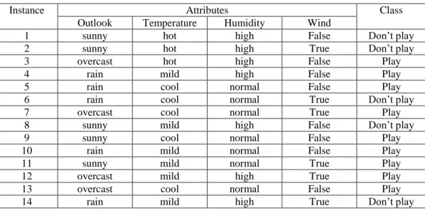
Generally in supervised machine learning application the data correspond to a table of instances; each row representing an instance has an exact number of attributes, along with a class. Commonly attributes are of two types – numeric or nominal. In the Table 2.1 [18] fourteen instances representing different unsuitable and suitable days to play tennis. For each instance there are four features – Humidity, Outlook, Wind and Temperature, with a class label to precise whether or not the day is appropriate to play tennis.
Table 2.1.Tennis dataset
Instance Attributes Class
Outlook Temperature Humidity Wind
1 sunny hot high False Don’t play
2 sunny hot high True Don’t play
3 overcast hot high False Play
4 rain mild high False Play
5 rain cool normal False Play
6 rain cool normal True Don’t play
7 overcast cool normal True Play
8 sunny mild high False Don’t play
9 sunny cool normal False Play
10 rain mild normal False Play
11 sunny mild normal True Play
12 overcast mild high True Play
13 overcast cool normal False Play
14 rain mild high True Don’t play
In a classic machine learning application there are two important data sets such as training sample and testing sample. The training sample is used to learn the concept to the algorithm and the testing set to evaluate the precision of the learning process. During the testing phase, the classes are not presented to the algorithm. The testing set is fed in the algorithm as input, and the algorithm gives as output the class label of each testing instance.
2.3.Learnıng Algorıthms
A learning algorithm is a model that can study and learn or get knowledge from data. Such algorithms proceed by constructing a model based on inputs, and then utilize these inputs to make decisions or predictions, instead of only following expressly programmed instructions.For example, Naive Bayes is a probabilistic summary form of knowledge; C4.5 [19]is a decision tree form of knowledge.
In this thesis, four machine learning algorithms are utilizedfor the comparison of the effects of attribute selectors on the data. These are ANN, naive Bayes, K-NN
and C4.5 − each one of them hasa disparate learning method. These learning algorithms are commonly utilized by researchers, because they have shown their efficiency. ANN and C4.5 are the most developed algorithms of the four. The result of C4.5 algorithm is represented by a decision tree and is easy to interpret. Naive Bayes and K-NN are popular in the community because they are easily implementable and could perform as well as the sophisticated algorithms. [20-22]. The four following sections briefly present these algorithms.
2.3.1. Naive bayes
This algorithm is a kind of reduced form of Bayes approach used to evaluatewhether or not a new instance belongs to a class. The attribute values of the instance is utilized to calculate the posterior probability of classes; if the posterior probability of an instance according to a class is the highest then this instance appertain to this class. In Naïve Bayes, from a statistical point of view the attribute are independent according to each class (Equation 2.1).
𝑝(𝐶
𝑖|𝑣
1, 𝑣
2, … , 𝑣
𝑛) =
p(𝐶𝑖) ∏ 𝑝(𝑣𝑗|𝐶𝑖) 𝑛𝑗=1
p(𝑣1,𝑣2,…,𝑣𝑛) (2.1)
In the equation 2.1, the left side represents the posterior probability of the class label
Ciaccording to the attribute values
< 𝑣
1, 𝑣
2, … , 𝑣
𝑛>
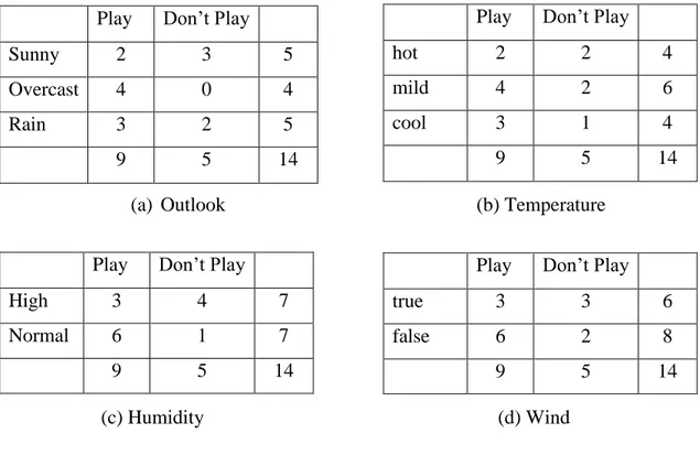
present in the instance. The bottom part of the right side could be excluded because it is a constant and the same for all attributes regarding the class.In the Table 2.2, the sub-tables a, b, c and d are eventuality tables representing the distribution frequency and the correlation between classes andattributes in the tennis data. These sub-tables are important for the calculation of the necessary probabilities to implement Equation 2.1. Now let make an example, image that someone at a certain moment in the journey want to know whether yes or
not the weather is favourable to play tennis. Whereas the outlook is rain, the temperature is cool,
Table 2.2. Correlation between features and classes of the tennis data
Play Don’t Play
Sunny 2 3 5
Overcast 4 0 4
Rain 3 2 5
9 5 14
Play Don’t Play
High 3 4 7
Normal 6 1 7
9 5 14
the humidity is high and the wind is false (there is no wind). We use the Equation 2.1 for the calculation of the posterior probability of each class, utilizing the information in the sub-tables a, b, c and d of the table 2.2:
Play Don’t Play
hot 2 2 4
mild 4 2 6
cool 3 1 4
9 5 14
Play Don’t Play
true 3 3 6
false 6 2 8
9 5 14
(a) Outlook (b) Temperature
Here the posterior probability of the class “Play” is high than the posterior probability of “Don’t Play”, therefore on this day we could play tennis.
Moreover because in naïve Bayes the attributes values are autonomous in the class, the performance prediction can be negatively influenced by the attendance of redundant attributes in the data especially in the training data. In 1994 Sage and Langley found that the performance of naïve Bayes ameliorates when redundant attributes are removed [22]. But, Pazzani and Domigos discovered that even if strong dependencies between the attributes negatively influenced the performance, when average correlations exist between the features naïve Bayes can still well perform [23].
2.3.2. C4.5 decision tree
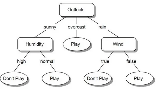
The algorithms ID3 [24] and his successor C4.5 [19], represent in a kind of decision tree representing the training result. In practice decision tree algorithm is popular in the community, this is due to the fact that decision tree algorithm is fast in execution, robust and also because it produce a clear concept description, which is easily interpretable by the users. The Figure 2.2 presents a decision tree representing the tennis data’s training result.The features are represented as nodes in the tree, their associated or domains values as branches and the leaves on bottom represent the classes. Therefore to determine the class of a new instance, one first considers the values of the instance's attributes in the tree and then follows the corresponding values of the branches until reaching the leaf that indicate the class of the attribute.
Fig. 2.2.Tennis data decision tree. Nodes correspond to attributes; the branches are the attributes’
values and the leaves represent the classes.
In ID3 and C4.5 a greedy approach is used to form a decision tree. To select a feature as the root in ID3, one calculates first the entropy.
𝐸𝑛𝑡𝑟𝑜𝑝𝑦(𝑆) = ∑ −𝑝𝑖𝑙𝑜𝑔2𝑝𝑖 𝑐
𝑖=1
(2.2)
In the equation 2.2, the left side of the equation represents the entropy of the whole dataset S, and 𝑝𝑖is the portion of Sbelonging to classi; the logarithm is in base 2 because entropy is a measure of the expected encoding length measured in bits.Then we calculate the Gain (S,A) representing the information gain of each feature, defined as:
𝐺𝑎𝑖𝑛(𝑆, 𝐴) = 𝐸𝑛𝑡𝑟𝑜𝑝𝑦(𝑆) − ∑ |𝑆𝑣|
|𝑆| 𝐸𝑛𝑡𝑟𝑜𝑝𝑦(𝑆𝑣) 𝑣∈𝑉𝑎𝑙𝑢𝑒𝑠(𝐴)
Where Ais an attribute with a possible set of values, and 𝑆𝑣 is a subset of 𝑆for which the attribute 𝐴 has the value 𝑣.After this the feature which has the best information gain value becomes the root of the tree.To do the same thing (choose the root of the decision tree) C4.5 utilized the criterion of gain ratio[24] to determinate the feature that will be at the root of the decision tree. It chooses among the features with a good information gain,the one that optimizes the result of the division of its gain ratioby its entropy; the algorithm is iteratively repeated to create sub-trees.
In the community C4.5 is used as a benchmark algorithm against which the others learning algorithms performance is compared. C4.5 algorithm is fast, robust, accurate and above all it produces a structural comprehensible decision tree. Moreover, it deals very well with redundant and irrelevant data, That is why the influence of data reduction on its accuracy is little[25]. Even so, the decision tree’s size can be reduce after removing redundant and irrelevant data[25, 26].
2.3.3. K-Nearest neighbours
K-NN[8] is an instance based learner but sometimes it is also call a lazy learner because it postpones the learning to the classification moment not before, and its power is in the instances matching plan. In K-NN algorithm, the learning is represented in the form of experiences or specific cases. It is based on effective approximation methods that recover the previous stored cases in order to know the class of a new pattern. K-NN as Naive Bayes generally consists of simple computations [27].
In K-NN to classify a new instance, the closest stored instance to the instance to be classified is determined using the Euclidean distance metric, then the class of this closest one is assigned the new instance.Euclidian distance formula is given as;
𝐷(𝑥, 𝑦) = √∑ 𝑓(𝑥𝑖, 𝑦𝑖) 𝑛
𝑖=1
This equation determines the Euclidean distance𝐷 betweenxandytwo instances; 𝑥𝑖and 𝑦𝑖refer to the 𝑖𝑡ℎ attribute value of patternx and y and for numeric pattern value 𝑓(𝑥𝑖, 𝑦𝑖) = (𝑥𝑖− 𝑦𝑖)2.
K-NN can deal with irrelevant data, but to do so it need more training data, as a matter of fact, to maintain or reach a certain accuracy level, it has been demonstrated that the number of training datamust increase exponentially with the irrelevant data’s number [2, 28, 29].
For this reason, after removing from the training cases noisy and redundant data it is possible to ameliorate the accuracy of nearest neighbour even if the remaining training data is restricted.
Moreover, because each instance to be classified should be compared successively to each stored training instance, the execution takes a lot of time. But the speed of the algorithm can be improved after reducing the training data’s number
2.3.4. Artificial neural networks(ANN)
An ANN is a computer model that combines the human intelligent and the computers processing power; thereby it is able to process a large amount of data simultaneously from experience it has acquired[30]. ANN has several qualities that make them suitable for medical data processing. They are able to extract valuable knowledge from complexes data, something that would be complicated for humans to do [31]. They can also often overcome ambiguous and missing data [32] and provide accurate predications [33]
The most used neural network algorithm is the Multi-Layer Perceptron. A MLP is a set of neurons grouped into different layers these are – input layer, hidden layer(s), and output layer; they form parallel processing units.
The figure 2.3 presents a typical illustration of a MLP, each neuron in a layer is linked to each neuron of the next layer, and the connections are oriented from the
input to the output layer. Then on each connection between two neurons of different layers there is a weight (numerical value) which represents the strength of the connection between these neurones − wij=connection weight between unitsiand j
[34].
In MLP during the training, the connection weights change at each iteration. During the training, when a pattern is presented to the network, computations are done from the input to the output layer then the obtained result is compare to the desired output which is the class label of this pattern; this action is done until the desired iterations number or the stop criterion is reached. This kind of neural network is called a supervised because a desired output is needed in order for it to learn [35].
Fig.2.3.General architecture of MLP
The computation step of feedforward backpropagationmodel neural network proceeds like follow:
(1)
The input layer neurones are activated when the input patterns are put in, this introduces the feedforward process(2)
The outputs of the first layer’s neurones become the inputs of the next layer’s neurones, we call it net input,𝑁𝑗 = ∑ 𝑤𝑗𝑘 𝑜𝑘 𝑃
𝑘=1
(2.5)
Where 𝑜𝑘= output from previous units going on the next unit jas input, then 𝑃= number of inputson unit j.
(b)
The value of their activation function is calculating with their net input:𝑎𝑗 = 𝐹𝑗(𝑁𝑗) (2.6)
The activation function𝐹𝑗is generally a sigmoid function: 𝐹𝑗 =
1
1 + 𝑒−(𝑁𝑗−𝜃𝑗) (2.7)
(3)
Again the units’ outputs of this layer become the net inputs for the next layer. This process continues until it reaches the output layer, then the activation values of the output layer are called the actual output of the neural network computation.Like explained by Rumelhart[36],the adjustment of the weights connections in the generalized delta rule is performin a given training case through the gradient descent on the total error:
∆𝑤𝑖𝑗 = 𝜂𝛿𝑗𝑜𝑗 (2.8)
In this formula, η refers to the learning rate which is a constant; δj= the
gradient error of the net input at unitj. δjis found by the subtraction of the computer activations aj (also called actual outputs)from the expected activations tj (also called desired outputs):
𝛿𝑗 = (𝑡𝑗− 𝑎𝑗)𝐹′(𝑁
𝑗) (2.9)
whereF’ refers to the activation function’s derivative. At the hidden layer, the desired outputs are not known. The next equationrefers to the gradient error givesδj
formulafor the hidden layers:
𝛿𝑗 = (∑ 𝛿𝑘𝑤𝑗𝑘 𝑃
𝑘=1
) 𝐹′(𝑁𝑗) (2.10)
In the equation (2.10), a layer, the error rating to a hidden unit relies on the error of the units that affect it. Furthermore, the connection’s weight between the hidden unit and the units that affect it influence the error’s amount that coming from these units. The disadvantage of this algorithm is that it does not guarantee convergence toward a local minimum.
2.4.Performance Assessment
In a learning task, one of the most important steps is the performance assessment of the learning algorithms. Moreover, it is not just crucial for comparison of different algorithm, but it is an entire part learning algorithm.Although many others criterion of machine learning algorithms performances evaluation have been proposed; the testing set classification precision is the most used criterion[37, 38].
In this work, testing data classification precision is the main assessment criterion for all experiments; different data reduction methods and machine learning algorithms are utilized. A Data reduction algorithm is effective when the data amount is reduced and in addition the learning algorithm accuracy remains the same or improves. The classification precision is determined as the percentage of the training set elements properly classified by the algorithm. The error rate is therefore defined by − one minus the testing set accuracy. Utilizing the test set accuracy to measure the precision of the algorithm is better than utilizing the training instances because they
have already been utilized to induce or create concept description. However sometimes the data is limited, in this case it is important to resample the data by partitioning it into two sets like usual – training and test sets. Then the machine is trained and tested with each set and the final accuracy is the average of both (training and testing) sets accuracies.
2.5.Weka Toolbox
In data mining, experiences have demonstrated that no single learning algorithm is suitable for all cases in data mining. In the real world, datasets vary, and for a machine learning algorithm fits with a dataset and gives and accurate model, the bias of this machine learning algorithm must accommodate the domain structure of the data. Therefore the universal learning algorithm is an utopia[7].
The workbench of Weka is a data processing tools and machine learning algorithms collection. It is shape so that we could easily experiment or test on a new dataset existing data mining methods in flexible ways.It affords almost all the tools for the whole experimental process of data mining, encompassing input data preparation, statistical evaluation of learning models and the visualization of the input samples and the learning result. It also provides a large variety of preprocessing tools. All those detailed and complete toolkit is available on one interface so that the users can easily compare different methods then choose among them the suitable one or the most accurate for the problem he want to solve.
Weka stands for Waikato Environment for Knowledge Analysis. It was developed in New Zealand at the University of Waikato. It has been written with the java programing language and published under the terms of the GNU General Public Licence. Furthermore, Weka can be used on practically any platform. It provides the same interface for most of the learning algorithms, together with techniques for pre-processing and post-pre-processing and for the evaluation of learning algorithms on any given dataset.The Wekaworkspace consist of methods for almost all the standard data mining issues − clustering, regression, association rule mining, data reduction, and classification. The data is represented in a relational table, the formats which can
be read are varied these are: ARFF, XLS, CSV, XLSX, etc.Weka provides implementations of learning algorithms that you can easily apply to your dataset. It also includes a variety of tools for transforming datasets, such as the algorithms for discretization. You can pre-process a dataset, feed it into a learning scheme, and analyse the resulting classifier and its performance−all without writing any program code at all.
One important way of utilizing Weka is to apply on a dataset a learning algorithm and analyse the output result to learn something about the data. Moreover it could be beneficial to use different learning algorithms to process a dataset them compare the results and choose the best one for prediction. In Weka the learning methods are called classifiers and tools for preprocessing are called filters.
3. FEATURE SUBSET SELECTION
To have successful machine learning task, it is important to take into consideration many factors and among them, the most significant is the quality of the dataset. In Theory, having many features should result in a best discriminability, yet, practically it has not always been the case; sometimes, good discrimination (classification) is achieved with limited dataset.
Because of this, the estimation of several probabilistic parameters is not easy. Therefore in order to prevent the training samples overfitting the bias of Occam’s Razor [39]is utilized to construct a simple model that is able to achieve good performance with training sample. This bias sometimes encourage algorithm to favour data with small amount of features than the large ones, and if utilised properly can be fully accurate with the class label; but if the data contains noisy, irrelevant, unreliable or irrelevant data, it becomes difficult to learn throughout the training.
Feature Selection is a process that consists of identifying redundant and irrelevant data and then removes them; this process helps reduce the dimensionality and at the same time allow a fast and effective machine learning task. Moreover, in some cases, the future test performance can be better; in other words, the outcome is more compact and easily interpretable.
Many researches have shown that ordinary machine learning algorithms are negatively influenced by redundant and irrelevant data. Event the K-Nearest Neighbour learning algorithm is sensible to redundant and irrelevant features; its data complexity increases exponentially with the amount of irrelevant features [2, 22, 28]. For decision tree also in some cases such as parity concept, the data complexity can increase exponentially as well. In decision tree algorithm such as C4.5, the training samples can overfit often, having as a result a large tree[26].Therefore, by removing noisy data, in many cases the result can be better resulting in small tree easy to interpret. In Naïve Bayes algorithm, due to the fact that its features are independent in the class, it is also sensitive to irrelevant attributes [22].
In this chapter, we begin in section 3.1 and section 3.2 by reviewing common approaches to attribute subset selection (filters and wrappers) for machine learning
present in literature. In sections 3.3 and 3.4, major aspects of feature subsetselection algorithms and some familiar searching methods (heuristic search)are presented.
3.1. Pattern Recognıtıon And Feature Selectıon
For the last decades, many researches in pattern recognition have been focus on feature selection techniques [40]. Just as for pattern recognition, feature selection is important for machine learning, because they share the same task of classification. In fact the feature subset selection have been developed to facilitate the knowledge extraction from big amount of data, and also to improve its comprehensibility [26]. For example in pattern recognition and machine learning, attribute selection techniques can help economise time in data acquisition, ameliorate precision of classification and ease the perplexity of the classifier [9]. Matter of fact, machine learning is based on both statistics and pattern recognition[4].
3.2.Feature Selectıon Algorıthms
In feature selection, the search is done through a feature space, therefore in order to perform well; it should follow four important steps that positively influence the search[41]:
1. Start step. There are two different way to start the search. The first way is to start with no feature in the space then successively add features. This way of search is called forward search process. Inversely, the search can start with all attributes in the search space and then successively remove the attributes until the best subset remains; this kind of search is commonly called backward feature search. Another way consists to start somewhere in the middle and remove useless attributes from this point.
2. Second step. It is about the search organisation; a complete search of the feature space is not recommended. Because for N initial number of features,
there are 2N possible feature subsets. That is why a heuristic search is better and more conceivable than complete one by one search. Moreover heuristic search can produce good feature subsets, although it cannot every time give or guarantee the optimal subset.
3. Third step. It is about the strategy of evaluation; the only thing that differentiates the feature subset selection algorithm is the way the subsets are evaluated by each algorithm for machine learning. One model called the filter [6, 26] works independently of any machine learning algorithms—before the learning starts, irrelevant attributes are removed from the data. These algorithms are based on heuristics search to decide the quality of attribute subsets using the characteristics or properties of the data. However, some researchers think that the bias of a given learning algorithmshould be taken into consideration for the feature selection. this model is called the wrapper [6, 26], using learning algorithm along with cross validation to approximate the precision of the subsets of feature. An illustration of both models wrapper and filter is shown in Fig.3.1
4. The Fourth step is about stopping criterion; it is crucial for the feature selection algorithm to determine when to end the searching in the feature subsets space. According to the assessment strategy, a feature selection algorithm has to stop removing or adding attributes when none of the remaining attributes ameliorates the worth of the existent subset of feature. Otherwise, the feature selector could continue to correct the subset as the quality of the subset does not decrease.
Fig.3.1. Wrapper and Filter algorithms [4]
3.3.Heurıstıc Search
When a feature selector is dealing with a large amount of features to extract the best feature subset from a feature subsets space and we want it to be done in an acceptable time, it is important to define constraints. For example, the greedy hill climbing, an ordinary search method provides local adjustment to the current subset of feature. Frequently, the local adjustment is merely the deletion or the addition of a single attribute to the subset.
In a feature selection algorithm, when only deletions from the feature subset is considered it is called a backward elimination; but when it only considers additions it is called forward selection[3]. Alternatively a method called stepwise
get the subset of features, in the algorithm pay attention to every variation in the feature subset then opt for the best, or in some case may merely select the feature subset that first ameliorate the worth of the current subset.In both case, when a change is admitted, it is never reconsidered. Fig.3.2 presents the feature subset space for tennis dataset. If swept from the bottom to the top the figure presents all possible local deletion; if scanned from the top to the bottom, it presents all the addition to each node [4].
Fig.3.2. Space of feature subset for the “tennis” dataset [4]
The Table 3.1 presents the greedy hill climbing search algorithm.The Best first search [42] is an Artificial Intelligence method that permits backtracking on the search way. The best first goes through the feature subset search space just like greedy hill climbing algorithm by making local modification to the current subset of feature.
Table.3.1. Algorithm of Greedy hill climbing search [73]
1. Let s ← start state.
2. Expands by making each possible local change. 3. Evaluate each child t of s.
4. Let s’ ← child t with highest evaluation e(t). 5. If (s’) ≥ e(s) then s←s’, goto 2.
Yet, differently to hill climbing algorithm, if the explored path performance begins to decrease, the best first algorithm may backtrack to another encouraging previous subset and from there continue the search. In the best first search, it is important to define a stopping criterion otherwise the search will go on until the exploration of entire space and this can take enough time. Table3.2 describes the algorithm of the best first search.
Table 3.2.The Best first search algorithm [72]
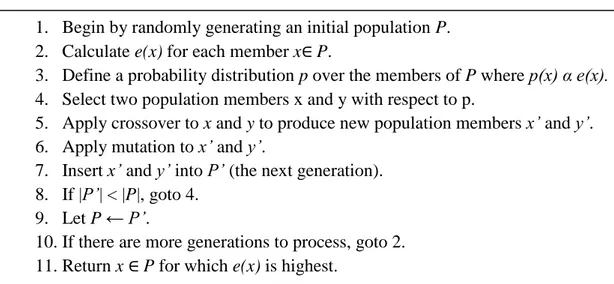
Genetic algorithms are adaptive search methods founded on the criterion of natural biological selection [12]. They utilize many rival solutions—changed over time—to move toward a best solution.
In fact, to help keeping off local optima the space of solution is searched in parallel. For attribute selection generally, a result is a fixed (determined) binary length of string corresponding to a subset of feature—each value location in the string corresponds to the absence or presence of an individual feature. The algorithm is an iterative process in which each consecutive generation is created by using genetic operators such as mutation and crossover to the current generation members. Crossover put together different features from a couple of subsets in a new subset.While mutation transforms some of the values (thereby deleting or adding features) in a subset arbitrarily. The genetic operators’ utilization on population members is defined by their fitness (quality of a subset of feature compared to an evaluation strategy); then through mutation and crossover, the better features subsets
1. Begin with the OPEN list containing the start state, the CLOSED list empty. And Best ← start state.
2. Let s = arg max e(x) (get the state from OPEN with the highest evaluation). 3. Remove s from OPEN and add to CLOSED.
4. If e(s) ≥ e(BEST), then BEST ← s.
5. For each child t of s that is not in the OPEN or CLOSED list, evaluate and add to OPEN.
6. If BEST changed in the last set of expansion, goto 2. 7. Return BEST
have more chance to be selected to become a new subset. A simple genetic search strategy is shows in table3.3. Crossover combines different features from a pair of subsets into a new subset. The application of genetic operators to population members is determined by their fitness (how good a feature subset is with respect to an evaluation strategy). Better feature subsets have a greater chance of being selected to form a new subset through crossover or mutation. In this manner, good subsets are “evolved” over time. Table 3.3 definesalgorithms of a simple genetic search strategy step by step.
Table 3.3. Simple genetic search strategy
3.4.Wrapper Methods For Feature Selectıon
Wrapper methods for feature subset selection are methods that use learning algorithms to justify the quality of subsets of features. The principle of Wrapper approaches is that the induction or learning algorithm which is going to use the subset of feature must provide the best accuracy (Lan94). Often wrappers methods results are better than filter methods. This is due to the fact that in wrapper approaches, a specific learning algorithm and a training data are tuned together, then different subsets of the training data are tested until the best subset according to the induction algorithm is obtained. However compared to filters, wrappers are very
1. Begin by randomly generating an initial population P. 2. Calculate e(x) for each member x∈ P.
3. Define a probability distribution p over the members of P where p(x) α e(x). 4. Select two population members x and y with respect to p.
5. Apply crossover to x and y to produce new population members x’ and y’. 6. Apply mutation to x’ and y’.
7. Insert x’ and y’ into P’ (the next generation). 8. If |P’| < |P|, goto 4.
9. Let P ← P’.
10. If there are more generations to process, goto 2. 11. Return x ∈ P for which e(x) is highest.
slow because they frequently call the learning algorithm and when a different learning algorithm is used, they rerun. This section presents works centred on wrapper methods and techniques to decrease its computational cost.
3.4.1. Wrapper using decision trees algorithms
In 1994, Pfleger and Kohavi[43]have been the first researchers to propose the Wrapper as common technique for feature subset selection; they presented two precise characteristics of attribute relevance and affirmed that wrapper could find relevant attributes in a training set. According to them, given a full feature set, an attribute Xi is hardily relevant if the performance or the accuracy of the class values distribution decrease when it is removed. An attribute Xi is considered as slightly relevant when it is not hardily relevant and the accuracy of the class values distribution given a feature subset S of the full subset decrease when it is removed. However when an attribute is not hardily or slightly relevant it is irrelevant. To demonstrate this, experiments were done on different data utilizing ID3 and C4.5 as learning algorithm. The results demonstrate that feature selection did not importantly improve the accuracy of C4.5 or ID3. The main benefit was the reduction of the tree size.
During the 90's, many researchers tried to improve wrappers methods, among them Shavlik and Cherkauer[16]who in order to ameliorate wrapper on Decision tree algorithms utilized the genetic search approach. This approach successively ameliorates the accuracy of ID3 on a classification task. More precisely, to achieve this, they proposed an algorithm called SET-Gen whose purpose was to improve the accuracy as well as the easy comprehension of decision tree. This algorithm utilizes a fitness function: 𝐹𝑖𝑡𝑛𝑒𝑠𝑠(𝑋) =3 4𝐴 + 1 4(1 − 𝑆 + 𝐹 2 ) (3.1)
whereX represents subset of feature, A is C4.5 cross validation accuracy average, S average of the tree size generates by C4.5 and F the features number in a subset.
3.4.2. Wrapper using naïve bayes classifier
Sage and Langley[22]due to the fact that in Naive Bayes classifier the distribution probability of a given feature is independent from the others, claim that the accuracy of Naive Bayes could be ameliorate if the irrelevant attributes are removed from the training set. In order to choose features that are going to be used with Naive Bayes, a strategy of forward search is utilized, unlike to decision tree learners that generally are used with backward strategy. The reason why forward search strategy is used is because it instantly discerns dependencies when irrelevant features are added. To test this assumption many experiment have been done and the selected features improved the performance during the classification task.
In the concern to ameliorate the precision of Naive Bayes Classifier, Pazzani[14]associates in a wrapper framework a simple constructive induction and feature selection. Then a comparison of backward and forward hill climbing search is done. The experiments results show that both methods ameliorate the Naive Bayes accuracy. Yet the forward search strategy is advantageous than backward search in removing irrelevant features because it begins with all the set of features and takes in consideration all the possible pair of attributes. The backward search strategy is efficient in determining interaction between features.
3.4.3. Wrapper improvement techniques
The computational expense of wrappers techniques is the basis of most of the blame on wrappers. With wrappers, each potential subset of feature is tested in a k-fold cross validation manytimes using a learning algorithm; therefore on a dataset with large amount of feature, the wrapper can be extremely slow. This handicap has pushed many researchers to do some research to find a way to reduce the
computational cost of wrapper approaches. In 1994, a system that stores decision tree has been conceived by Caruanna and Freitag[15]; this to decrease the trees number generate over wrapper feature subset selection and free larger space for searches. In order to reduce the computation time of best first search and backward strategies, John and Kohavi[44]have presented the concept of Compound Operators. In a search of feature subset, the first Compound Operator is constructed after the full backward or forward search evaluation of a given set of features; the creation of the Compound Operator combines the two best subsets. Then this operator is utilized on the feature set to create a new feature subset, and if this subset ameliorates the performance, another operator is created and this time combining the best three subsets, and so on. The Compound Operator is very useful in the search of the best subset of feature. To verify the effectiveness of this technique, the compound operators were used with forward best first search to find a subset of feature, then this subset was trained and test with Naive Bayes and ID3. The results presented no important improvement of the precision for Naive Bayes and ID3. However, combining with backward search, the operators ameliorated the precision of C4.5 but insignificantly degraded the accuracy of ID3. The good result with C4.5 is due to pruning in C4.5 algorithm process which permits the best first search to surmount local minima, which is not the case for ID3.
A technique to compare concurrent feature subset selectors has been introduced in 1994 by Moore and Lee[10]. It is a forward selection algorithm. In this algorithm, a subset is removed from the competition of the best feature subset if over the leave-one-out cross validation this subset is considered to be improbable to have the smallest error rate; moreover the indistinguishable subsets are blocked; only one remains in the competition. This technique has the advantage to decrease the number of subsets that are going to be used over the training; therefore it reduces the computational time of the full evaluation. The competition cease as soon as only one subset of feature remains.
3.5.Filter Methods For Feature Selection
In machine learning, the first approaches concerning the feature selection algorithms were filter techniques. Those techniques are based on heuristic search rather than learning algorithms to assess the worth of feature subsets. As a matter of fact, filter techniques are faster than wrapper techniques; moreover they are simple, more practical and most of the time more effective on high dimensionality data.
3.5.1. Filters through consistency subset
In 1991 Almuallim and Dieterich[11] present the FOCUS algorithm which was originally made for Boolean domains; this algorithm completely searches the feature subset space until it reaches the minimum combination of attribute that shares the training set into pure classes where each combination of attribute values belong to a single class. This is called "min-features bias". After that, the ID3 [24] is used to build the decision tree of the final feature subset. As Freitag and Caruanna [15] have figured out, there are two great issues with FOCUS algorithm. The first one is that sometimes in FOCUS a complete search may be impossible if many attribute are needed to reach consistency. Secondly, an acute bias for consistency may be unwarranted statistically and can drive to an overfitting of the training set; because to solve only one inconsistency, the algorithm will keep adding features.In 1994 Almuallim and Dieterich[45]deal with the first of these issues. Three algorithms were designed to make FOCUS algorithm able to deal computationally with many features. These algorithms were forward selection search combined with heuristic to approximate the "min-feature bias". Thus using the following formula of information theoretic, the first algorithm assesses features:
𝐸𝑛𝑡𝑟𝑜𝑝𝑦(𝑄) = − ∑ 𝑝𝑖+ 𝑛𝑖 |𝑆𝑎𝑚𝑝𝑙𝑒|[ 𝑝𝑖 𝑝𝑖+ 𝑁𝑖 𝑙𝑜𝑔2 𝑝𝑖 𝑝𝑖+ 𝑁𝑖 + 𝑛𝑖 𝑝𝑖+ 𝑛𝑖 𝑙𝑜𝑔2 𝑛𝑖 𝑝𝑖+ 𝑛𝑖 ] 2|𝑄|−1 𝑖=0 (3.2)
where, Q represents a given subset of feature, and there are 2Q possible truth value assignments to the features. The training set instances in a given set of feature Q are divided with equal truth value assignments in Q. In each group, the Equation above calculates the general entropy of the class values; ni and pirespectively represent the negative and positive number of examples in the ith group. At each step, the attribute which minimises the equation is put in the current subset of feature.
In the second algorithm, at each step of the search, the feature that presents the most discriminating characteristics is chosen and added to the current feature subset. A feature is discriminating if for two given examples negative and positive, the value of this feature is different for each one of them. At each step, the chosen feature is the one that discriminates the largest number of negative-positive couples of examples—which have not yet been discriminated by any existent feature in the subset.
The third algorithm looks like the second algorithm excepting the fact that a weight is incremented to the count of each feature that discriminate a negative-positive example pair. This increment relies on the number of feature that differentiates or discriminate the pair.
In 1996 Setiono and Lui[13] present the LVF algorithm comparable to FOCUS algorithm. It is consistency driven but differently to FOCUS, it can deal with irrelevant data if the irrelevant data level is approximately known. The LVF during the successive iteration randomly produces a subset S. İf the feature number of the S is fewer than the feature number of the current best subset, then the inconsistency rate of S and the inconsistency rate of the current best subset are compared and if S is at least as consistent as the best current subset, the best current subset is replaced by S.Setiono and Liu made some experiments with LVF; they used dataset with big amount of features and instances. They have shown that LVF was capable to reduce features number by more than half.
3.5.2. Feature selection by discretization
According to Liu and Setiono [17] it is possible to select feature using discretization methods. Combining Chi2 algorithm and discretization it is possible to create a feature selector. Initially the numerical features are sorted by positioning each attribute value in its interval. Then each attribute is discretized with χ2 test to define when adjacent intervals should be merged. Then, to control the merging operation's extent, they used a χ2
threshold which has been set automatically. This threshold is defined by trying to keep the structure of the original data. The process is ensured by inconsistency which is measured like in LVF algorithm.
Three reports have been done by the authors on data containing both numeric and nominal data utilizing C4.5 [24, 46] before and after discretization. They came to the conclusion that Chi2 is efficient at eliminating some features and improving C4.5 accuracy. However we really don't know whether it is the removing of some features or the discretization that is to the basis of the C4.5 performance improvement.
3.5.3. Feature filter using information theory
In 1996, Sahami and Koller[47]have developed a new feature selection algorithm based on probabilistic reasoning and information Theory[18]. Thereasons behind this feature subset selection method are that as the purpose of machine learning or pattern recognition algorithms is to evaluate the probability distributions for a class value. So the selected feature subset should remain as close as possible to the original distributions. For example consider a set of classes C, a set of features V, a subset X of V, v a set of values (v1,...,vn) assigned to each features, and vx the projection of the values in f onto variables in X. The purpose of feature selection algorithm is to define X so that Pr(C|X=vn) remains as close as possible to
Pr(C|V=v). To do so the algorithm starts with the original features and at each step
or stage, using the backward elimination search, it removes the feature that generates between the two distributions a change. To approximate the difference between two distributions, the cross entropy is utilized, also the number of features to be removed
by the algorithm must be specified. Given two different features, the cross validation of the class distribution is given as:
𝐷(Pr(𝐶|𝑉𝑖 = 𝑣𝑖, 𝑉𝑗 = 𝑣𝑗) , Pr(𝐶|𝑉𝑗 = 𝑣𝑗)) = ∑ 𝑝(𝑐|𝑉𝑖 = 𝑣𝑖, 𝑉𝑗 = 𝑣𝑗)𝑙𝑜𝑔2 𝑝(𝑐|𝑉𝑖 = 𝑣𝑖, 𝑉𝑗 = 𝑣𝑗) 𝑝(𝑐|𝑉𝑗 = 𝑣𝑗) 𝑐∈𝐶 (3.3)
From the remaining features, a set Mi composed of K attributes is found by the algorithm for each featurei, That is supposed to contain information that feature i has about class values. The features present in Mi have been taken from the remaining features for which the value of the Equation 3.3 is smallest. For each feature i, the cross entropy is calculated between the class distribution given only Mi and the class distribution given Mi, Vi. Then after the cross entropy performed for each feature i is done, the feature with the minimal quantity is deleted from the set. This process is executed until the number of features specified by the user is removed from the original dataset.
Experiments have been done on different dataset from different domains using Naive Bayes and C4.5 as learning algorithms. The experiments showed that the results of the feature selection algorithm are good when the size K of the conditioning Set M is set to 2. Also the algorithm is capable to reduce by more than half the features number in two domains having more than 1000 attributes, moreover it ameliorate the performance by about one or two per cent.
The problem of this algorithm is that to be encoded in binary the feature must have more than two values in order to avoid the bias that entropic measures have toward features with many values.
![Table 3.2.The Best first search algorithm [72]](https://thumb-eu.123doks.com/thumbv2/9libnet/4634138.86173/38.892.149.753.384.599/table-the-best-first-search-algorithm.webp)