Identification of breast cancer using the extreme learning machine assisted by firefly algorithm

Sayı 17, S. 637-644, Aralık 2019

© Telif hakkı EJOSAT’a aittir

Araştırma Makalesi

No. 17, pp. 637-644, December 2019

Copyright © 2019 EJOSAT

Research Article

Ateş Böceği Algoritması Destekli Aşırı Öğrenme Makinesi ile Göğüs

Kanseri Veri Kümelerinin Sınıflandırılması

Deniz Üstün

1 _{Karamanoğlu Mehmetbey Üniversitesi, Mühendislik Fakültesi, Bilgisayar Mühendisliği Bölümü, İstanbul, Türkiye (ORCID: 0000-0002-5229-4018)}

(İlk Geliş Tarihi 24 Eylül 2019 ve Kabul Tarihi 5 Kasım 2019) (DOI: 10.31590/ejosat.623816)

ATIF/REFERENCE: Üstün, D. (2019). Ateş Böceği Algoritması Destekli Aşırı Öğrenme Makinesi ile Göğüs Kanseri Veri

Kümelerinin Sınıflandırılması. Avrupa Bilim ve Teknoloji Dergisi, (17), 637-644.

Öz

Göğüs kanseri hastalığı, kadınların ölümüne neden olan ikinci kanser türüdür. Kanser hastalığının erken teşhisi ve kanser hücrelerine uygulanan uygun ve doğru tedavi hastalığın ölümcül riskini azaltabilir. Tıp doktorları, kanser hastalığının teşhisinde zaman, zaman hata yapabilmektedirler. Yapay zeka tekniklerinin (YZT) performansı, bilgisayar donanım teknolojilerindeki hızlı gelişmeler sayesinde artmıştır. Buna bağlı olarak, kanser hastalığının tanı doğruluğunun arttırılması ile ilgili olarak YZT’ler kullanılabilir. Standart Eğime Dayalı Geri Yayılım Yapay Sinir Ağları (GY–YZT), göğüs kanseri hastalığının tanısında yaygın olarak kullanılmaktadır. GY–YZT, kanser hastalığının teşhisinde iyi bir performans sergilese de, yerel minimum ve eğitim sürecinde uzun süre takılma gibi bazı sınırlamaları vardır. Bu çalışmada, Göğüs Kanseri Wisconsin veri kümesinde göğüs kanseri hastalığının teşhisi için, sezgisel ateş böceği algoritması tarafından desteklenen aşırı öğrenme makinesi (AB–AÖM) önerilmiştir. Önerilen AB–AÖM’nin hastalık tanı üzerindeki performansı standart AÖM ve GY–ANN yöntemleriyle karşılaştırıldı. Sonuçlar, AB–AÖM’nin sınıflandırma performansıyla ilgili anlamlı bir gelişme sağladığını ve tıbbi problemler için güçlü bir teknik olarak kullanılabileceğini göstermektedir.

Anahtar Kelimeler: Aşırı öğrenme makineleri, ateş böceği algoritması, göğüs kanseri, tıbbi karar destek sistemleri.

Identification of Breast Cancer Using the Extreme Learning Machine

Assisted by Firefly Algorithm

Abstract

The Breast cancer is the second cancer type which causes death of women. The premature detection of cancer and the suitable treatment applied to cancer cells can reduce the deadly risk. The medical doctors can make faults in diagnosis of the cancer disease. The performance of artificial intelligence methods (AIMs) containing increased thanks to rapid improvements in the technologies of the computer hardware. AIMs can be used regarding the enhancement of diagnostic accuracy. Standard Gradient–Based back propagation artificial neural networks (BP–ANN) has been commonly utilized in the diagnosis of the breast cancer disease. Even though BP–ANN are good performance in the diagnosis of cancer disease, it has some limitations such as possible to be trapped in local minima and long time in the training process. In this study, the extreme learning machine assisted by heuristic firefly algorithm (FF–ELM) is proposed for diagnoses of breast cancer disease on the Breast Cancer Wisconsin Dataset. The diagnostic performance of proposed FF–ELM was compared with the standard ELM and BP–ANN methods. The results show that FF–ELM provides a meaningful enhancement regarding the classification performance and it can be used as a powerful technique for the medical problems.

Keywords: Extreme learning machines, firefly algorithm, breast cancer, medical decision support systems.

* _{Sorumlu Yazar: Karamanoğlu Mehmetbey Üniversitesi, Mühendislik Fakültesi, Bilgisayar Mühendisliği Bölümü, İstanbul, Türkiye, ORCID:}

1. Introduction

The uncontrolled cell division in an organ causes the tumors that can be cancerous. There are two sorts of tumors as the malignant and benign. The malignant that is cancerous tumor is growing, spreading out and menacing of life. On the other hand, benign or non– cancerous tumor is not spreading and not threatening of life [1]. If the uncontrolled growing cells are in the tissue of the breast, it is defined as the malignant breast cancer. In general, breast cancer disease the second cancer type which causes death of women [2]. Early diagnosis of the breast cancer disease and then the appropriate treats applied to cancerous cells can decrease the deadly risk for the humans with cancer disease. Therefore, the detection of malignant and benign for the cell with tumor depending on the classification features is very important [3]. The truth diagnosis in the early detection of cells with tumor has been proven to decrease the death rate caused by the disease of the breast cancer [4]. Sometimes the medical doctors depending on capability of expertise in the detection of tumor sort can mistake in the diagnosis of the cancer disease. While the diagnosis with an accuracy rate of 79.9% made by an expert medical doctor, the artificial intelligence methods containing the machine learning and data mining is achieved the accuracy rate of 91.1% [5]. Identification and classification technologies which are a large part of machine learning based on artificial intelligence have gained an increasing interest in biomedical science area through its skill extracting complicated relationships between input and output parameters in big datasets stored related to the biomedical science. Recent researches focus on subjects such as the treatment processes of human diseases, understanding the structure of biological systems, improving new drug discovery targets and giving insights for diagnostic methods.

Artificial neural networks (ANNs) widely used in the regression and classification problems one of best the artificial intelligence methods. The structure of the ANNs is developed by getting inspired the biological neural networks [6]. An ANN structure consisted of three layers that are an input layer, the hidden layers and an output layer. The neurons are located in each layer and they are connected to each other by the weight value updated iteratively until target values. The adjustment of weights is named as training phase and ANN structure is then tested [7]. Many researches illustrate that ANNs achieved good classification performances in the breast cancer disease. However, the methods based on ANNs have some limitations. There are several parameters like the learning rates, the number of hidden layers and the node number of layers and the activation function in the beginning of the ANN training phase. Besides, the training process has taken longer time because of the complex network structure in each iteration requiring the expensive calculation cost and the ANN can trapped in local minima that causes lower performance.

In addition to the alternative learning algorithms, the extreme learning machines (ELMs) which used to train single hidden layer feedforward neural networks (FFNN) recently have been proposed. The starting of the hidden nodes is done randomly and fixed without iterative tuning. Moreover, the hidden nodes of the ELMs do not require to be same neuron. The weight values (free parameters) that have to calculate is the connections among to input, hidden and output layers. As such, ELMs are improved as a model that are interested in the solution of a linear system. In contradistinction for the conventional FFNN learning techniques, ELMs have a greater tendency that achieves a global optimum and they are more efficient [8–10]. ELMs together with the commonly used activation functions can achieve results close to the optimal generalization bound of the conventional FFNN [11]. The generalization and efficiency performance of ELMs compared with the traditional FFNN algorithms have been investigated for a wide range of different problems from the several fields [10, 12]. ELMs have been illustrated for having more efficiency compared with the least square support vector machines (LS-SVMs) [13], standard support vector machine (SVM) [14] and others. However, the ELMs has some limitations such as determination of node number in the hidden layer and selection of activation functions.

In the literature, there are many studies which the diagnosis of cancer is trying to be estimated by ANNs. Moreover, ANNs were combined with other heuristic methods to increase their effectiveness. The clinical reports were given that the ANN was implemented to diagnose breast cancer by using many several features of ANNs [15, 16]. The decision support system is developed on the breast cancer dataset by using an approach combined with probabilistic neural networks and rough sets [17, 18]. Hsiao et al. [19] performed an MLP classifier training using vascular indices (harmonic and non-harmonic 3D power Doppler imaging) to determine whether breast tumors were benign or malignant. In order to contribute the premature diagnosis of breast cancer disease, an artificial neural network is proposed and its accuracy rate is 77% [20]. In another study, The extreme learning method is applied to the breast cancer Wisconsin dataset for diagnosing breast cancer disease [21].

In this study, a method based on the extreme machine learning assisted by firefly algorithm (FF-ELM) is proposed for diagnosing (classification) the breast cancer disease. The FF-ELM is well trained and tested on the Breast Cancer Wisconsin dataset taken from UCI Machine Learning Repository. In terms of the accuracy rate, the performance of FF–ELM are compared with the back propagation artificial neural network (BP-ANN) and standard extreme learning method (ELM). The FF-ELM detects the diagnosis breast cancer with the best accuracy rate of 0.976 as compared with the accuracy rate of 0.964 and 0.921 reached by the ELM and BP-ANN methods, respectively [21]. The obtained results therefore show that the FF-ELM is more accurate than the BP-ANN and standard ELM model for diagnosing of the breast cancer disease.

2. Material and Method

2.1. Breast Cancer Wisconsin Dataset

The FF–ELM is used the Breast Cancer Wisconsin Dataset taken from UCI Machine Learning Repository. The dataset is produced by Dr. William H. Wolberg from the University of Wisconsin Hospital in the Madison [22]. There are two classes that are as the malignant and benign. The dataset consists of 699 samples, 10 attributes and a class property. Amount 65.6% (458 instances) of the

class instances are distributed as benign, the remaining of 34.5% (241 instances) is also dispersed as malignant. The information about attributes is given in Table 1.

Table 1. The information of the attributes for Breast Cancer Wisconsin Dataset [22]

Attributes Value of range

1 Sample code number Id number

2 Clump Thickness 1–10

3 Uniformity of Cell Size 1–10 4 Uniformity of Cell Shape 1–10

5 Marginal Adhesion 1–10

6 Single Epithelial Cell Size 1–10

7 Bare Nuclei 1–10

8 Bland Chromatin 1–10

9 Normal Nucleoli 1–10

10 Mitoses 1–10

11 Class 2: benign – 4: malignant

A preprocessing was applied to the raw data in the dataset to produce well and suitable data for using the training and test steps of the proposed FF–ELM method. Firstly, it was removed the sample code number attribute that is not related to the diagnosis in the dataset. A normalization process that is to be between -1 and 1 was then applied to the remaining nine attributes and it is used as a predictor. Finally, the last attribute was transformed among to 0 (benign) and 1 (malignant) values.

2.2. Standard Extreme Learning Machines (ELMs)

The original ELM method [10] has been proposed by Huang et al for training the single-hidden layer feedforward neural networks (SLFN). The main aim of the ELM algorithm is established on the weights of the hidden layer. Moreover, the bias values randomly produced and the computation of the output weights is performed by utilizing the least squares solution method. The architecture of the ELM is given in Fig. 1.

Fig. 1. The architecture of the standard ELM [10]

where, K represents to a set of unique samples (Xi, ti), where Xi=[xi1, xi2,…, xik]T∈Rk and ti=[ti1, ti2,…, til]T∈Rl. N refers the hidden layer nodes. g(x) is the activation function, which is also a mathematical model that is represented by the following equation.

∑ 𝛽𝑖𝑔𝑖(𝑥𝑗) = ∑ 𝛽𝑖𝑔𝑖(𝑊𝑖𝑋𝑗+ 𝑏𝑖) 𝑁 𝑖=1 𝑁 𝑖=1 (1)

where, J=1, …, K and Wi=[Wi1, Wi2… Wik]T refers the weight vector that connects the hidden node and the ith input nodes. 𝛽�𝑖�=[𝛽�𝑖�1,

𝛽�𝑖�2,……, 𝛽�𝑖�l]T represents the weight vector that connects the hidden node and the ith output nodes. bi represents the ith hidden node’s threshold. Wi .Xj represents the inner product of Wi and Xj. Selection of the output nodes is linearly done, however. The standard of SLFNs and N hidden nodes in the activation function g(x) can be taken as samples of K without error. In other words, mean:∑N𝑗�=1||𝑜�𝑗�−𝑡�𝑗�||=0, i.e., and there exist 𝛽�𝑖�,Wi, and bi in such a way that

∑ 𝛽𝑖𝑔𝑖(𝑊𝑖𝑋𝑗+ 𝑏𝑖) 𝑁

𝑖=1

= 𝑡𝑗, 𝑗 = 1, … , 𝐾 (2)

From the equations given above for K, it can then be presented as follows

where, 𝐻(𝑊1⋯ 𝑊𝑁, 𝑏1⋯ 𝑏𝑁, 𝑋1⋯ 𝑋𝐾) = [ 𝑔(𝑊1𝑋1+ 𝑏1)����⋯ ������𝑔(𝑊𝑁𝑋1+ 𝑏𝑁) ���������⋮ ��������������� ⋯ �������������������� ⋮�������� 𝑔(𝑊1𝑋𝐾+ 𝑏1)����⋯ ������𝑔(𝑊𝑁𝑋𝐾+ 𝑏𝑁) ] (4) 𝛽 = [ 𝛽1𝑇 ⋮ 𝛽𝑁𝑇 ] 𝑁∗𝑙 ������𝑇 = [ 𝑡1𝑇 ⋮ 𝑡𝐾𝑇 ] 𝐾∗𝑙 (5) Eq. 3 is transformed into a linear system. Moreover, the weights of output can be calculated analytically by a least square solution.

𝛽 = 𝐻ⴕ_{𝑇 (6)}

where, 𝐻�† is referred the Moore–Penrose as the inverse matrix for H. Thus, the weights of the output are computed by a mathematical transformation. In this way, the learning parameters such as the iteration number and the learning rate, which affects the training time length of the networks are lifted.

2.3. Firefly Algorithm

The firefly algorithm (FFA) inspiring by the social flashing behavior of fireflies is an optimization method based on a swarm intelligence. An important benefit of the FFA is mainly utilized the randomly generated real numbers and it is carried out the optimization process by using the global intercommunication between of individuals in the firefly swarm. In the firefly algorithm proposed by Xin-She Yang at Cambridge University, the results of the objective function for a given optimization problem are improved by using differences in light intensity. In order to achieve the optimal solutions, the abilities of fireflies moving towards brighter and more attractive locations are used. All fireflies are symbolized by their light intensities related to the objective function given for the optimization problem. The position of each firefly in the solution space is iteratively changed. There are three rules in the firefly algorithm [23–25].

 The gender of all fireflies is unisex and they move towards ones having more attractive and brighter light.

 A firefly attractiveness is commensurate with its brightness that makes smaller as the distance from the other firefly increases. If there is not more attractive firefly than a particular firefly, it will randomly perform the motion.

 A firefly brightness is established by the objective function value. For the maximization problems, the brightness is commensurate with the objective function value.

The attractiveness of each firefly is described by the β symbol and its value is achieved by the monotonically reducing function of the distance (r) among to any two fireflies [23].

𝛽(𝑟) = 𝛽0𝑒−𝛾𝑟 𝑚

, m ≥ 1 (7)

where β0 indicates the maximum attractiveness (at r = 0) and γ is the light absorption coefficient, that controls the reduction of the light intensity. The distance among to two fireflies i and j at positions xi and xj is given as follows [23];

𝑟𝑖𝑗 = ‖𝑥𝑖− 𝑥𝑗‖ = √∑ (𝑥𝑖𝑘− 𝑥𝑗𝑘) 2 𝑑

𝑘=1

(8) where xi,k is the k-th component of the spatial coordinates xi of i-th firefly and d indicates the number of dimensions. The motion of a firefly i is determined by the following form [23];

𝑥𝑖= 𝑥𝑖+ 𝛽0𝑒−𝛾𝑟𝑖𝑗 2

(𝑥𝑗− 𝑥𝑖) + 𝛼 (𝑟𝑎𝑛𝑑 −

1

2) (9)

here, the first term indicates the current position of a firefly i, the other term represents the attractiveness of a firefly. If there are not any brighter firefly, the last term is utilized for the random motion. In the most cases, α ∈ (0, 1) and β0 = 1. The value of the light absorption coefficient (γ) is varied from 0.1 to 10 and this value defines the attractiveness variation and the value is in charge of the FA convergence speed [23]. The individuals in the initial population are produced by using the following expression;

𝑥𝑖= 𝑟𝑎𝑛𝑑(𝑈𝐵 − 𝐿𝐵) + 𝐿𝐵 (10)

where, UB and LB indicate the upper and lower bounds of the i-th firefly. In the algorithm, after the initial population is evaluated, the main loop runs until the fact that the generation (iteration) number reaches the maximum value. In the end of each iteration, the firefly with the maximum light intensity is selected as the possible optimal solution.

2.4. The Performance Metrics

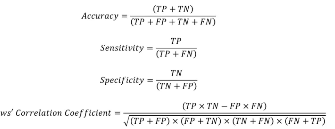
For evaluating the prediction performance of the methods, four quantifying metrics that are accuracy, sensitivity, specificity and Matthews’ correlation coefficient are used [26]. These indices are defined by the following equations;

𝐴𝑐𝑐𝑢𝑟𝑎𝑐𝑦 = (𝑇𝑃 + 𝑇𝑁) (𝑇𝑃 + 𝐹𝑃 + 𝑇𝑁 + 𝐹𝑁) (11) 𝑆𝑒𝑛𝑠𝑖𝑡𝑖𝑣𝑖𝑡𝑦 = 𝑇𝑃 (𝑇𝑃 + 𝐹𝑁) (12) 𝑆𝑝𝑒𝑐𝑖𝑓𝑖𝑐𝑖𝑡𝑦 = 𝑇𝑁 (𝑇𝑁 + 𝐹𝑃) (13) 𝑀𝑎𝑡𝑡ℎ𝑒𝑤𝑠′�𝐶𝑜𝑟𝑟𝑒𝑙𝑎𝑡𝑖𝑜𝑛�𝐶𝑜𝑒𝑓𝑓𝑖𝑐𝑖𝑒𝑛𝑡 = (𝑇𝑃 × 𝑇𝑁 − 𝐹𝑃 × 𝐹𝑁) √(𝑇𝑃 + 𝐹𝑃) × (𝐹𝑃 + 𝑇𝑁) × (𝑇𝑁 + 𝐹𝑁) × (𝐹𝑁 + 𝑇𝑃) (14) here, true positive (TP) is the number of correctly classified positives, true negative (TN) indicates the number of correctly classified negatives. FP (false positive) denotes the number of incorrectly classified positives and FN (false negative) represents the number of incorrectly classified negatives. The Matthews’ correlation coefficient ensures a much more balanced evaluation performance of prediction than the other metrics. But, all three metrics are not suitable for isolated evaluation, because three metrics seriously affected by the relative frequency of the target. Upon this, the probability excess is an unbiased and robust metric for evaluating the performance of the prediction [27]. The probability excess is independent of the relative class frequencies by means of the evaluation of sensitivity and specificity values and it is given below

𝑃𝑟𝑜𝑏𝑎𝑏𝑖𝑙𝑖𝑡𝑦�𝐸𝑥𝑐𝑒𝑠𝑠 = (𝑇𝑃 × 𝑇𝑁 − 𝐹𝑃 × 𝐹𝑁)

(𝑇𝑃 + 𝐹𝑁) × (𝑇𝑁 + 𝐹𝑃) (15)

If the probability excess value is than 0.5, this case is an acceptable predictive performance. The probability excess value of 1 is also an indicator of a perfect predictor.

3. Results and Discussion

In the ELM, the determination of hidden neuron number and the selection of activation functions greatly affects the classification performance of the ELM. The determination and selection processes of these values are manually performed with the many trials. It can be difficult that correctly determination of these values. In order to enhance the classification performance of the ELM, an ELM consisting of the FFA-based the selection of hidden layer number and activation function, is proposed in this study. The block diagram of the proposed ELM method assisted by the FFA (FF-ELM) is given in Fig 2.

Fig. 2. The block diagram of the proposed FF-ELM

The optimization problem is two-dimensional. First size indicates the number of hidden neurons and its value varies from 10 to 10000. The other represents the activation function and it changes from 1 to 5; (The activation functions sorted from small to large: 1-Radial Basis Function, 2-Sigmoid Function, 3-Sine Function, 4-Hyperbolic tangent Function, 5-Hardlim Function). In FFA, the maximum iteration number is 1000 and the population size is 25. The value of the light absorption coefficient (γ) is 0.1, mutation

coefficient (α) is 0.2 and attraction coefficient base value (β0) is 1. In this study, The fifteen experiment in total was realized by the fivefold cross-validation sets and each experiment were run three times. All steps had been done at the workstation having an Intel®

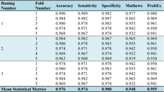
Xeon E5–1620 3.5 GHz processor, 64 GByte. The results of FF-ELM is given in Table 2.

Table 2 The performance of the FF-ELM Runing

Number Fold Number Accuracy Sensitivity Specificity Mathews ProbEx

1 1 0.990 0.989 0.992 0.977 0.980 2 0.984 0.982 0.987 0.965 0.969 3 0.980 0.978 0.983 0.955 0.961 4 0.974 0.971 0.978 0.942 0.950 5 0.969 0.967 0.974 0.932 0.941 2 1 0.984 0.982 0.987 0.965 0.969 2 0.980 0.978 0.983 0.955 0.961 3 0.974 0.971 0.978 0.942 0.950 4 0.969 0.967 0.974 0.932 0.941 5 0.963 0.960 0.969 0.919 0.930 3 1 0.974 0.971 0.978 0.942 0.950 2 0.980 0.978 0.983 0.955 0.961 3 0.974 0.971 0.978 0.942 0.950 4 0.984 0.982 0.987 0.965 0.969 5 0.969 0.967 0.974 0.932 0.941

Mean Statistical Metrics 0.976 0.974 0.980 0.948 0.955

In order to exactly evaluate the performances of the FF-ELM, standard ELM and BP-ANN, the training and test process were conducted with identical experiment design given in [21] and the mean values of the performance metrics that are accuracy, sensitivity and specificity were calculated for each experiment. The comparison of the mean performance metrics among to FF-ELM, ELM [21] and BP-ANN [21] is shown in Figure 3. According to mean results of accuracy, sensitivity and specificity metrics given in the Figure 3, FF-ELM shows the superior performance in comparison to the ELM and BP-ANN. However, the performance of standard ELM in terms of accuracy metric for experiment 4 is slightly better than other. The standard ELM has also comparatively good performance in for experiment 5 in the sensitivity and experiment 4 in the specificity, respectively. The comparison mean metric results of the FF-ELM with standard ELM and BP-ANN methods can be seen in Table 2 and to obtain obvious view in evaluating performance of the FF-ELM, standard ELM and BP-ANN methods, the performance metrics given in Table 2 are converted to the graphic charts. Fig. 3 displays the whole sensitivity, specificity, and accuracy average rates between BP ANN and ELM ANN. As examined the performance results given in Table 3 and Figure 3, FF-ELM ANN were generally better than standard ELM and BP-ANN.

(c)

Figure 3. The comparison of the mean performance metrics among to FF-ELM, ELM [21] and BP-ANN [21]: (a) Accuracy, (b)

Sensitivity and (c) Specificity

Table 3 The comparative performance of the FF-ELM, standard ELM and BP-ANN Methods _Accuracy Mean _Sensitivity Mean _Specificity Mean _Mathews Mean _ProbEx Mean

FF-ELM 0.976 0.974 0.980 0.948 0.955

ELM [21] 0.964 0.948 0.974 - -

ANN [21] 0.921 0.943 0.980 - -

Figure 4. Overall mean rates of the proposed the FF-ELM, standard ELM and BP-ANN

4. Conclusion

The performance of the FF-ELM was generally better than standard ELM and BP-ANN in diagnosis of the breast cancer disease. Though the overall mean specificity rate of the FF-ELM was slightly lower than BP ANN, it can be seen that the proposed FF-ELM was pretty the enhanced the sensitivity and accuracy rates. According to the achieved performance metric results, it can be concluded that the FF - ELM ANN has a better classification model than ELM and BP-ANN in diagnosing breast cancer disease based on Breast Cancer Wisconsin Dataset.

Kaynakça

[1] Subashini, T. S.; Ramalingam, V.; Palanivel, S., “Breast mass classification based on cytological patterns using RBFNN and SVM”, Expert Syst. Appl., 2009, 36 (3): 5284–5290.

[2] The American Cancer Society, What is Breast Cancer.

[3] Akay, M. F., “Support vector machines combined with feature selection for breast cancer diagnosis”, Expert Syst. Appl., 2009, 36(2), 3240–3247.

[4] West, D.; Mangiameli, P.; Rampal, R.; West, V., “Ensemble strategies for a medical diagnostic decision support system: A breast cancer diagnosis application”, Eur. J. Oper. Res., 2005, 162(2), 532–551.

[5] Brause, R. W., “Medical Analysis and Diagnosis by Neural Networks”, In Proceeding ISMDA’01 Proceedings of the Second International Symposium on Medical Data Analysis, Madrid, Spain, 1–13, 2001.

[6] P. Kshirsagar; N. Rathod, “Artificial neural network”, International Journal of Computer Applications, 2012, NCRTC(2), 12–16. [7] N. Gupta, “Artificial neural network”, Network and Complex Systems, 2013, 3(1), 24 – 28.

[8] Huang, G.-B.; Chen, L., “Convex incremental extreme learning machine.”, Neurocomputing, 2007,70(16), 3056-3062.

[9] Huang, G.-B.; Chen, L., “Enhanced random search based incremental extreme learning machine.”, Neurocomputing, 2008, 71(16), 3460-3468.

[10] Huang, G.-B.; Chen, L.; Siew, C. K., Universal approximation using incremental constructive feedforward networks with random hidden nodes., IEEE Trans. Neural Networks, 2006, 17(4), 879-892.

[11] Liu, X.; Lin, S.; Fang, J.; Xu, Z., “Is extreme learning machine feasible? A theoretical assessment (Part I). IEEE Transactions on Neural Networks and Learning Systems, 2015, 26(1), 7-20.

[12] Huang, G.-B.; Zhou, H.; Ding X., Zhang R., “Extreme learning machine for regression and multiclass classification”, IEEE Transactions on Systems, Man, and Cybernetics, Part B (Cybernetics), 2012, 42(2), 513-529.

[13] Suykens, J. A.; Vandewalle, J., “Least squares support vector machine classifiers. Neural processing letters”, 1999, 9(3), 293-300. [14] Cortes, C.; Vapnik, V., “Support vector machine”, Machine learning, 1995, 20(3), 273-297.

[15] Abdolmaleki, P.; Buadu, L.D.; Naderimanesh, H., “Feature extraction and classification of breast cancer on dynamic magnetic resonance imaging using artificial neural network”, Elsevier, Cancer Letters, 2001, 171 (2), 183-191.

[16] Fogel, D. B.; Wasson, E.C.; Boughton, E.M.; Porto, V.W., “A step toward computer assisted mammography using evolutionary programming and neural Networks”, Cancer Letters, 1997, 119(1), 93-97.

[17] Revett, K.; Gorunescu, F.; Gorunescu, M.; El-Darzı E.; Ene, M., “A breast cancer diagnosis system: a combined approach using rough sets and probabilistic neural Networks”, Computer as a tool Eurocon 2005, Belgrade, 2005, 1124- 1127.

[18] Gorunescu, M.; Gorunescu, F.; Revett, K., “Investigating a Breast Cancer Dataset Using a Combined Approach: Probabilistic Neural Networks and Rough Sets”, Proc. 3rd ACM International Conference on Intelligent Computing and Information Systems -ICICIS07, Cairo, Egypt, , 246-249, 2007.

[19] Hsiao, Y.H.; Huang, Y.L.; Liang, W.M.; Kuo S.J.; Chen D.R., “Characterization of benign and malignant solid breast masses: harmonic versus nonharmonic 3D power Doppler imaging”, Ultrasound Medicine & Biology, 2009, 35 (3), 353-359.

[20] Karapınar Şentürk, Z.; Şentürk, A., “Neural Networks with Breast Cancer Forecast”, El-Cezerî Journal of Science and Engineering, 2016, 3(2), 345-350.

[21] Prasetyo Utomo, C.; Kardiana, A.; Yuliwulandari, R., “Breast Cancer Diagnosis using Artificial Neural Networks with Extreme Learning Techniques”, International Journal of Advanced Research in Artificial Intelligence, 2014, 3(7), 10-14.

[22] Wolberg, W. H.; Mangasarian, O. L., “Multisurface method of pattern separation for medical diagnosis applied to breast cytology”, in Proceedings of the National Academy of Sciences, U.S.A., 87, 9193–9196, 1990.

[23] Yang, X.S., Nature-Inspired Metaheuristic Algorithms, Luniver Press, London, 2008.

[24] Yang, X. S., “Firefly algorithms for multimodal optimization”, Stochastic Algorithms: Foundations and Applications, SAGA, Lecture Notes in Computer Sciences 5792, 169–178, 2009.

[25] Łukasik, S.; Żak, S., “Firefly algorithm for continuous constrained optimization task”, Computational Collective Intelligence. Semantic Web, Social Networks and Multiagent Systems LNCS 5796, 97–106, 2009.

[26] Melamud, E.; Moult, J., “Evaluation of Disorder Predictions” in CASP5. Proteins 53:561–565, 2003.

[27] Yang, R. Z.; Thomso, R.; Mcneil, P.; Esnouf, R. M., “RONN: The bio-basis function neural network technique applied to the detection of natively disordered regions in proteins”, Bioinformatics, 2005, 21, 3369–3376.