Solutions Of Linear Fractional Differential Equations Of Order n-1<nq<n

(1)

RESEARCH ARTICLE

81

SOLUTIONS OF LINEAR FRACTIONAL DIFFERENTIAL EQUATIONS OF ORDER 𝒏 − 𝟏 < 𝒏𝒒 < 𝒏

Sertaç ERMAN1,* 1

Sakarya University of Applied Science, Faculty of Technology, Departement of Engineering Basic Science, Sakarya,

sertacerman@subu.edu.tr, ORCID: 0000-0002-3156-5173

Received Date:03.04.2020 Accepted Date:13.07.2020

ABSTRACT

In this study, the linear Caputo fractional differential equation of order 𝑛 − 1 < 𝑛𝑞 < 𝑛 is investigated. First, the solution of the equation of order 0 < 𝑞 < 1, with variable coefficients, is obtained by using the solution of differential equation of integer order which is the least integer greater than fractional order. Moreover, the solution of linear fractional differential equations of order 𝑛 − 1 < 𝑛𝑞 < 𝑛 is considered. The solutions of the equation are presented in terms of Mittag-Leffler function with three parameters. The main goal of this study is to present a closed-series form of the solutions. To demonstrate the accuracy and the effectiveness of the proposed approach, some numerical solutions are given.

Keywords: Fractional Differential Equation, Mittag-Leffler function, Three parameters 1. INTRODUCTION

The fractional derivative is very appropriate in modelling of physical pneumonias which involves past memory. Since fractional differential equations hold memory and are non-local in nature, it is known that mathematical models with fractional derivatives are more convenient and economical (See [1-8] and the references there in for more details). Due to this fact, they have been drawing increasing importance from scientist in past three decades (See [9-15] for some applications).

In this study, the Caputo fractional derivative is used. Since properties of Caputo fractional derivative are closed to properties of integer derivative, enormous studies on Caputo fractional differential equation and their applications can be found in the literature.

The linear Caputo fractional differential equation of order 0 < 𝑞 < 1, with variable coefficients, is considered and its solution is obtained as a series form. Next, the solution of linear sequential Caputo fractional differential equations of order 𝑛 − 1 < 𝑛𝑞 < 𝑛 is examined. The solutions of the equation are presented in terms of Mittag-Leffler function with three parameters.

2. PRELIMINARY DEFINITIONS

(2)

Erman. S., Journal of Scientific Reports-A, Number 45, 81-89, December 2020. 82 𝐷𝑞_{𝑢(𝑡) =} 1 Γ(𝑛 − 𝑞)∫ (𝑡 − 𝑠)𝑛−𝑞−1𝑢(𝑛)(𝑠)𝑑𝑠 𝑡 𝑡₀ 𝑓𝑜𝑟 𝑛 − 1 < 𝑞 < 𝑛, (1)

where 𝑛 is the smallest integer that exceeds 𝑞, 𝑡 ∈ [𝑡0, 𝑡0+ 𝑇] and 𝑢(𝑛)(𝑡) =𝑑

𝑛_𝑢(𝑡)

𝑑𝑡 .

The expression (1) is definition of Caputo (left-sided) fractional derivative of 𝑢(𝑡) for 𝑛 − 1 < 𝑞 < 𝑛 [7].

Moreover, it is clear that Caputo fractional derivative of order 0 < 𝑞 < 1 is defined as follows: 𝐷𝑞_{𝑢(𝑡) =} 1

Γ(1 − 𝑞)∫ (𝑡 − 𝑠)−𝑞𝑢′(𝑠)𝑑𝑠.

𝑡 𝑡0

(2)

Definition 2. The Mittag-Leffler function is defined by the series expansion as shown below

𝐸𝑞(𝑧) = ∑ 𝑧𝑘 Γ(𝑞𝑘 + 1) ∞ 𝑘=0 , (3) where 𝑞 > 0 [8].

In [7], some properties of Mittag-Leffler function and Caputo derivative are given as follows:

(i) 𝐷𝑛𝑞𝑢(𝑡) = 𝐷(𝑛−1)𝑞(𝐷𝑞)𝑢(𝑡) for 𝑛 − 1 < 𝑛𝑞 < 𝑛.

(ii) If 𝑞 = 1, 𝐸1,1(𝑡) = 𝑒𝑡, then it can be said that Mittag-Leffler function is generalization of usual

exponential function.

(iii) 𝐷𝑞(𝐸𝑞(𝑡𝑞)) = 𝐸𝑞(𝑡𝑞).

(iv) 𝐷𝑛𝑞(𝐸𝑞(𝑟𝑡𝑞)) = 𝑟𝑛𝐸𝑞(𝑟𝑡𝑞) where 0 < 𝑞 < 1, 𝑟 is a constant and 𝑛 ∈ ℕ.

Definition 3. The Mittag-Leffler function with two parameters is defined by the series expansion as shown below 𝐸𝛼,𝛽(𝑧) = ∑ 𝑧𝑘 Γ(𝛼𝑘 + 𝛽) , ∞ 𝑘=0 (4) where 𝛼, 𝛽 > 0 [8].

Definition 4. The Mittag-Leffler function with three parameters is defined by the series expansion as shown below 𝐸_𝛼,𝛽𝛾 (𝑧) = ∑ (𝛾)𝑘 𝑧𝑘 k! Γ(𝛼𝑘 + 𝛽) , ∞ 𝑘=0 (5) where 𝛼, 𝛽, 𝛾 > 0 and (𝛾)𝑘= 𝛾(𝛾 + 1) ⋯ (𝛾 + 𝑘 − 1) [8].

(3)

Erman. S., Journal of Scientific Reports-A, Number 45, 81-89, December 2020.

83 3. METHODOLOGY

In this study, fractional power series expansion method is used for linear Caputo fractional differential equation. The method is presented in [16] to obtain approximate solutions of fractional partial differential equations. The numerical results show that the method is significant method for fractional differential equation because of its simplicity and accuracy.

The main idea of the method is based on solving the differential equation of integer order which is the least integer greater than fractional order. Then, this solution is transformed the solution of fractional differential equation by using following series expansion:

𝑢(𝑡) ≅ 𝑇(𝑣(𝑡)) = ∑𝑣(𝑘)(0)𝑡 𝑘 𝑘! 𝑚−1 𝑘=0 + ∑ ∑𝑣(𝑚𝑘+𝑖)(0)𝑡 𝑘𝑞+𝑖 𝛤(𝑘𝑞 + 1 + 𝑖) 𝑚−1 𝑖=0 ∞ 𝑘=1 , (6) where 𝑢(𝑡) and 𝑣(𝑡) are solutions of fractional and ordinary differential equations respectively, 𝑚 is the least integer greater than fractional order 𝑞. For 0 < 𝑞 < 1, transformation (6) is expressed as follows: 𝑢(𝑡) ≅ 𝑇(𝑣(𝑡)) = ∑𝑣(𝑘)(0)𝑡 𝑘𝑞 𝛤(𝑘𝑞 + 1) ∞ 𝑘=0 . (7)

4. SOLUTION OF THE LINEAR FRACTIONAL DIFFERENTIAL EQUATION 4.1. Fractional Differential Equation of Order 𝟎 < 𝒒 < 𝟏

Let us consider the following linear differential equation with initial condition:

𝐷𝑞_{𝑢(𝑡) = 𝑝(𝑡, 𝑞)𝑢(𝑡) + 𝑓(𝑡, 𝑞), 𝑡𝜖[0, 𝑇], 𝑇 > 0}

𝑢(0) = 𝑢0,

(8) where 𝑝(𝑡, 𝑞) and 𝑓(𝑡, 𝑞) are continuous on 𝑡𝜖[0, 𝑇] for 0 < 𝑞 ≤ 1 and 𝑝(𝑡, 1), 𝑓(𝑡, 1) ∈ 𝐶∞_{([0, 𝑇], ℝ).}

In order to obtain the solution 𝑢(𝑡) of the problem (8) by using fractional power series expansion method, we need to have the solution of following ordinary differential equation

𝑣′_{(𝑡) = 𝑝̃(𝑡)𝑣(𝑡) + 𝑓̃(𝑡), 𝑡𝜖[0, 𝑇], 𝑇 > 0}

𝑣(0) = 𝑢0,

(9)

where 𝑝̃(𝑡) = 𝑝(𝑡, 1) and 𝑓̃(𝑡) = 𝑓(𝑡, 1).

The solution of problem (9) is well known and as follows:

𝑣(𝑡) = 𝑢0𝑒∫ 𝑝̃(𝑡)𝑑𝑡+ 𝑒∫ 𝑝̃(𝑡)𝑑𝑡∫ 𝑓̃(𝜏)𝑒∫ 𝑝̃(𝜏)𝑑𝜏𝑑𝜏 𝑡

0

(4)

84

By plugging the following derivatives of the solution 𝑣(𝑡) at 𝑡 = 0 𝑣(0) = 𝑢0 𝑣(𝑛)_{(0) = ∑ (}𝑛 − 1 𝑘 ) 𝑝̃(𝑘)(0)𝑣(𝑛−1−𝑘)(0) + 𝑓̃(𝑛−1)(0) 𝑛−1 𝑘=0 (11)

into transformation (7), the solution 𝑢(𝑡) of the problem (8) is obtained as follows: 𝑢(𝑡) ≅ 𝑢0+ ∑ ∑ (( 𝑛 − 1 𝑘 ) 𝑝̃(𝑘)(0)𝑣(𝑛−1−𝑘)(0) + 𝑓̃(𝑛−1)(0)) 𝑡𝑛𝑞 𝛤(𝑛𝑞 + 1) 𝑛−1 𝑘=0 . ∞ 𝑛=1 (12)

If 𝑝(𝑡, 𝑞) = 𝜆 is a constant in problem (8), the solution of problem (9) is obtained as follows: 𝑣(𝑡) = 𝑢0𝑒𝜆𝑡+ 𝑒𝜆𝑡∫ 𝑓̃(𝜏)𝑒𝜆𝜏𝑑𝜏

𝑡

0

. (13)

Moreover, derivatives of 𝑣(𝑡) are formed as follows: 𝑣(𝑛)_{(0) = 𝜆}𝑛_𝑢

0+ ∑ 𝜆𝑛−𝑘𝑓̃(𝑘−1)(0) 𝑛

𝑘=1

. (14)

Thus, by using transformation (7), the solution 𝑢(𝑡) of the problem (8) for 𝑝(𝑡, 𝑞) = 𝜆 (constant) is obtained in the following form:

𝑢(𝑡) ≅ 𝑢0𝐸𝑞(𝜆𝑡𝑞) + ∑ ∑ (𝜆𝑛−𝑘𝑓̃(𝑛−1)(0)) 𝑡𝑛𝑞 𝛤(𝑛𝑞 + 1) 𝑛 𝑘=1 ∞ 𝑛=1 . (15)

Additionally, for 𝑝(𝑡, 𝑞) = 𝜆, the problem (8) is investigated in [5,6] and its solution is presented in the following explicit form

𝑢(𝑡) = 𝑢0𝐸𝑞(𝜆𝑡𝑞) + ∫ (𝑡 − 𝑠)𝑞−1𝐸𝑞,𝑞(𝜆(𝑡 − 𝑠)𝑞)𝑓(𝑠, 𝑞)𝑑𝑠 𝑡

0 .

(16)

Hence, because of existence and uniqueness of the solution, the solution (15) equals to the solution (16) and this equality implies the following proposition.

Proposition 1. Let 𝑓(𝑡, 𝑞) be continuous on 𝑡𝜖[0, 𝑇] for 0 < 𝑞 ≤ 1 and 𝜆 ∈ ℝ. The following equality is satisfied ∫ (𝑡 − 𝑠)𝑞−1_𝐸 𝑞,𝑞(𝜆(𝑡 − 𝑠)𝑞)𝑓(𝑠, 𝑞)𝑑𝑠 ≅ ∑ ∑ (𝜆𝑛−𝑘_𝑓̃(𝑛−1)_(0))𝑡𝑛𝑞 𝛤(𝑛𝑞 + 1) 𝑛 𝑘=1 ∞ 𝑛=1 𝑡 0 , (17)

(5)

85 where 𝑓̃(𝑡) = 𝑓(𝑡, 1) ∈ 𝐶∞_{([0, 𝑇], ℝ) .}

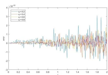
In order to show efficiency of the method, Proposition 1 is used. In Figure 1 and Figure 2, numerical simulations of the difference of both side of the equality (17) are given for some values of 𝑞 and functions 𝑓(𝑡, 𝑞) =_𝛤(𝑞+1)𝑡𝑞 and (𝑡, 𝑞) =_{𝛤(2𝑞+1)}𝑡2𝑞 .

Figure 1: When 𝑞 = 0.2, 0.4, 0.6, 08, the graph of difference of both side of the equality (17) for function 𝑓(𝑡, 𝑞) =_𝛤(𝑞+1)𝑡𝑞 and for 10 iteration

Figure 2: When 𝑞 = 0.2, 0.4, 0.6, 08, the graph of difference of both side of the equality (17) for function 𝑓(𝑡, 𝑞) =_{𝛤(2𝑞+1)}𝑡2𝑞 and for 10 iteration

(6)

86

4.2. Fractional Differential Equation of Order 𝒎 − 𝟏 < 𝒎𝒒 < 𝒎

The following linear sequential fractional differential equation with initial conditions is investigated in this section.

𝐷𝑚𝑞_{𝑢(𝑡) + 𝑏}

𝑚−1𝐷(𝑚−1)𝑞𝑢(𝑡) + ⋯ + 𝑏1𝐷𝑞𝑢(𝑡) + 𝑏0𝑢(𝑡) = 0, 𝑡𝜖[0, 𝑇], 𝑇 > 0

𝑢(0) = 𝑢0, 𝐷𝑖𝑞𝑢(0) = 𝑢𝑖,0, 𝑖 = 1,2, ⋯ , 𝑚 − 1 ,

(18)

where (𝑚 − 1) < 𝑚𝑞 < 𝑚 for 𝑚 ∈ ℕ and 𝑏𝑖∈ ℝ, 𝑖 = 1,2, ⋯ , 𝑚 − 1.

It is well known that the solutions of equation (18) are given in the form of 𝑢 = 𝐸𝑞(𝑟𝑡𝑞) where 𝑟 is

the solution of the corresponding characteristic equation of the following form:

𝑃(𝑟) = 𝑟𝑚_{+ 𝑏}

𝑚−1𝑟𝑚−1+ ⋯ + 𝑏1𝑟 + 𝑏0= 0 . (19)

If equation (19) has 𝑘 distinct roots 𝑟𝑖 for 𝑖 = 1,2, ⋯ , 𝑘 and 𝑘 ≤ 𝑚, a solution of the equation (18) is

obtained as follows:

𝑢(𝑡) = ∑ 𝑐𝑖𝐸𝑞(𝑟𝑖𝑡𝑞) 𝑘

𝑖=1

. (20)

Moreover, if equation (19) has 𝑘 coincident roots 𝑟0 for 𝑘 ≤ 𝑚, the solutions 𝑈𝑖(𝑡) of the equation

(18) can be constructed by the following recursive relation which is obtained from equation (16). 𝑈0(𝑡) = 𝐸𝑞,1(𝑟0𝑡𝑞)

𝑈𝑖(𝑡) = 𝑢0𝐸𝑞,1(𝑟0𝑡𝑞) + 𝑈𝑖−1(0) ∫ (𝑡 − 𝑠)𝑞−1𝐸𝑞,𝑞(𝜆(𝑡 − 𝑠)𝑞)𝑈𝑖−1(𝑠)𝑑𝑠 , 𝑡

0

(21) where 𝑖 = 1,2, ⋯ , 𝑘 − 1. Hence, the solution of the equation (18) is formed as follows:

𝑢(𝑡) = ∑ 𝑐𝑖𝑈𝑖(𝑡) 𝑘

𝑖=1

. (22)

In the following subsection, the closed forms of the solutions 𝑈𝑖(𝑡) related with the coincident roots of

characteristic equation are presented by using fractional power series method.

4.2.1. The closed forms of the solutions related with the m coincident roots

If the characteristic equation (19) has 𝑚 coincident roots 𝑟0, sequential differential equation (18)

reduced to

(𝐷𝑞_{− 𝑟}

0)(𝐷𝑞− 𝑟0)𝑚−1𝑢 = 0 . (23)

Letting (𝐷𝑞_{− 𝑟}

0)𝑚−1𝑢(𝑡) = 𝑈0(𝑡), the following fractional differential equation is obtained

(𝐷𝑞_{− 𝑟}

(7)

87

and by using the solution (15) with 𝑓(𝑡) = 0, the solution is obtained as follows:

𝑈0(𝑡) = 𝐸𝑞(𝑟0𝑡𝑞) . (24)

Moreover, letting (𝐷𝑞_{− 𝑟}

0)𝑚−2𝑢(𝑡) = 𝑈1(𝑡), the following fractional differential equation is

obtained

(𝐷𝑞_{− 𝑟}

0)𝑈1(𝑡) = 𝑈0(𝑡)

⇒ 𝐷𝑞_𝑈

1(𝑡) − 𝑟0𝑈1(𝑡) = 𝐸𝑞(𝑟0𝑡𝑞) (25)

Now, we solve the equation (25) by using fractional power series method. Let us consider the following ordinary differential equation which is obtained from equation (25) by equaling q to 1

𝑉′

1(𝑡) − 𝑟0𝑉1(𝑡) = 𝑒𝑟0𝑡. (26)

The solution of equation (26) is 𝑉1(𝑡) = 𝑡𝑒𝑟0𝑡. Then, applying transformation (7) to 𝑉1(𝑡) = 𝑡𝑒𝑟0𝑡, it

is obtained that

𝑈1(𝑡) =𝑡 𝑞

𝑞 𝐸𝑞,𝑞(𝑟0𝑡𝑞) , (27) which is exact solution of (25). Similarly, letting (𝐷𝑞_{− 𝑟}

0)𝑚−3𝑢(𝑡) = 𝑈2(𝑡), the following fractional

differential equation is obtained

(𝐷𝑞_{− 𝑟} 0)𝑈2(𝑡) = 𝑈1(𝑡) ⇒ 𝐷𝑞_𝑈 2(𝑡) − 𝑟0𝑈2(𝑡) = 𝑡𝑞 𝑞 𝐸𝑞,𝑞(𝑟0𝑡𝑞) . (28)

Also, the solution of the equation (28) is obtained in the form of Mittag-Leffler function with three parameters as follows:

𝑈2(𝑡) =𝑡 2𝑞

2𝑞𝐸𝑞,2𝑞2 (𝑟0𝑡𝑞) (29)

which is exact solution of (28). After applying m times these calculations recursively, the following solutions are obtained

𝑈1(𝑡) = 𝑡𝑞 𝑞 𝐸𝑞,𝑞1 (𝑟0𝑡𝑞) 𝑈2(𝑡) = 𝑡2𝑞 2𝑞𝐸𝑞,2𝑞2 (𝑟0𝑡𝑞) 𝑈3(𝑡) = 𝑡3𝑞 3𝑞𝐸𝑞,3𝑞3 (𝑟0𝑡𝑞) ⋮ . Moreover, these solutions can be written as follows:

(8)

88 𝑈𝑛(𝑡) =

𝑡𝑛𝑞

𝑛𝑞𝐸𝑞,𝑛𝑞𝑛 (𝑟0𝑡𝑞), 𝑛 = 1,2, ⋯ , 𝑚 − 1 . (30) Consequently, if characteristic equation (19) has 𝑚 coincident roots 𝑟0, there exists 𝑚 linearly

independent solutions as follows:

𝑈0(𝑡) = 𝐸𝑞(𝑟0𝑡𝑞), 𝑈𝑛(𝑡) = 𝑡𝑛𝑞 𝑛𝑞𝐸𝑞,𝑛𝑞𝑛 (𝑟0𝑡𝑞), 𝑛 = 1,2, ⋯ , 𝑚 − 1 . (31) 5. CONCLUSION

The approximate solution of linear Caputo fractional equation of order 0 < 𝑞 < 1 with variable coefficients is constructed as a series form. In this construction, the solution of differential equation of integer order which is the least integer greater than fractional order and its derivatives are used. Numerical results show that the approximation is significantly efficient when components of 𝑓(𝑡, 𝑞) are formed as 𝑡

𝑛𝑞

𝛤(𝑛𝑞+1) and 𝑝(𝑡, 𝑞) is constant in equation (8). Moreover, this result yields to obtain the

solution of linear sequential fractional differential equation of higher order with constant coefficient. Specifically, when characteristic equation has coincident root, the solutions are presented in terms of Mittag-Leffler function with three parameters.

REFERENCES

[1] Debnath, L., (2003), Recent applications of fractional calculus to science and engineering, International Journal of Mathematics and Mathematical Sciences, 54, 3413–3442.

[2] Ross, B., (1975), A Brief History and Exposition of the Fundamental Theory of Fractional Calculus. Fractional calculus and its Applications, Lecture notes in Mathematics, Springer: Berlin, Germany, 457, 1–36.

[3] Oldham, K.B., Spanier, J., (1974), The Fractional Calculus: Theory and Applications of Differentiation and Integration to Arbitrary Order, Academic Press: Newyork.

[4] Podlubny, I., (1998), Fractional Differential Equations, Volume 198: An Introduction to Fractional Derivatives, Fractional Differential Equations, to Methods of their solutions, Mathematics in Science and Engineering, Academic Press: San Diego.

[5] Podlubny, I., (2002), Geometric and physical interpretation of fractional integration and fractional differentiation, Fractional Calculus and Applied Analysis 5, 4, 367–386.

[6] Kilbas, A.A., Srivastava, H.M., Trujillo, J.J., (2006), Theory and Applications of Fractional Differential Equations, North-Holland Mathematics Studies, Elsevier: Amsterdam, The Netherlands.

(9)

89

[7] Deithelm, K., (2004), The Analysis of Fractional Differential Equations, Volume 2004 of Lecture Notes in Mathematics, Springer: Berlin, Germany.

[8] Gorenflo, R., Kilbas, A.A., Mainardi, F., Rogosin S.V., (2014), Mittag-Leffler Functions, Related Topics and Applications, Springer: Berlin, Germany.

[9] Pooseh, S., Rodrigues, H.S., Torres, D.F.M., (2011), Fractional Derivatives in Dengue Epidemics, AIP Conf. Proc., 1389, 739–742.

[10] Debnath, L., (2003), Recents Applications of Fractional Calculus to Science and Engineering, Int. J. Math. Appl. Sci, 54, 3413–3442.

[11] Singh, J., Kumar, D., Kılıçman, A., (2014), Numerical Solutions of Nonlinear Fractional Partial Differential Equations Arising in Spatial Diffusion of Biological Populations, Abstr. Appl. Anal., 2014, 535793.

[12] Koeller, R.C., (1984), Applications of Fractional Calculus to the Theory of Viscoelasticity, J. Appl. Mech., 51, 299–307.

[13] Saha, R.S., Bera, R.K., (2000), The random walk’s guide to anomalous diffusion: a fractional dynamics approach, Phys. Rep. 339, 2000, 1-77

[14] Waggas, G.A., (2010), Application of Fractional Calculus Operators for a New Class of Univalent Functions with Negative Coefficients Defined by Hohlov Operator, Math. Slovaca, 1, 75–82.

[15] Aliev, F.A., Aliev, N.A., Safarova, N.A., Gasimova K.G.,, Velieva N.I., (2018), Solution of Linear Fractional-Derivative Ordinary Differential Equations with Constant Matrix Coefficients, Applied and Computational Mathematics, 17, 3, 317-322

[16] Demir, A., Erman, S., Özgür, B., and Korkmaz, E., (2013), Analysis of fractional partial differential equations by Taylor series expansion, Boundary Value Problems, 68