IJISAE, 2015, 3(4), 136-139 | 136
Classification of Leaf Type Using Artificial Neural Networks
Ali Yasar
1, Ismail Saritas
2, M. Akif Sahman
3, A. Oktay Dundar
4Accepted 15
thAugust 2015
DOI: 10.18201/ijisae.49279
: 10.1039/b000000x
Abstract: A number of shape features for automatic plant recognition based on digital image processing have been proposed by Pauwels
et al. in 2009. Then Silva et al in 2014 have presented database comprises 40 different plant species. We performed in our study a classification process using dataset and artificial neural networks which have been prepared by Silva and et al. It has been determined that classification accuracy is over 92%.
Keywords: Artificial Neural Network, Leaf Dataset, ANN, Levenberg-Marquardt.
1. Introduction
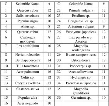
Data set which is prepared by Silva and et al consists of 40 different plants and a total of 340 data samples. Table 1 details each plant's scientific name and the number of leaf specimens available by species. Species numbered from 1 to 15 and from 22 to 36 exhibit simple leaves and species numbered from 16 to 21 and from 37 to 40 have complex leaves. That's why in our study 31 different classes (C), each plant's name and sample number have been shown in Table 1.
Table 1: Leaf database: plant species (C) and number of specimens available (#).
C Scientific Name # C Scientific Name #
1 Quercus suber 12 22 Primula vulgaris 12 2 Salix atrocinera 10 23 Erodium sp. 11 3 Populus nigra 10 24 Bougainvillea sp. 13
4 Alnus sp. 8 25 Arisarum vulgare 9
5 Quercus robur 12 26 Euonymus japonicas 12
6 Crataegus
monogyna
8 27 Ilex perado ssp. Azorica
11 7 Ilex aquifolium 10 28 Magnolia
soulangeana
12 8 Nerium oleander 11 29 Buxus sempervirens 12 9 Betulapubescens 14 30 Urtica dioica 12 10 Tilia tomentosa 13 31 Podocarpus sp. 11 11 Acer palmatum 16 32 Acca sellowiana 11
12 Celtis sp. 12 33 Hydrangea sp. 11
13 Corylus avellana 13 34 Pseudosasa japonica 11 14 Castanea sativa 12 35 Magnolia
grandiflora
11
15 Populus alba 10 36 Geranium sp. 10
16 Acer negundo 10
2. MATERIALS AND METHODS
2.1. Data Description
Each leaf specimen was photographed over a colored background using an Apple iPAD 2 device. The 24-bit RGB images recorded have a resolution of 720×920 pixels. Binary versions are provided for simple leaves. Fig. 1 provides an overview of the general aspect of the typical leaves of each plant.[1,2]
Figure 1. Leaf database overview
The provided data by Silva and et al comprises the following shape (attributes 3 to 9) and texture (attributes 10 to 16) features:
1.Class (Species) 2.Specimen Number 3.Eccentricity 4.Aspect Ratio 5.Elongation 6.Solidity 7.Stochastic Convexity 8.Isoperimetric Factor
9. Maximal Indentation Depth
10. Lobedness 11. Average Intensity 12. Average Contrast 13. Smoothness 14. Third moment 15. Uniformity 16. Entropy
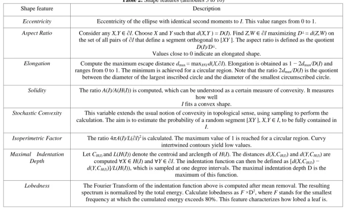
Let I denote an object of interest in a binary image, ∂I its border, D(I) its diameter, i.e., the maximum distance between any two points in ∂I and A(I) its area. Let A(H(I)) denote the area of the object’s convex hull (i.e. any ’optimal’ inscribing convex polygon) and L(∂I) the object’s contour length. Assume that the operator d(.) stands for the Euclidean distance. Table 2 details the definition of attributes 3 to 10.
_______________________________________________________________________________________________________________________________________________________________
1Guneysinir Vocational School, University of Selcuk, Konya, Turkey 2Faculty of Technology, University of Selcuk, Konya, Turkey 3Guneysinir Vocational School, University of Selcuk, Konya, Turkey 4Akoren Vocational School, University of Selcuk, Konya, Turkey *Corresponding Author: Email: [email protected]
Note: This paper has been presented at the International Conference on Advanced Technology&Sciences (ICAT'15) held in Antalya (Turkey), August 04-07, 2015
International Journal of
Intelligent Systems and Applications in Engineering
ISSN:2147-67992147-6799 www.ijisae.org Original Research Paper
IJISAE, 2015, 3(4), 136-139 | 137 Table 2: Shape features (attributes 3 to 10)
Shape feature Description
Eccentricity Eccentricity of the ellipse with identical second moments to I. This value ranges from 0 to 1. Aspect Ratio Consider any X,Y ∈ ∂I. Choose X and Y such that d(X,Y ) = D(I). Find Z,W ∈ ∂I maximizing D⊥ = d(Z,W) on
the set of all pairs of ∂I that define a segment orthogonal to [XY ]. The aspect ratio is defined as the quotient D(I)/D⊥.
Values close to 0 indicate an elongated shape.
Elongation Compute the maximum escape distance dmax = maxX∈I d(X,∂I). Elongation is obtained as 1 − 2dmax/D(I) and
ranges from 0 to 1. The minimum is achieved for a circular region. Note that the ratio 2dmax/D(I) is the quotient
between the diameter of the largest inscribed circle and the diameter of the smallest circumscribed circle. Solidity The ratio A(I)/A(H(I)) is computed, which can be understood as a certain measure of convexity. It measures
how well I fits a convex shape.
Stochastic Convexity This variable extends the usual notion of convexity in topological sense, using sampling to perform the calculation. The aim is to estimate the probability of a random segment [XY ], X,Y ∈ I, to be fully contained in
I.
Isoperimetric Factor The ratio 4πA(I)/L(∂I)2 is calculated. The maximum value of 1 is reached for a circular region. Curvy
intertwined contours yield low values. Maximal Indentation
Depth
Let CH(I) and L(H(I)) denote the centroid and arclength of H(I). The distances d(X,CH(I)) and d(Y,CH(I)) are computed ∀X ∈ H(I) and ∀Y ∈ ∂I. The indentation function can then be defined as [d(X,CH(I)) − d(Y,CH(I))]/L(H(I)), which is sampled at one degree intervals. The maximal indentation depth D is the
maximum of this function.
Lobedness The Fourier Transform of the indentation function above is computed after mean removal. The resulting spectrum is normalized by the total energy. Calculate lobedness as F ×D2, where F stands for the smallest
frequency at which the cumulated energy exceeds 80%. This feature characterizes how lobed a leaf is.
Attributes 11 to 16 are based on statistical properties of the intensity histograms of grayscale transformations of the original RGB images. The definition of each attribute is given in Table3.[1,2]
If Z is a random variable indicating image intensity, its nth moment around the mean is
), where m is the mean of Z, p(.) its histogram and L is the number of intensity levels.
Table 3: Texture features (attributes 11 to 16)
Texture feature Description
Average Intensity Average intensity is defined as the mean of the intensity image, m. Average Contrast Average contrast is the the standard deviation of the intensity im-
age, σ = pµ 2(z).
Smoothness Smoothness is defined as R = 1 − 1/(1 + σ2) and measures the relative smoothness of the intensities in a given
region. For a region of constant intensity, R takes the value 0 and R approaches 1 as regions exhibit larger disparities in intensity values. σ2 is generally normalized by (L − 1)2 to ensure that R ∈ [0,1].
Third moment µ3 is a measure of the intensity histogram’s skewness. This measure is generally normalized by (L − 1)2 like
smoothness. Uniformity
Defined as ), uniformity’s maximum value is reached when all intensity levels are equal.
Entropy A measure of intensity randomness.
2.2. Artificial Neural Network
Artificial Neural Networks have emerged as the simulation of the biological nervous system. A mode of operation of a computer by assimilating to the mode of operation of a brain, neural network model was developed. Learning in artificial neural network algorithms depend on previously acquired experiences. After removing the properties of a system even if an algorithm based on solution of system or it has a complex solution analysis, artificial neural networks can be applied to this system. Artificial neural networks are composed of neurons. These neurons can be connected into each other, even in a very complex way as in real nervous system. Each neuron has entries in the different weight and one output. For this purpose, total of inputs in the different weights is defined as follows [3].
Here; P is the number of inputs, w is the input weight, x is input, b is the value of the bias and neural network. The weighted inputs and sum of each neuron together with the bias are passed through the activation function and consequently output depend on that neuron is obtained. If we indicate activation function with "f", it is expressed as follows.
The activation function (activity function, φ) may be sigmoid function, threshold function or a hyperbolic tangent function according to the structure of the system. After the output has
IJISAE, 2015, 3(4), 136-139
obtained if the system is multilayer, the output of a neuron (y) may be an input (x) of a neuron. In this way, a multilayer neural network model is generated [4].
Figure 2. General Structure of Artificial Neural Network [5]
Artificial neural network model usually consists of three parts: the input layer, hidden layer and output layer. Each layer may consist of a lot of neurons. After information transmits from the input layer, it transmits activation function. Outputs of the input layer continues as the entry of the hidden layer. After this process, in result function once again evaluating the hidden output layer of activation functions, final output is obtained. The first step of learning in neural networks can be characterized as activation. Signals which enter nerve cell may activate cell signal. If total signal is as high as to fire the cell and get over threshold then the cell is active, but it is passive if not so. According to being active or passive of nerve cell, can be extrapolated if it can make classification or not. An artificial neural network cell which is capable of making classification for input patterns as 1 or 0, it is deemed to have decided setting value to pattern 1 or 0. ''Making decision'' "and" classifying ", are the cornerstones of the learning process [6].
2.3. Experimental Studies
Pauwels et al. in 2009 and Silva et al. in 2014 Leaf data sets have
been used downloading from
http://archive.ics.uci.edu/ml/datasets/Leaf. There are a total of 340 data. In the training phase, 289 randomly selected neural network, in the data testing phase 34 data, in the validation phase 17 data have been used. Our system is designed with Matlab R2014b ANN Toolbox and it consists 15 neuron, 1 input layer, a hidden layer consists of 23 neuron and 1 output layer. Levenberg-Marquardt algorithm is used during the training of the Neural Network. 2.3.1. Levenberg-Marquardt Algorithm
Basically, the Levenberg-Marquardt (LM) algorithm, based on the idea of Neighbourhood is a least squares maximum calculation method. This algorithm consists of the best features of Gauss-Newton and Steepest-Descent (Back Propagation) algorithms and eliminates the limitations of these two methods.
One of the problems encountered in the Gauss-Newton method is unable to calculate the inverse of Hessian matrix approximately. For solving this problem, in Levenberg-Marquardt algorithm a small μ constant is added to H Hessian matrix.
In the equation I is the unit matrix, μ is a small fixed number. W is the line vector which is created from all of the weight and can be expressed as follows:
J (W) is Jacobian matrix, and contains the first order derivatives based on values of weight and bias of errors and it is calculated as follows: Current error, the column vector and instant performance function E (W, n), including the sum of the squares of the error,
obtained by the above equation. Total performance J (W), ie, the mean square error is:
Updating of the weights is calculated as follows different from the Gauss-Newton.
ΔW is the amount of weight change. This work of algorithm can be summarized generally as follows:
1. Performance function E (W, n) is calculated,
2. It is started with a small μ value (μ = 0.01)
3. Being calculated ΔW, the next value of the performance
function is calculated.
4. If the next value of the performance function is greater than
current values, μ is increased 10-times.
5. The next value of the performance function is less than the
current value, μ is reduced 10-times ,
6. Weights are updated and gone to step 3.
In summary, the weights are set initial values and by calculating the total of squares of the errors, the process is continued. Each error term refers to the square of the difference between actual output and the target output. Having been obtained error terms for all data sets learning is provided LevenbergMarquardt method by implementing of step 1 to step 5 [7,8,9].
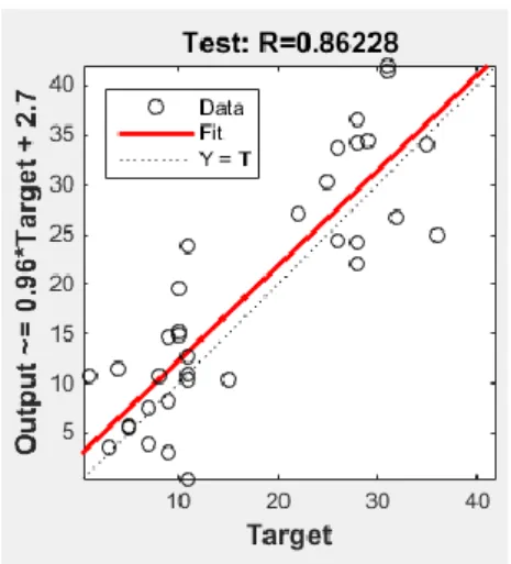
Our values which we have obtained as a result of our study can be seen more clearly from the following Fig.s.
In Fig. 3, Regression Graphic of Training Dataset
Figure 3. Training Regression
In Fig. 4, Regression Graphic of Test Dataset
IJISAE, 2015, 3(4), 136-139 Figure 4. Regression of Test Set
and in Fig. 5, Regression of Validation Dataset can be seen
Figure 5. Regression of Validation
Regression of Output can be seen in Fig. 6
Figure 6. Regression of Output
3.
Result and Discussion
MATLAB program is used for executing the process. The model uses the trainlm - Levenberg–Marquardt function for training. The MATLAB program randomly divides input variables and target
variables into three sets. 85 % of the samples are assigned to the training set, 5% to the validation set, and 10% to the test set. Many different functions such as ‘‘logsig”, “tansig”, and “purelin” were tested as transfer function for hidden layer and “purelin” function was used as the output layer transfer function. Learngdm (gradient descent with momentum weight and bias learning function) function was used as the adaption learning function and MSE and R was determined as the performance function.
4. Conclusions
In this study, it has been seen that artificial neural networks can be used in the classification process and good results can be obtained. When obtained results were considered, we obtained better results than study of "Pedro F.B. Silva, Andr´e R. S. Marca, and Rubim M. Almeida da Silva, called "Evaluation of Features for Leaf Discrimination" [1]. While Silva and et al have 87% classification success, in our study it can be seen that we have a classification success around 92%.
References
[1] “Evaluation of Features for Leaf Discrimination”, Pedro F. B. Silva, Andre R.S. Marcal, Rubim M. Almeida da Silva (2013), Springer Lecture Notes in Computer Science, Vol. 7950, 197-204.
[2] “Development of a System for Automatic Plant Species Recognition”, Pedro Filipe Silva,Disserta¸ca˜o de Mestrado (Master’s Thesis), Faculdade de Ciˆencias da Universidade do Porto. Available for download or online reading at http://hdl.handle.net/10216/67734
[3] Haykin, S., Neural networks a comprehensive foundation, 1994.
[4] Ertunç, H.M., Ocak, H., Aliustaoğlu, C., "ANN and ANFIS based multi-staged decision algorithm for the detection and diagnosis of bearing faults", Neural Comput and Application, 2012.
[5] Uğur A., KINACI A.C., “Yapay Zeka Teknikleri ve Yapay
Sinir Ağları Kullanılarak Web Sayfalarının
Sınıflandırılması”, 11.İnternet Konferansları, 2006. (in Turkish)
[6] Çelik E., Atalay M., Bayer H., “Yapay Sinir Ağlari Ve Destek Vektör Makineleri İle Deprem Tahmininde Sismik Darbelerin Kullanilmasi Earthquake Prediction Using Seismic Bumps With Artificial Neural Networks And Support Vector Machines”,2014.
[7] Özkan Ö., Yildiz M., Köklükaya E., “Fibromiyalji Sendromunun Teşhisinde Kullanilan Laboratuar Testlerinin Sempatik Deri Cevabi Parametreleriyle Desteklenerek Teşhis Doğruluğunun Arttirilmasi”2011. (in Turkish)
[8] Sağıroğlu, Ş., Beşdok, E., Erler, M., Mühendislikte yapay zeka uygulamaları-I, Ufuk Kitap Kırtasiye-Yayıncılık Tic. Ltd., 2003. (in Turkish)
[9] The MathWorks, Inc., MATLAB® Documentation Neural Network Toolbox Help, “Levenberg-Marquardt Algorithm”, Release 2009a, 2009.
![Figure 2. General Structure of Artificial Neural Network [5]](https://thumb-eu.123doks.com/thumbv2/9libnet/4967207.100458/3.892.86.407.143.358/figure-general-structure-artificial-neural-network.webp)