Computation of holographic patterns between tilted planes

(1)

Computation of Holographic Patterns Between Tilted Planes

Gökhan Bora Esmer and Levent Onural

Department of Electrical and Electronics Engineering Bilkent University, TR-06800, Ankara,

TURKEY

ABSTRACT

Computation of the diffraction pattern that gives the desired reconstruction of an object upon proper illumination is an important process in computer generated holography. A fast computational method, based on the plane wave decomposition of 3D field in free-space, is presented to find the desired diffraction pattern. The computational

burden includes two FFT algorithms in addition to a shuffling of the frequency components that needs an interpolation in the frequency domain. The algorithm is based on the exact diffraction formulation; there is no need for Fresnel or Fraunhofer approximations. The developed model is utilized to calculate the scalar optical diffraction between tilted planes for monochromatic light. The performance of the presented algorithm

is satisfactory for tilt angles up to 600.

Keywords: Digital Holography, Diffraction, Plane Wave Decomposition

1. INTRODUCTION

The holography is based on duplication of information-carrying optical waves which come from a 3D scene in the absence of the original source. Holography can be easily understood by the diffraction principles of optical waves and mathematics of the interference.

One of the important problems in digital holography is the computation of diffraction pattern due to an

object. Calculation of the diffraction pattern between tilted planes is a challenging problem. Several researchers proposed methods to solve the tilted plane problem. The method proposed by Ganci is based on the Fiaunhofer approximation and deals with a simplified representation of diffraction of a plane wave passing through a tilted

slit.1 Rabal et al. offered a generalization of the method proposed by Ganci.2 Rabal et al. examine the ampli-tude of diffraction pattern due to a tilted aperture by using Fraunhofer approximation. They take the Fourier transform of the tilted plane transmission function in its own coordinate system. The relation of Fourier

trans-form coordinates to spatial coordinates of the final output plane is obtained by using coordinate transtrans-formation.2

Leseberg and Frére use Fresnel approximation to find the diffraction pattern of a tilted plane.3 Later Frére and Leseberg suggested another method to approximate diffraction patterns of off-axis tilted objects.4 Then

Tommasi and Bianco offered a method which is based on the relation between the plane wave spectrum of rotated planes.5 They also used the proposed technique to calculate computer generated holograms of off-axis objects.6

Then, a method which is based on Rayleigh-Sommerfeld scalar diffraction integral is presented by Delen and Hooker.7 Matsushima et al. use the same scalar diffraction method as Delen and Hooker but Matsiishima et

al. use several interpolation algorithms in their method.8

The method used in this paper is based on the algorithm proposed by Delen and Hooker.7 Another property

of the method we use in this paper is the incoming angle of light that illuminates the input plane is taken as

constant. Moreover, discrete implementation of the method is obtained by sampling both spatial and frequency

domains and it causes to deal with periodic input and diffraction patterns. As a result of this, we have two limitations in calculation of the diffraction pattern. These limitations are on the distance between input and

observation plane, and tilt angle of the planes.

Further author information: Send correspondence to Gökhan Bora Esmer: borahan©ee.bilkent.edu.tr. Levent Onural: onural@ee.bilkent.edu.tr

www.3dtv-reseach.org

Computation of Holographic Patterns Between Tilted Planes

Gökhan Bora Esmer and Levent Onural

Department of Electrical and Electronics Engineering Bilkent University, TR-06800, Ankara,

TURKEY

ABSTRACT

Computation of the diffraction pattern that gives the desired reconstruction of an object upon proper illumination is an important process in computer generated holography. A fast computational method, based on the plane wave decomposition of 3D field in free-space, is presented to find the desired diffraction pattern. The computational

burden includes two FFT algorithms in addition to a shuffling of the frequency components that needs an interpolation in the frequency domain. The algorithm is based on the exact diffraction formulation; there is no need for Fresnel or Fraunhofer approximations. The developed model is utilized to calculate the scalar optical diffraction between tilted planes for monochromatic light. The performance of the presented algorithm

is satisfactory for tilt angles up to 600.

Keywords: Digital Holography, Diffraction, Plane Wave Decomposition

1. INTRODUCTION

The holography is based on duplication of information-carrying optical waves which come from a 3D scene in

the absence of the original source. Holography can be easily understood by the diffraction principles of optical

waves and mathematics of the interference.

One of the important problems in digital holography is the computation of diffraction pattern due to an

object. Calculation of the diffraction pattern between tilted planes is a challenging problem. Several researchers proposed methods to solve the tilted plane problem. The method proposed by Ganci is based on the Fiaunhofer approximation and deals with a simplified representation of diffraction of a plane wave passing through a tilted

slit.1 Rabal et al. offered a generalization of the method proposed by Ganci.2 Rabal et al. examine the ampli-tude of diffraction pattern due to a tilted aperture by using Fraunhofer approximation. They take the Fourier transform of the tilted plane transmission function in its own coordinate system. The relation of Fourier

trans-form coordinates to spatial coordinates of the final output plane is obtained by using coordinate transtrans-formation.2

Leseberg and Frére use Fresnel approximation to find the diffraction pattern of a tilted plane.3 Later Frére and Leseberg suggested another method to approximate diffraction patterns of off-axis tilted objects.4 Then

Tommasi and Bianco offered a method which is based on the relation between the plane wave spectrum of rotated planes.5 They also used the proposed technique to calculate computer generated holograms of off-axis objects.6

Then, a method which is based on Rayleigh-Sommerfeld scalar diffraction integral is presented by Delen and Hooker.7 Matsushima et al. use the same scalar diffraction method as Delen and Hooker but Matsiishima et

al. use several interpolation algorithms in their method.8

The method used in this paper is based on the algorithm proposed by Delen and Hooker.7 Another property

of the method we use in this paper is the incoming angle of light that illuminates the input plane is taken as

constant. Moreover, discrete implementation of the method is obtained by sampling both spatial and frequency

domains and it causes to deal with periodic input and diffraction patterns. As a result of this, we have two limitations in calculation of the diffraction pattern. These limitations are on the distance between input and

observation plane, and tilt angle of the planes.

Further author information: Send correspondence to Gökhan Bora Esmer: borahan©ee.bilkent.edu.tr. Levent Onural: onural@ee.bilkent.edu.tr

(2)

2. MATHEMATICAL MODEL IN THE CONTINUOUS DOMAIN

Off-axis holography uses the physical phenomena of interference and diffraction. The diffraction pattern due to

an object is represented by /'(x), and R(x, y) is the reference beam we use to modulate the diffraction pattern

'(x)

. Thereference beam is taken as a plane wave whose amplitude is Ro and it is incident upon the recording

medium with its direction of propagation in the x-z plane. The mathematical expression of R(x, y) is

R(x,y) =Roexp(jkxsin9) (1)

where k is the wave number, 0 is the angle between propagation direction of reference beam and z axis.

The scalar diffraction theory for monochromatic coherent light is formulated not only in the spatial domain but also in frequency domain.9 Fourier analysis of the input field provides the complex amplitude of the plane

waves which propagate in different directions. The relation between 3D field in space, /'(x), and the complex amplitudes of the plane waves obtained by Fourier transform of the 2D input field which is given as A(k, k) is

(x)

= J

A(k, k) exp (jkTx)dkdk

(2)

where x is the position vector given as [

x

y z jT The parameter k is the 3D wave vector whose components

k, k and k represent the spatial frequencies of the propagating wave along the x, y and zaxis. _Replacing

z= 0into Eq 2 gives the field on the input plane z =0as

f(x,y)

(x,y,O)

=

_{fA(kxky)exP{(kxx+}

ky)}dkdk . (3)

Weobserve from Eq 3 that A(k, k)(2ir)2 equals to the 2D Fourier transform (FT) of the field on z =_{Q plane.1°}

We define z =0plane as the input plane which is shown in figure 1(a). The input plane is spanned by =(1,0,0)

and =

_(0,1, 0) unit vectors. The observation plane is spanned by

x'=Rx+b

(4)

asx takes values over the input plane. The parameter R is a rotation matrix and b is the translation vector in

space. Eq 4 provides to have tilted input or observation planes The rotation matrix R is defined as

Ti1 T12 Ti3

R

=

_'21 T22 T23 . (5)

T31 T32 7'33

Theobservation plane is spanned by x' =Ráand y' =

R

unit vectors originating from point b.

To obtain the diffraction pattern on the observation plane, x' =

Rx

+ b is substituted into Eq 2. Then we

get the mathematical expression of the diffraction pattern on observation plane as

g(x',y')

(R

[

] +b)

=

fA(RkF)exp{j(kFTx))}exp{j(RkF)Tb}J(kz,k)dkdk (6)

where k' represents the propagation direction of plane waves with respect to the observation plane. The relation

between k and k' represents a frequency mapping operation and it is given as k =Rk'. Therefore, each plane wave component of the 3D field generates a different 2D Fourier component over the input and output planes: the amplitude and the frequency of a component over the input plane correspond to another 2D frequency (due

to the tilt), and the amplitude at this new frequency is modified both by the Jacobian correction factor, and the propagation distance. As an example, let us consider a plane wave propagating from the input plane to the observation plane along the z-axis and it is parallel to the input plane. The DC term (k =0,

k =

0) at the

object plane is mapped to k = sin_{45°, k =}0at the observation plane when tilt angle around the y-axis is

2. MATHEMATICAL MODEL IN THE CONTINUOUS DOMAIN

Off-axis holography uses the physical phenomena of interference and diffraction. The diffraction pattern due to

an object is represented by i/'(x), and R(x, y) is the reference beam we use to modulate the diffraction pattern

b(x). The reference beam is taken as a plane wave whose amplitude is Ro and it is incident upon the recording medium with its direction of propagation in the x-z plane. The mathematical expression of R(x, y) is

R(x, y) =R0exp (jkx sin 9) (1)

where k is the wave number, 0 is the angle between propagation direction of reference beam and z axis.

The scalar diffraction theory for monochromatic coherent light is formulated not only in the spatial domain but also in frequency domain.9 Fourier analysis of the input field provides the complex amplitude of the plane

waves which propagate in different directions. The relation between 3D field in space, '(x), and the complex amplitudes of the plane waves obtained by Fourier transform of the 2D input field which is given as A(k, k) is

(x) =

_J

A(k, k) exp (jkTx)dkdk

(2)

where x is the position vector given as [

x

y z JT• The parameter k is the 3D wave vector whose components k, k and k represent the spatial frequencies of the propagating wave along the x, y and z axis. Replacing

z =

0into Eq 2 gives the field on the input plane z =0as

f(x,y)

(x,y,O)

=

fA(kxky)exP{(kxx

+ ky)}dkdk . (3) Weobserve from Eq 3 that A(k, k)(2rr)2 equals to the 2D Fourier transform (FT) of the field on z =_{Q plane.'°}

We define z =0plane as the input plane which is shown in figure 1(a). The input plane is spanned by =(1,0,0)

and =

_(0,1, 0) unit vectors. The observation plane is spanned by

x'=Rx+b

(4)

as x takes values over the input plane. The parameter R is a rotation matrix and b is the translation vector in space. Eq 4 provides to have tilted input or observation planes The rotation matrix R is defined as

Ti1 T12 Ti3

R = _r2i r22 r23 . (5)

r31 T32 T33

Theobservation plane is spanned by x' =Ráand y' =

R

unit vectors originating from point b.

To obtain the diffraction pattern on the observation plane, x' =

Rx

+ b is substituted into Eq 2. Then we

get the mathematical expression of the diffraction pattern on observation plane as

g(x', y')

(R

[

] +

b) =

JA(Rk')

exp {j(k/Tx))} exp {j(RkF)Tb}J(k, k)dkdk (6)

where k' represents the propagation direction of plane waves with respect to the observation plane. The relation

between k and k' represents a frequency mapping operation and it is given as k =Rk'. Therefore, each plane wave component of the 3D field generates a different 2D Fourier component over the input and output planes: the amplitude and the frequency of a component over the input plane correspond to another 2D frequency (due

to the tilt), and the amplitude at this new frequency is modified both by the Jacobian correction factor, and the propagation distance. As an example, let us consider a plane wave propagating from the input plane to the observation plane along the z-axis and it is parallel to the input plane. The DC term (k =0,

k =

0) at the

(3)

taken as 45°. The function J(k, k) is the Jacobian and equals to . Please

note that k is a function of k

and k,; and the relation is given as

k =

_{()2 _ (k)2}

-

(k)2 (7)

Furthermore, k is also a function of k and k. By using the frequency mapping relation k =Rk', we can

obtain k from k and k,.

The frequency mapping operation is performed on a surface of a sphere (the so called Ewald sphere) defined

by the term k2

k2

—

_k2.

_{The radius of the sphere is determined by the parameter k which equals to}

The term exp {jkTb} which is given in Eq 6 provides the phase delay for each plane wave and we represent

it by the function H(k', R, b). H(k', R, b) is found as

H(k', R, b) =exp

{j(RkF)Tb} .

(8)

Combining Eq 3 and 6, we get the relation between f(x,_y) and g(x',y') as

g(x',y') =

_{1(k,k)(x',y')}

_{{42(Xy)(kk){f(x,}

_{y)}k.,H(k', R,}

_{b) %}

_}

(9) whereoperator F is the 2D Fourier transformation. The frequency mapping operation is represented by k —iRk'.

The operation (k,, k,) —+ (x', y') isthe inverse Fourier transform between the frequency domain given by (k,, k,)

and the spatial domain represented by (x', y'), and similarly, the operation (x, y) —i(ks,k) provides the forward

Fourier transform between the spatial domain (x, y) and the frequency domain (ks, ku).

3. CORRESPONDING DISCRETE MODEL

Formulation of scalar optical diffraction between tilted planes in continuous domain is given by Eq 6. However,

we have to discretize the model to generate the digital simulator. Therefore, we have to sample equations 3

and 6. Sampling in both spatial and frequency domains results in implicit periodic input and output. Therefore,

the discrete domain model can handle only periodic patterns. The implemented simulator displays only one period of the input and output patterns. Sampling points in spatial and frequency domain are set as

x=Xn8, y=Xm3

2ir 2ir

(10)

where X is the sampling period, N is an integer which gives the period of the discrete input and output patterns.

The variables n3, m3, n1 and mf are integers in the range [—N/2, N/2). The variables X and N determines the distance between the input and the observation planes implicitly. When the distance between the input and

the observation planes is assigned not larger than

,

thecalculated diffraction pattern is similar non-periodic case. The deviation is caused by the higher frequencies. Moreover, deviation will increase when the tilt angle is increased. Again, the high frequency components are the cause of the deviation.

The variable k is a function of k and k, as mentioned in the continuous model and the discrete version of

k is

_{_____________}

k =

_{2_nf2mf2}

(11)

where 3 is equal to

Uniform sampling of k and k causes to have larger angles between consecutive plane wave components as

the wave vector of the plane wave moves away from the z-axis. This in turn compensates for the Jacobian term that appears in the continuous formulation, and thus, the Jacobian term does not appear in the discrete versions.

The mathematical expression of the sampled reference beam is obtained as

R(n,m) =

RoexpjFn (12)

taken as 45°. The function J(k, k) is the Jacobian and equals to . Please

note that k is a function of k

and k ; and the relation is given as

k

=

()2

_{_ (k)2- (k)2} ₍₇₎

Furthermore, k is also a function of k and k. By using the frequency mapping relation k =Rk', we can

obtain k from k and k,.

The frequency mapping operation is performed on a surface of a sphere (the so called Ewald sphere) defined

by the term k2

k2

—

1c2 . Theradius of the sphere is determined by the parameter k which equals to .

Theterm exp {jkTb} which is given in Eq 6 provides the phase delay for each plane wave and we represent

it by the function H(k', R, b). H(k', R, b) is found as

H(k', R, b) =exp

{j(RkF)Tb} .

(8)

Combining Eq 3 and 6, we get the relation between f(x,_y) _{and g(x',y') as}

g(x',

y') = :F-'

_{(k,k)—(x',y') {42(Xy)(k ,k) {f(x,}y)}

_k—Rk1'

R,

_{b) }}

(9) where operator F is the 2D Fourier transformation. The frequency mapping operation is represented by k —iRk'.

The operation (k, k,) —+(x', y') isthe inverse Fourier transform between the frequency domain given by (k, k,)

and the spatial domain represented by (x', y'), and similarly, the operation (x, y) —i(kr,k) provides the forward

Fourier transform between the spatial domain (x, y) and the frequency domain (kr, ku).

3. CORRESPONDING DISCRETE MODEL

Formulation of scalar optical diffraction between tilted planes in continuous domain is given by Eq 6. However,

we have to discretize the model to generate the digital simulator. Therefore, we have to sample equations 3

and 6. Sampling in both spatial and frequency domains results in implicit periodic input and output. Therefore,

the discrete domain model can handle only periodic patterns. The implemented simulator displays only one period of the input and output patterns. Sampling points in spatial and frequency domain are set as

x=Xn8, y=Xm8

2rr 2rr

(10)

where X is the sampling period, N is an integer which gives the period of the discrete input and output patterns.

The variables n ,m3, Thfand mf are integers in the range [—N/2, N/2) . Thevariables X and N determines the distance between the input and the observation planes implicitly. When the distance between the input and

the observation planes is assigned not larger than

,

thecalculated diffraction pattern is similar non-periodic case. The deviation is caused by the higher frequencies. Moreover, deviation will increase when the tilt angle is increased. Again, the high frequency components are the cause of the deviation.

The variable k is a function of k and k ,asmentioned in the continuous model and the discrete version of

k is

_{_____________}

kZ=2_nf2_mf2

(11)

where 3 is equal to

Uniform sampling of k and k causes to have larger angles between consecutive plane wave components as

the wave vector of the plane wave moves away from the z-axis. This in turn compensates for the Jacobian term that appears in the continuous formulation, and thus, the Jacobian term does not appear in the discrete versions.

The mathematical expression of the sampled reference beam is obtained as

(4)

where F is defined as X sinG.

Input pattern f(x, y) is sampled by using Eq 10 and an NxN input array is obtained. A sampled input

pattern is shown in Figure 1(a). The variables n8 and m8 are in the range [—N/2, N/2), hence f(x, y) is in the

range [=- ,

). Then

a new array fD(fls, m8) is defined and it is obtained from the samples of f(x, y) in the

range [0, NX). Plane wave coefficients which suppose in 3D space to give the 2D pattern over the input plane AD(nf, m1) is computed as

1

I

\ ir2 r rrr I.e I

11Dflf,mf) = 1v L/U NxN'JDfls,m8

These coefficients give the amplitudes of the frequency components of the signal on the input plane. The frequency mapping operation is used to find the frequency components of the signal on the observation plane.

The frequency coefficients of the signal on the observation plane are defined as

—

I, F' ill F\ IF

F \

A1,Dnf,mf) = ADunf, mf), Vflf, mf)) (14)

where (n, m'j) is in the range [, ) and u(n, m's) and v(n,,, m'j) are computed as

u(n, m) = (n + s)rii + (m'f + t)r12 +

(n'1 + s)2 —(m'f+ t)2r13

v(n, m) = (n + S)T21 + (m'f + t)r22 + 2 (n'1 + s)2 —

(rn'1+ t)2r23 (15)

where s and t are chosen to be equal to r31 and r32, respectively.

Generally, f(x, y) is a base-band signal so its frequency components A(k, k) are concentrated around the origin, (kr, k) = (0, 0). As a result of the frequency mapping operation, k' = R1k, the frequency concentration moves to around (k, k) = (r3l, r32j3). Therefore, the signal in Eq 6 becomes a band-pass signal. To avoid

dealing with unnecessarily large discrete FT (DFT) size, the band-pass signal is transferred to a base-band signal

by using s and t parameters. Moreover, it can be seen from Eq 15, that the variables u(n', m's) and v(n, m) may not be an integer for integer n' , m' . Thereforebilinear interpolation algorithm is used to get the complex

amplitudes of the plane waves.

The discrete version of the phase delay term for each plane wave in Eq 8 is obtained as

HD(k'D,R,b) =exp{j kDTb}

(16)

where kDT equals to (n1, mf, /2 n12 —m12).

The discrete form of Eq 6 that gives the diffraction field on the observation plane, is obtained as

gD(n, m)

_{

Al,D(n, m) exp {i (nn + mm)}HD(k'D, R, b) }

exp

{j(ns + mt)} .

(17)

,m=O

The last exponential term in Eq 17, exp {j (ns + m't)} , is used to modulate the signal according to s and t parameters because in the frequency mapping operation, there is an implicit demodulation process while calculating the complex amplitudes of the plane waves incident on the observation plane. The demodulation

process is needed to avoid dealing with large DFT sizes. The term gjj(n'8, rn'8) is the discrete representation of

b(R(x, y o)T + i). Finally, the relation between fD(n8, rn8) and gjj(n'8, rn's) is obtained in the discrete domain

as

(' rn) = DFT_1 {A1D(n'f, rn'f)HD(k'D, R, b)} exp {j (ns + rnt)}.

(18)

The constant terms N2 and that are used to normalize DFT cancels each other. Therefore in implementation

step they are not taken into consider. where F is defined as X sinG.

Input pattern f(x, y) is sampled by using Eq 10 and an NxN input array is obtained. A sampled input

pattern is shown in Figure 1(a). The variables n8 and m3 are in the range [—N/2, N/2), hence f(x, y) is in the

range [=4

, ).

Then a new array fD(n8 ,m8)is defined and it is obtained from the samples of f(x, y) in the

range [0, NX). Plane wave coefficients which suppose in 3D space to give the 2D pattern over the input plane AD(nf, mf) is computed as

1

I

\ L ir2 r rw-r I.e I

"D

flf ,mf

) =

I V L/f I NxN _{J D fls ,}_m3

These coefficients give the amplitudes of the frequency components of the signal on the input plane. The frequency mapping operation is used to find the frequency components of the signal on the observation plane.

The frequency coefficients of the signal on the observation plane are defined as

2' I

F\ I IF

F\ IF F\\

-i1,rnnf,mf)

=

ADunf,mf),vnf,mf))

(14)

where (n, m) is in the range [, ) and u(n, m) and v(n, m) are computed as

u(n, m) =

(n

+ s)ru + (mFf

+

t)ri2 + (nFf

+

s)2 —(mFf +t)2r13

v(n, m) =

(n

+ s)r21 + (mFf

+

t)r22 + 2 (F1

+

s)2 —(mFf +t)2r23 (15) where s and t are chosen to be equal to r3jj3 and r32/3, respectively.

Generally, f(x, y) is a base-band signal so its frequency components A(k, k) are concentrated around the

origin, (kr, k) =(0,0). As a result of the frequency mapping operation, kF R'k, the frequency concentration

moves to around (k, k) =(r31/3,r32j3). Therefore, the signal in Eq 6 becomes a band-pass signal. To avoid

dealing with unnecessarily large discrete FT (DFT) size, the band-pass signal is transferred to a base-band signal

by using s and t parameters. Moreover, it can be seen from Eq 15, that the variables u(n, mFj,) and v(n, m) may not be an integer for integer n' ,

_m

. Therefore bilinear interpolation algorithm is used to get the complex

amplitudes of the plane waves.

The discrete version of the phase delay term for each plane wave in Eq 8 is obtained as

HD(k'D,R,b) =exp{jS kDTb}

(16)

where kDT equals to (nf, mf, /32 flf2 —mf2).

The discrete form of Eq 6 that gives the diffraction field on the observation plane, is obtained as

gD (n, m)

_{

Al,D (n ,

m)

exp {j (nn + mm) }HD (kFD ,

R,_{b) }}exp

{j (ns + mt) }

. (17)

Th'f,m=O

The last exponential term in Eq 17, exp {j (ris + mt)}, is used to modulate the signal according to s and

t parameters because in the frequency mapping operation, there is an implicit demodulation process while calculating the complex amplitudes of the plane waves incident on the observation plane. The demodulation process is needed to avoid dealing with large DFT sizes. The term gjj (n, m) is the discrete representation of b(R(x, y, o)T + i). Finally, the relation between fD(n8, m8) and gjj(n, m) is obtained in the discrete domain as

gD(n, m) = DFT_1{Al,D(nFf,m) HD(k'D, R, b)} exp {j(ms + mt)}.

(18)

The constant terms N2 and r that are used to normalize DFT cancels each other. Therefore in implementation step they are not taken into consider.

(5)

(c)

(f)

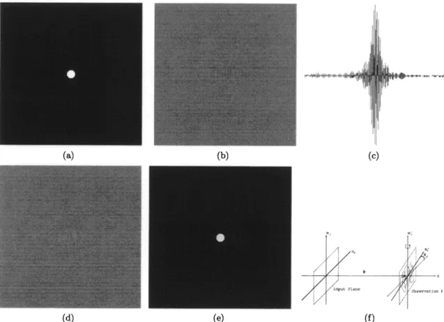
Figure 1. (a) An input object. (b) Real part of the diffraction pattern corresponding to the input pattern, shown in Figure 1(a). (the diffraction pattern is on an observation plane which has a 45° tilt angle around y-axis) (c) The

cross-section taken at the center of real part of the diffraction pattern shown in Figure 1(b). (d) Off-axis hologram of the object shown in Figure 1(a) and calculated on the tilted observation plane given in Figure 1(f). (e) Reconstructed object from off-axis hologram over the tilted plane as shown in Figure 1(d). (f) The implemented scenario.

(c)

(f)

Figure 1. (a) An input object. (b) Real part of the diffraction pattern corresponding to the input pattern, shown in Figure 1(a). (the diffraction pattern is on an observation plane which has a 45° tilt angle around y-axis) (c) The

cross-section taken at the center of real part of the diffraction pattern shown in Figure 1(b). (d) Off-axis hologram of the object shown in Figure 1(a) and calculated on the tilted observation plane given in Figure 1(f). (e) Reconstructed object from off-axis hologram over the tilted plane as shown in Figure 1(d). (f) The implemented scenario.

(6)

4. SIMULATION RESULTS

In the simulation that is presented in this section, the variable N which determines the size of the input and the kernel, is taken as 512. To be precise in the calculations 8 bytes are used to represent the variables. The

simulation results displayed as an image and 256 gray levels are used to represent the field strength. The variable

A is taken as 633mm. The parameters which determine the reference beam R and F are chosen as 200 and 0.8, respectively. During the reconstruction process the DC component is subtracted to decrease the effect of the

uniform beam of light propagating through the hologram. The array fD(n3 ,m3)which represents a simple input

object is shown in Figure 1(a). The spatial sampling is chosen as 2A and the distance between the centers of

the input and the observation planes is taken as 2048A. The tilt angle of observation plane around y-axis is 45°.

There is an illustration of the implemented scenario in Figure 1(f). The real part of the diffraction pattern and

its cross-section on the observation plane are given in Figures 1(b) and 1(c). The figure 1(d) provides the off-axis

hologram of the object on the observation plane. The reconstructed object from the off-axis hologram can be

seen in Figure 1(e).

5. CONCLUSION

The proposed model is based on the Rayleigh-Sommerfeld diffraction integral, and therefore, more accurate than Fresnel or Fraunhofer approximations. Yet the calculation of the diffraction pattern between input and observation planes is still efficient. As a result of using DFT algorithm we can only simulate periodic input and diffraction patterns. Unfortunately, the distortion due to this implicit periodicity, compared to the usually desired non-periodic case, is more dominant at large tilt angles. It is observed that upto 600 degrees of tilt can still be successfully simulated for small objects (such as having size at most f). Moreover,when the distance

is chosen as the distortion in the calculated diffraction pattern is less compared to the cases having larger

distances.

REFERENCES

1. S. Ganci, "Fourier diffraction through a tilted slits," Eur. J. Phys 2, pp. 158—160, 1981.

2. H. Rabal, N. Bolognini, and E. Sicre, "Diffraction by a tilted aperture, coherent and partially coherent

cases," Opt. Acta 32, pp. 1309—1311, 1985.

3. D. Leseberg and C. Frére, "Computer generated holograms of 3D objects composed of tilted planar

seg-ments," Appi. Opt. 27, pp. 3020—3024, 1988.

4. C. Frére and D. Leseberg, "Large objects reconstructed from computer generated holograms," Appi. Opt. 28, pp. 2422—2425, 1989.

5. T. Tommasi and B. Bianco, "Frequency analysis of light diffraction between rotated planes," Opt. Lett. 17,

pp. 556—558, 1992.

6. T. Tommasi and B. Bianco, "Computer-generated holograms of tilted planes by a spatial frequency

ap-proach," J. Opt. Soc. Am. A 10, pp.299—305, 1993.

7. N. Delen and B. Hooker, "Free-space beam propagation between arbitrarily oriented planes based on full

diffraction theory: a fast fourier transform approach," J. Opt. Soc. Am. A 15, pp. 857—867, 1998.

8. K. Matsushima, H. Schimmel, and F. Wyrowski, "Fast calculation method for optical diffraction on tilted

planes by use of the angular spectrum of plane waves," J. Opt. Soc. Am. A 20, pp. 1755—1762, 2003. 9. J. Goodman, Introduction to Fourier Optics, McGrawHill, New York, 1996.

10. G. B. Esmer and L. Onural, "Simulation of scalar_{optical diffraction between arbitrarily oriented planes,"}

in Control, Communications and Signal Processing, 2004. First International Symposium on 2004,

(Ham-mamet, Tunisia), 2004.