Constrained Optimal Hybrid Control
of a Flow Shop System
Kagan Gokbayrak, Member, IEEE, and Omer Selvi
Abstract—We consider an optimal control problem for the hybrid model of a deterministic flow shop system, in which the jobs are processed in the order they arrive at the system. The problem is decomposed into a higher-level discrete-event system control problem of determining the optimal service times, and a set of lower-level classical control problems of determining the optimal control inputs for given service times. We focus on the higher-level problem which is nonconvex and nondifferentiable. The arrival times are known and the decision variables are the ser-vice times that are controllable within constraints. We present an equivalent convex optimization problem with linear constraints. Under some cost assumptions, we show that no waiting is observed on the optimal sample path. This property allows us to simplify the convex optimization problem by eliminating variables and constraints. We also prove, under an additional strict convexity assumption, the uniqueness of the optimal solution and propose two algorithms to decompose the simplified convex optimization problem into a set of smaller convex optimization problems. The effects of the simplification and the decomposition on the solution times are shown on an example problem.
Index Terms—Constrained hybrid control, controllable pro-cessing times, flow shop, hierarchical decomposition, optimal control.
I. INTRODUCTION
W
E consider a deterministic flow shop system consisting of stages that are processing identical jobs. Associ-ated with each job are physical and temporal states. The physical state of a job at stage denoted by describes a measure of quality of the job such as temperature, chemical composition, bacteria level, etc. At each stage , the physical state at time starts out at the initial state and a control input is applied. The physical state is modified to reach the prespecified target state according to the time-driven dynamics described by the differential equations(1) (2) over the time period . If and when the physical state reaches clearly depends on the control input and the physical dynamics (1), (2). We assume that control inputs that can bring the physical state to the target state are avail-able and denote the corresponding service times as . Manuscript received May 15, 2006; revised March 3, 2007. Recommended by Associate Editor J. Hespanha.
The authors are with the Department of Industrial Engineering, Bilkent University, Ankara, 06800 Turkey (e-mail: [email protected]; [email protected]).
Digital Object Identifier 10.1109/TAC.2007.910668
We also assume that the physical states are not altered during the waiting periods; hence, the initial physical states for these identical jobs at each stage are independent of the job index.
A service cost , given as
(3) is associated with the physical process applied on job at stage . Since the final value is prespecified, we do not have an additional cost term for the final state. In order to simplify the analysis, we assume time invariance of the system and drop the term from . Hence, in what follows, the service cost is
denoted by .
The temporal state , on the other hand, keeps the departure time information of job from stage and evolves according to the event-driven dynamics given by the Lindley equation (see [1])
(4) (5) where is the arrival time of job at the system, assumed to be prespecified. A completion-time cost , which is as-sumed to be regular (increasing in ), is incurred for each job departing the system.
In what follows, we consider the minimization of a bicriteria objective function, consisting of service and completion-time costs, subject to physical dynamics (1), (2) and temporal dy-namics (4), (5). Our decision variables are the control inputs that are observed both in physical and temporal dynamics; therefore, the problem considered can be classified as a hy-brid control problem. The hierarchical method, proposed in [2], [3], and [4], allows us to decompose the original hybrid control problem into several lower-level continuous-time optimal con-trol problems and a higher-level discrete-event concon-trol problem of determining the optimal service times. The lower-level prob-lems, rather simple applications of the classical optimal control theory, define service costs that depend only on the processing times, as well as mappings from the processing times to the optimal control inputs. The higher-level problem with service times as the decision variables, on the other hand, is chal-lenging, therefore, attracted attention in the scheduling and the hybrid system control contexts.
In the scheduling literature, sequencing problems with controllable processing times have been considered over the 0018-9286/$25.00 © 2007 IEEE
last three decades. Vickson, in [5], considered the single-machine sequencing problem with the objective of minimizing a total schedule cost consisting of service costs, assumed to be decreasing linear functions of processing times, and weighted completion-time costs. A heuristic algorithm was proposed to determine the optimal job sequence and the corresponding processing times, which are chosen from con-tinuous sets. Chen et al., in [6], considered the single-machine sequencing problem with service costs that are decreasing (not necessarily linear) functions of discrete processing times. It was shown that the problems with total schedule costs consisting of service costs and weighted completion-time or earliness-tardiness-penalty costs can be formulated as assignment problems, hence, can be solved in polynomial time. Similar scheduling problems for parallel machines were considered by Alidaee and Ahmadian in [7] and Cheng et al. in [8]. Alidaee and Ahmadian assumed decreasing linear service costs and formulated the problems as transportation problems that can be solved by polynomial time algorithms. Cheng et al., on the other hand, considered decreasing convex service costs, and formulated the optimization problems as assignment problems, which can also be solved in polynomial time. A survey of results on the controllable processing times can be found in [9] and [10].
The scheduling problems of permutation flow shops are known to be NP-hard even for fixed processing times (see [11]). Therefore, the scheduling literature for multistage systems is limited to heuristics and approximate solution methods. Nowicki in [12], assumed decreasing linear service costs on each machine and provided an approximation algorithm for minimizing the sum of service and weighted makespan costs. In the flow shop scheduling problems, the task of selecting the optimal processing times for a given sequence is viewed as a subproblem, e.g., by Karabati and Kouvelis in [13]. Karabati and Kouvelis considered a scheduling cost, which is a weighted sum of service and cycle time costs for a minimum product set. In their iterative algorithm, the service cost considered is a decreasing linear function of the processing times, so that a linear programming formulation is obtained and solved by a row generation scheme at each iteration.
The related hybrid system control literature, on the other hand, assumes that jobs are served in a given sequence, and concentrates on determining the optimal control inputs, which in turn determine the optimal processing times. Even though this line of research seems to be solving the subproblem in scheduling, an important difference is that the service costs depend on the time-driven dynamics (1), (2); hence, they cannot be assumed to have an arbitrary function form. Moreover, the optimal control inputs for the physical processes are also deter-mined. Pepyne and Cassandras in [14] formulated an optimal control problem for a single-stage manufacturing process and used calculus of variations techniques to obtain structural properties of the optimal solution. The quadratic objective function was designed to complete jobs as fast as possible with the least amount of control effort. In [15], they extended their results to nonregular completion-time costs penalizing earliness and tardiness with given due dates. The uniqueness of the optimal solution of the generalized problem was shown in
[16]. Exploiting the structural properties of the optimal sample path, efficient algorithms were developed in [17], [18], and [19] for solving the higher-level problem for single-stage systems. In these “backward-in-time” and “forward-in-time” algorithms, the original higher-level problem was decomposed into a set of smaller convex optimization problems with linear constraints. In the case of blocking, an efficient algorithm was presented in [20]. Similar models exist for optimal release time (see [21] and [22]) and lot-sizing (see [23]) problems of manufacturing systems.
The application of the hybrid systems framework to multi-stage systems was proposed in [24] where approximate solu-tions for two-stage systems were obtained using the Bezier ap-proximation method to smooth out the max functions in the event-driven dynamics. Earlier work in [25] considered a mul-tistage hybrid system model with constrained service times and presented some optimal sample path characteristics. In [26], we considered two-stage manufacturing systems with no con-straints on the service times and identified some new optimal sample path characteristics to simplify the discrete-event control problem. In particular, we showed that no waiting is observed between stages on the optimal sample path. The transformation of the nonsmooth discrete-event optimal control problem into an equivalent convex optimization problem with linear constraints was also presented in [26], which was then simplified utilizing the no-wait property. In this paper, we combine and extend the results from [18], [25], and [26] for a multistage model with constrained service times. We show that the no-wait property ex-tends to these systems for which simplified convex optimization problems are determined. Under an additional strict convexity assumption, these optimization problems are decomposed by “forward-in-time” algorithms into smaller convex optimization problems with linear constraints.
The rest of the paper is organized as follows. In Sec-tion II, we set up a constrained optimal hybrid control problem and decompose it into several lower-level continuous-time optimal control problems and a higher-level discrete-event optimal control problem. Since the continuous-time optimal control methods are well established, we focus on the dis-crete-event optimal control problem, which is nonconvex and nondifferentiable, therefore, challenging. In this section, we also present a convex optimization problem, which has the same solution as the discrete-event optimal control problem. Section III presents some characteristics of the optimal solu-tion and shows that no waiting is observed between stages on the optimal sample path. The convex optimization problem is, then, simplified employing the no-wait property. Also in Sec-tion III, we give independent period definiSec-tions and present a decoupling property required for the decomposition algo-rithms. Two forward decomposition algorithms are also pre-sented in this section to decompose the simplified convex problem into smaller convex optimization problems with linear constraints. In order to demonstrate the solution method, Sec-tion IV presents an example system, where each job goes through a sequence of linear time invariant processes. Numer-ical results are also given in this section to show the benefits of the simplification and the decomposition in terms of solution times. Finally, Section V concludes the paper.
II. PROBLEMFORMULATION
Let us consider a sequence of identical jobs arriving at an -stage flow shop system at prespecified times
. Servers process one job at a time on a first-come first-served nonpreemptive basis. The service times are con-strained to be , i.e., the process at stage takes at least
amount of time possibly due to bounded inputs .
We consider the optimal hybrid control problem, denoted by , which has the following form:
(6) subject to both time-driven dynamics (1), (2) and event-driven dynamics (4), (5).
Let us now consider the process of job at stage and min-imize its service cost for a given
subject to (1) and (2). This is a classical optimal control problem with state specified at fixed terminal time (see [27]). Let the op-timal control input be denoted as and the optimal ser-vice cost be denoted as where
(7)
subject to (1) and (2). Following the same arguments as in [3], (6) can be reduced to the higher-level discrete-event optimal control problem denoted by
(8)
subject to (4) and (5). Note that the solution to the higher-level problem will then help determine the optimal control inputs
(9)
subject to (1) and (2).
Lower-level solution costs (optimal service costs) and op-timal control inputs can be determined via classical optimal control methods (e.g., see [28]). These methods are well estab-lished and are not the focus of this study. We will, instead, dwell on the higher-level problem . This optimization problem is nonconvex and nondifferentiable over the service times space due to the “max” function in (4).
In this setup, the following assumptions are necessary to make the problem somewhat more tractable while preserving the originality of the problem.
Assumption 1: , for , is continuously dif-ferentiable, monotonically decreasing, and strictly convex.
Assumption 2: , for , is continuously dif-ferentiable, monotonically increasing, and convex.
Note that, for the costs satisfying these assumptions, longer processing times will decrease the service costs, while
in-creasing the departure times; hence, the completion-time costs. This tradeoff is what makes our problem interesting.
Since the service costs in (7) are the optimal costs of the lower-level problems, unlike previous work in scheduling and discrete-event system control literature, they are derived costs: We can select the form of the instantaneous cost function in (3), however, the system dynamics (1), (2) also play a role in determining the service cost . We assume that a faster service comes at the expense of more resources, therefore, is more expensive. For example, in a turning oper-ation, a faster process will increase the tooling costs and will require extra supervision.
The completion-time costs , on the other hand, can be viewed as inventory holding costs. Typically, they are linear functions (e.g., see [29]); however, under a continuously com-pounded interest environment, they can also be strictly convex functions of the system time. Note that a convex cost penalizing tardiness also satisfies Assumption 2. In Section IV, we give an example system with costs that satisfy both assumptions.
As shown in the next section, Assumptions 1 and 2 will suffice for the no-wait property. While proving the uniqueness of the optimal solution, however, we will need strict convexity of the completion-time cost .
A. Equivalent Convex Optimization Problem
Let us determine an equivalent convex optimization problem for the nonconvex and nondifferentiable higher-level problem . We obtain it by replacing the constraints
in (4) by the constraints
resulting with the surrogate convex optimization problem de-fined as
subject to
(10)
for all and .
Since the feasible set of the surrogate optimization problem contains the feasible set of the higher-level optimization problem , its optimal cost is upper bounded by the optimal cost of denoted by , i.e., .
Theorem 1: The optimal solution of satisfies
for all and .
Proof: For a contradiction, assume that the optimal
for some and define
. If we perturb the optimal solution so that is re-placed by , the feasibility will be preserved while the cost variation is given by
By Assumption 1, the process cost is monotonically de-creasing, therefore, which contradicts the optimality assumption. Hence
for all and .
Since the optimal solution of is in the feasible set of , the optimal costs and are equal.
III. CHARACTERISTICS OF THEOPTIMALSOLUTION Applying calculus of variations techniques (see [28]) on the convex optimization problem , we obtain a set of necessary conditions for optimality. Let us start with introducing the La-grangian multipliers , , to form the augmented cost
which will be used in the following lemma.
Lemma 1: The optimal solution must satisfy the fol-lowing conditions.
1) For all and
(11) (12) (13) (14) (15) (16) (17) 2) For and (18) 3) For (19) 4) For (20) 5) (21)
Proof: By Theorem 1, (11) is satisfied. The optimal
so-lution should also satisfy the service constraints (12). From the augmented cost formulation, we obtain the necessary conditions for optimality
(22) (23)
and (14)–(16) for all and . The
con-dition (23) leads to (18)–(21). Finally, from (14), (22), and since by Assumption 1, , we have for all
and
This lemma provides the results needed for the following proofs.
A. Optimality of No-Wait Systems
Let us denote job by , and give definitions of blocks and busy periods needed to decompose the sample path at any stage .
Definition 1: A contiguous set of jobs is said to form a block at stage if:
1) and ;
2) for .
Definition 2: A contiguous set of jobs is said to form a busy period at stage if:
1) and ;
2) for .
Note that busy periods are formed of single or several blocks. Before proceeding with the next lemma, we would like to make a note that its conditions are never satisfied on the optimal sample path. However, this lemma is needed for the contradic-tion argument for proving Theorem 2.
Using Lemma 1, we can show the following monotonicity properties of the optimal service times.
Lemma 2: (Monotonicity properties) If jobs and are in the same block of the th stage on the optimal sample path
then, for and , the optimal
service times satisfy:
i) ;
Proof: We show i) and ii) by contradiction arguments as
follows.
i) Let us assume that jobs and are in the same block of the th stage on the optimal sample path and
. From (12), there are two possible cases.
Case 1) : From (14), and
Case 2) : From (14),
From both cases, for the assumption , we get (24) Since jobs and are in the same block of the th stage on the optimal sample path, we have
(25) From (11), (15), and (25), we have .
For , from (18) and (15)
and for , from (19)
Hence, for
(26) It follows from (13), (24), and (26) that
for and . By
Assump-tion 1, is monotonically increasing; therefore, , which contradicts the initial assump-tion.
ii) Let us assume that jobs and are in the same block of the th stage on the optimal sample path and
. Following the same argument as above, we can write
(27) It follows from (13), (15), (18), and (27), and that
for and . By Assumption
1, is monotonically increasing, therefore , which contradicts the initial
assumption.
The following lemma establishes that, on the optimal sample path, the last job of a busy period does not wait for service in the following stage.
Lemma 3: Consider the job sequence forming
a busy period at stage where on the
optimal sample path. Then, the inequality
is satisfied.
Proof: Let us start with the case where , i.e., jobs are forming the last busy period at stage and assume that . Then, from (11), (15), and (20)
which contradicts (17) in Lemma 1. Hence,
for all .
Next, let us consider the case where . Since is the last job of the busy period at stage
(28) Let us assume that . From (11), (15), (16), and (18)
which also contradicts (17) in Lemma 1. Hence, , if ends a busy period at stage .
The next theorem, which shows that it is never optimal to have buffering between stages, is employed to simplify the convex optimization problem .
Theorem 2: (No-wait property) On the optimal sample path,
the departure times satisfy
for all and .
Proof: (By induction) Let us pick an arbitrary stage
For , we have
Next, let us assume that, for some , the in-equalities
(29) hold for all . We need to show that
also holds so let us assume for a contradiction that the inequality
(30) is satisfied.
Let job end the busy period at stage in which job resides. Note that if , then we already have a contradiction
by Lemma 3, so let us consider the nontrivial case where . We will show by induction that the assumptions (29) and (30) lead to
for all . The inequality will
contradict the result from Lemma 3 concluding the proof. From (30), we can conclude that and are in the same block of stage . Then, from Lemma 2, we have
(31) and
(32) Note that
and from (29)
It follows from (30) that
therefore
(33) From (31)–(33), we obtain
(34) Since we are considering the case where , jobs and reside in the same busy period at stage , therefore
Since jobs and reside in the same block of stage
From (30) and (34), we have
which concludes the basis part of the induction proof. Next, let us assume that the inequalities
(35)
hold for all , where . Since jobs
are in the same block at stage , it follows from Lemma 2 and (34) that
(36)
Since jobs and are in the same busy period at stage
Since, from (35), jobs and are in the same block at stage
Hence, from (35) and (36)
which concludes the inductive step and the induction proof. Since the assumption (30) leads to
which contradicts the result from Lemma 3, we can state that, on the optimal sample path, the departure times satisfy
for all and .
Note that in Theorem 2, the result from Lemma 3 is general-ized to all jobs.
Applying the no-wait property to the higher-level problem , we get subject to (37) (38) (39) (40) for and .
Let us denote the cost incurred by the jobs as
(41)
and define the convex optimization problem
(42)
subject to
(43) (44)
(45) (46) (47)
for and . Following the same
rea-soning as in Theorem 1, we can show that the convex optimiza-tion problem yields the optimal solution for . This simplified convex optimization problem has
decision variables, one equality and inequality constraints (excluding the boundary value constraints). In the next subsection, we give the definition of an independent period structure and present a decoupling property which allows for the decomposition of the simplified problem into smaller convex optimization problems, one for each independent period.
B. Forward Decomposition Algorithms
The decomposition algorithms that follow will require to have a unique optimal solution. A sufficient con-dition for this to be satisfied is given in the next assumption replacing Assumption 2.
Assumption 3: , for , is continuously dif-ferentiable, monotonically increasing, and strictly convex.
Lemma 4: The convex optimization problem has a unique solution.
Proof: The feasible set defined by the constraints (43)–(47)
is convex. Recalling that
(48)
a sufficient condition for to have a unique optimal so-lution is that the cost
is strictly convex.
Let us define two distinct feasible solutions and such that
for , 2. Due to convexity of and (as in Assump-tions 1 and 3), we can write for
For strict inequality (and strict convexity), it suffices to show
that for some and , or .
Since and are distinct, they should differ in at least one component. If for some and , since is strictly convex by Assumption 1, strict inequality is obtained. If, on the other hand, for all and , then for some , we should
have . From (48), it follows that .
Since is strictly convex by Assumption 3, strict inequality is obtained. Hence, for distinct feasible solutions and
i.e., is strictly convex and, therefore, has a unique optimal solution.
In what follows, we determine the unique optimal solution for . Independent period structures, defined next, simplify our task.
Definition 3: A contiguous set of jobs is said to form an independent period for the system if:
1) and for all
;
2) and for all
;
3) for all , or
for some .
Definition 4: An independent period structure for the system
is a partition of jobs into independent periods. The next lemma presents the decoupling property between independent periods.
Lemma 5: Consider a contiguous job sequence
forming an independent period on the optimal sample path. The optimal service times for these jobs do not depend on the arrival
times of the other jobs.
Proof: From (12) and the independent period definition,
we have for all
(49) (50) for and (51) (52) for .
From (11), (16), (18), (51), and (52), for
and
Hence, there is no dependence of for to jobs , i.e., the co-state equations do not propagate information in the backward direction between independent pe-riods. Note that if then there is no need for checking the backward information propagation.
Similarly, let us employ inequalities (49) and (50) in (11) to observe that
Hence, there is no dependence of for to jobs , i.e., the state equations do not propagate infor-mation in the forward direction between independent periods. Note that if then there is no need for checking the for-ward information propagation.
Hence, independent periods are decoupled from each other.
Let us assume that the optimal independent period structure is given. Let be the number of independent periods in this structure, and let and denote the first and the last jobs of the th independent period where . We can rewrite as
subject to (37)–(40). By the independent period definition, the constraints (38)–(40) for can be reduced to
which is satisfied by the optimal solution. Along with the decoupling property shown in Lemma 5, this allows for the decomposition of into smaller optimization problems
defined as
subject to
for and . Note that,
fol-lowing similar reasoning as in Theorem 1, can be shown to have the same optimal solution as of .
We denote the optimal solution of as and , and the corresponding departure times as
for and . The following corollary fol-lows from Lemma 5 and relates the optimal solution of to the optimal solution of the higher-level problem.
Corollary 1: If the job sequence forms an in-dependent period on the optimal sample path, then the optimal solution to satisfies
for and .
This corollary forms the basis for our decomposition algo-rithms.
So far, we have shown that if the optimal independent pe-riod structure can be identified, can be decomposed into a set of smaller problems. The following lemma provides necessary and sufficient conditions for identifying the indepen-dent periods on the optimal sample path based on the solution
of .
Lemma 6: Let initiate an independent period on the op-timal sample path. The job ends the independent period if and only if the following conditions are satisfied:
1) and for
all ;
2) for all , or
for some .
Proof: (Necessity) Since jobs form an independent period on the optimal sample path, and since by Corollary 1, the result follows from the independent period definition.
(Sufficiency) Assume that even though both conditions are satisfied, does not end the independent period, i.e., for some , jobs form an independent period on the optimal sample path.
Let us define a solution for as and otherwise (53) and (54) where is defined as
By the independent period definition, since is not the last job of the independent period, or
for some . It
follows from the first condition that
(55) or
(56)
for some and . Therefore, from
Lemma 4, the solution given in (53) and (54) is not optimal for .
Let us check the feasibility of this nonoptimal solution:
Since and for and are
the solutions for the problem , they satisfy the
con-straints (43)–(47) for and . For
, we have
satisfying the constraints (44) and (45). It follows from the first
condition and from for all that the
constraints (46) and (47) are also satisfied for . Finally,
since and for and are
the solutions for , the constraints (44)–(47) are satisfied
for and . Hence, the nonoptimal
Let us recall from Corollary 1 that
for and , and consider the problem
. Its optimal cost can be written as
(57) where
and
The cost due to applying the nonoptimal solution in (53) and (54) can be written as
(58) where
Since the optimal solution of is unique by Lemma 4, from (55) and (56)
(59) Moreover, due to Assumption 1
(60) which also accounts for the case that . From (57)–(60)
in other words, the cost of the nonoptimal solution is lower than the optimal cost, which is a contradiction. Hence, the result fol-lows.
Lemma 6 allows us to identify independent periods on the optimal sample path. If is the first job of an independent period, we can identify this independent period by sequentially solving and checking for all jobs to see if both conditions in Lemma 6 are satisfied.
The next lemma indicates that checking only for job to see if the first condition in Lemma 6 is satisfied suffices to identify the independent period.
Lemma 7: Let initiate an independent period on the
optimal sample path. For all , if or
for some , then for
all , or
for some .
Proof: (By contradiction) Let us assume that there exists
such that and
for all . In that case job ends an inde-pendent period (not necessarily the one that was started by job ). From the decoupling property in Lemma 5 and Corollary 1, for all stages , we should have
However, since or
for some , a contradiction is observed. Hence, the result follows.
Lemma 7 asserts that an independent period formed by jobs is identified as soon as the problem is solved. This result is formalized in the following theorem.
Theorem 3: Jobs form an independent period on the optimal sample path if and only if the following condi-tions are satisfied:
1) and for all
;
2) for all , or
for some ;
3) and for
all .
Proof: It follows from Lemma 6, Lemma 7, and the
inde-pendent period definition.
Our first forward decomposition algorithm is based on The-orem 3. While identifying the optimal independent period struc-ture, this algorithm also determines the optimal solution.
Algorithm 1:
Step 1: (initialization) , ,
while do
Step 2: solve subproblem
Step 3: (identify independent periods)
if and
for all to then
for and
end if
Step 4: (increment index )
A slightly modified version of this algorithm can be shown to exist. The following theorem forms the basis for this modifica-tion.
Theorem 4: Let jobs form an independent pe-riod on the optimal sample path. If for some ,
and for all
and
for .
Proof: The given solution is formed by the optimal
solu-tions of and . We need to show its feasibility for the problem .
The optimal solutions for , and ,
satisfy (43)–(47) for and .
Since and the solution of satisfies
, the constraints (44) and (45) are satisfied for . Since
and for all , the
con-straints (46) and (47) are also satisfied for . The optimal
solutions for , and ,
sat-isfy (43)–(47) for and . Hence,
the solution in the theorem statement is feasible and optimal. Our second forward decomposition algorithm is based on Theorem 4.
Algorithm 2:
Step 1: (initialization) , ,
while do
Step 2: solve subproblem Step 3:
if and
for all to then
for and
end if
Step 4: (increment index )
Note that these decomposition algorithms require only iter-ations. However, these iterations are not identical in complexity and depend on the arrival sequence along with the cost param-eters. The best case for these algorithms would be an optimal sample path where each job forms an independent period of its own. In this case, for all are solved. The worst case for these algorithms, on the other hand, would be an optimal sample path where all jobs reside in the same inde-pendent period and no decomposition is observed. In the worst case, we solve for all . If the number of independent periods expected are low, e.g., for the bulk arrivals case we have only one independent period, we may choose to solve directly.
We would like to point out that Algorithms 1 and 2 are pretty much the same algorithm, except for the inequality in step 3 which is strict in Algorithm 1 and not strict in Algorithm 2. Due to numerical errors in solutions, we expect both algorithms to work with the same performance.
IV. NUMERICALEXAMPLE
Let us consider an -stage serial manufacturing line pro-cessing an identical set of jobs. Let job at stage have the time-driven dynamics described by
with given initial and final (desired) states. In order to have time-invariant processes at each stage, values are assumed to be constants for . Each stage is assumed to have a bounded control input, i.e., , and to process one job at a time on a first-come first-served nonpreemptive basis. Let , the service cost at stage , be given by the quadratic cost functional defined as
for given . Applying classical optimal control methods, the optimal cost of the lower-level problem for a given service time
can be found as
where
(61) The optimal control input turns out to be constant
(62) for service times where
(63) The departure time cost for job , on the other hand, is given by a cost on its system time defined as
(64) for some constant .
Note that the lower-level optimal cost
is continuously differentiable, monotonically decreasing, and strictly convex satisfying Assumption 1. Similarly the departure
time cost is continuously
differen-tiable, monotonically increasing and strictly convex for , hence, satisfies Assumption 3. Therefore, we ex-pect to see a unique solution as shown in Lemma 4.
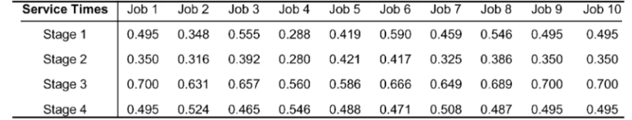
TABLE I OPTIMALSERVICETIMES
TABLE II OPTIMALDEPARTURETIMES
The convex optimization problem we had before the results of Section III can be written as
subject to
for and . This problem has
decision variables, equality constraints, and in-equality constraints (excluding the boundary value constraints on service times). Its solution time will be compared against the solution times of with and without decomposition. The Matlab function fmincon, provided in the Optimization Toolbox, solves these convex optimization problems to opti-mality starting with the same initial solutions. This function implements a sequential quadratic programming (SQP) algo-rithm (see [30] and [31]). The computing environment has an Intel Pentium M 745 processor [1.80 GHz, 2MB L2 cache, 400 MHz FSB] with 512 MB of RAM.
Example 1: For the system described above, let the number
of stages be and the number of identical jobs be . These jobs arrive at prespecified arrival times
. The parameter in (64) is given to be 10, and the parameters , ,
, , and for 1, 2, 3, 4 are given such that from (61) and (63) we get:
• ;
• .
All service times are initially set to be for all
and .
The convex optimization problem is solved in 38.67 s to yield the optimal service times and the optimal departure times, given in Tables I and II, respectively, resulting with an optimal cost of 1290.15. Once the optimal service times are determined, from (62), we can find the optimal control inputs for all jobs and stages .
In , we have decision variables,
equality constraints, and inequality con-straints (excluding the boundary value concon-straints). Note that one may observe the no-wait property, in the optimal solution.
The convex optimization problem , implementing the simplification due to the no-wait property, can be solved in 18.03 s. It has fewer decision variables and constraints: only
decision variables, one equality and inequality constraints (excluding the boundary value constraints); hence, such an improvement in speed is ob-served.
In order to illustrate the speed improvement due to de-composition, we solve the same problem using Algorithm 2. (Algorithm 1 has the same performance for this problem). It decomposes the problem into a set of subproblems for jobs
, , , , , and ,
and yields the optimal solution in only 1.84 s.
Note that the additional improvement observed in the ex-ample due to the decomposition algorithm is not typical. For congested systems, the decomposition algorithms may take longer to yield the optimal solution. For uncongested systems where the number of jobs and stages are large, however, we ex-pect orders of magnitude improvements due to decomposition. The speed improvement due to employing the no-wait property, on the other hand, is always observed regardless of the system load as it decreases the number of variables and constraints considerably.
V. CONCLUSION
This paper considered a deterministic flow shop system with some physical dynamics at each stage. For prespecified arrival times, the hybrid control problem was reduced to a discrete-event control problem where the control variables are the deterministic service times that are lower-bounded. The original nonsmooth optimization problem was transformed into a convex optimization problem over a larger set with linear constraints. We derived some characteristics of the optimal solution and showed that no waiting between stages is observed on the optimal sample path. The no-wait property eliminates N variables and N constraints from the convex optimization problem at each stage it is observed. Two “forward-in-time” decomposition algorithms were also developed to decompose the simplified convex optimization problem into smaller convex optimization problems. As shown by the numerical example, the simplification on the convex optimization problem and the decomposition improved the solution times considerably.
REFERENCES
[1] C. G. Cassandras and S. Lafortune, Introduction to Discrete Event
Sys-tems. Norwell, MA: Kluwer, 1999.
[2] K. Gokbayrak and C. G. Cassandras, “Hybrid controllers for hierar-chically decomposed systems,” in Proc. Hybrid System Control Conf., 2000, pp. 117–129.
[3] K. Gokbayrak and C. G. Cassandras, “A hierarchical decomposition method for optimal control of hybrid systems,” in Proc. 39th IEEE
Conf. Decision and Control, 2000, pp. 1816–1821.
[4] C. G. Cassandras and K. Gokbayrak, “Optimal control for discrete event and hybrid systems,” Model., Control, Optim. Complex Syst., pp. 285–304, 2002.
[5] R. G. Vickson, “Choosing the job sequence and processing times to minimize processing plus flow cost on a single machine,” Oper, Res,, vol. 28, no. 5, pp. 1155–1167, 1980.
[6] Z. L. Chen, Q. Lu, and G. Tang, “Single machine scheduling with dis-cretely controllable processing times,” Oper. Res. Lett., vol. 21, pp. 69–76, 1997.
[7] B. Alidaee and A. Ahmadian, “Two parallel machine sequencing prob-lems involving controllable job processing times,” Eur. J. Oper. Res., vol. 70, pp. 335–341, 1993.
[8] T. C. E. Cheng, Z. L. Chen, and L. Chung-Lun, “Parallel-machine scheduling with controllable processing times,” IIE Trans., vol. 28, no. 2, pp. 177–180, 1996.
[9] E. Nowicki and S. Zdrzalka, “A survey of results for sequencing prob-lems with controllable processing times,” Discrete Appl. Math., vol. 26, pp. 271–287, 1990.
[10] H. Hoogeveen, “Multicriteria scheduling,” Eur. J. Oper. Res., vol. 167, pp. 592–623, 2005.
[11] M. Pinedo, Scheduling: Theory, Algorithms, and Systems, 2nd ed. Englewood Cliffs, NJ: Prentice-Hall, 2002.
[12] E. Nowicki, “An approximation algorithm for the m-machine permuta-tion flow shop scheduling problem with controllable processing times,”
Eur. J. Oper. Res., vol. 70, pp. 342–349, 1993.
[13] S. Karabati and P. Kouvelis, “Flow-line scheduling problem with con-trollable processing times,” IIE Trans., vol. 29, no. 1, pp. 1–14, 1997. [14] D. L. Pepyne and C. G. Cassandras, “Modeling, analysis, and optimal
control of a class of hybrid systems,” J. Discrete Event Dyn. Syst.:
Theory Appl., vol. 8, no. 2, pp. 175–201, 1998.
[15] D. L. Pepyne and C. G. Cassandras, “Optimal control of hybrid sys-tems in manufacturing,” Proc. IEEE, vol. 88, no. 7, pp. 1108–1123, Jul. 2000.
[16] C. G. Cassandras, D. L. Pepyne, and Y. Wardi, “Optimal control of a class of hybrid systems,” IEEE Trans. Autom. Control, vol. 46, no. 3, pp. 398–415, Mar. 2001.
[17] Y. Wardi, C. G. Cassandras, and D. L. Pepyne, “A backward algorithm for computing optimal controls for single-stage hybrid manufacturing systems,” Int. J. Prod. Res., vol. 39-2, pp. 369–393, 2001.
[18] Y. C. Cho, C. G. Cassandras, and D. L. Pepyne, “Forward decomposi-tion algorithms for optimal control of a class of hybrid systems,” Int. J.
Robust Nonlin. Control, vol. 11, pp. 497–513, 2001.
[19] P. Zhang and C. G. Cassandras, “An improved forward algorithm for optimal control of a class of hybrid systems,” IEEE Trans. Autom.
Con-trol, vol. 47, no. 10, pp. 1735–1739, Oct. 2002.
[20] J. Moon and Y. Wardi, “Optimal control of processing times in single-stage discrete event dynamic systems with blocking,” IEEE
Trans. Autom. Control, vol. 50, no. 6, pp. 880–884, Jun. 2005.
[21] M. Gazarik and Y. Wardi, “Optimal release times in a single server: An optimal control perspective,” IEEE Trans. Autom. Control, vol. 43, no. 7, pp. 998–1002, Jul. 1998.
[22] J. Moon and Y. Wardi, “Optimal release times in a single-stage manu-facturing system with blocking: Optimal control perspective,” J. Optim.
Theory Appl., vol. 125, no. 3, pp. 653–672, 2005.
[23] A. D. Febbraro, R. Minciardi, and S. Sacone, “Optimal control laws for lot-sizing and timing of jobs on a single production facility,” IEEE
Trans. Autom. Control, vol. 47, no. 10, pp. 1613–1623, Oct. 2002.
[24] C. G. Cassandras, Q. Liu, D. L. Pepyne, and K. Gokbayrak, “Optimal control of a two-stage hybrid manufacturing system model,” in Proc.
38th IEEE Conf. Decision and Control, 1999, pp. 450–455.
[25] K. Gokbayrak and C. G. Cassandras, “Constrained optimal control for multistage hybrid manufacturing system models,” presented at the 8th IEEE Mediterranean Conf. New Directions in Control and Automation, 2000.
[26] K. Gokbayrak and O. Selvi, “Optimal hybrid control of a two-stage manufacturing system,” presented at the ACC, 2006.
[27] A. E. Bryson and Y. C. Ho, Applied Optimal Control. Bristol, PA: Hemisphere, 1975.
[28] D. E. Kirk, Optimal Control Theory. Englewood Cliffs, NJ: Prentice-Hall, 1970.
[29] E. A. Silver, D. F. Pyke, and R. Peterson, Inventory Management and
Production Planning and Scheduling. New York: Wiley, 1998. [30] P. E. Gill, W. Murray, and M. H. Wright, Practical Optimization.
New York: Academic, 1981.
[31] R. Fletcher, Practical Methods of Optimization. New York: Wiley, 1987.
Kagan Gokbayrak (M’06) was born in Istanbul,
Turkey, in 1972. He received the B.S. degrees in mathematics and in electrical engineering from Bogazici University, Istanbul, the M.S. degree in electrical and computer engineering from the Uni-versity of Massachusetts, Amherst, and the Ph.D. degree in manufacturing engineering from Boston University, Boston, MA, in 1995, 1995, 1997, and 2001, respectively.
From 2001 to 2003, he was a Network Planning Engineer at Genuity, Inc., Burlington, MA. Since 2003, he has been a faculty member in the Industrial Engineering Department of Bilkent University, Ankara, Turkey. He specializes in the areas of discrete-event and hybrid systems, stochastic optimization, and computer simulation, with applications to inventory and manufacturing systems.
Omer Selvi was born in Nigde, Turkey, in 1976. He
received the B.S. and M.S. degrees in industrial en-gineering from Bilkent University, Ankara, Turkey, in 1999 and 2002, where he is currently pursuing the Ph.D. degree.
His research interests are in the fields of discrete-event systems and stochastic optimization.