Acoustical performance analysis of Bilkent University amphitheater "Odeon"

(1)

To the memory of my grandfather Ömer Eken

(2)

ACOUSTICAL PERFORMANCE ANALYSIS

OF

BİLKENT UNIVERSITY AMPHITHEATER “ODEON”

A THESIS

SUBMITTED TO THE DEPARTMENT OF

INTERIOR ARCHITECTURE AND ENVIRONMENTAL DESIGN

AND THE INSTITUTE OF FINE ARTS

OF BİLKENT UNIVERSITY

IN PARTIAL FULFILLMENT OF THE REQUIREMENTS

FOR THE DEGREE OF

MASTER OF FINE ARTS

By

Zühre Sü

May, 2004

(3)

I certify that I have read this thesis and that in my opinion it is fully adequate, in scope and in quality, as a thesis for the degree of Master of Fine Arts.

______________________________________________ Dr. Semiha Yılmazer (Principal Advisor)

______________________________________________ Prof. Dr. Mehmet Çalışkan

______________________________________________ Assoc. Prof. Dr. Cengiz Yener

Approved by the Institute of Fine Arts

____________________________________________________________________ Prof. Dr. Bülent Özgüç, Director of the Institute of Fine Arts

(4)

ABSTRACT

ACOUSTICAL PERFORMANCE ANALYSIS

OF

BİLKENT UNIVERSITY AMPHITHEATER “ODEON”

Zühre Sü

M.F.A. in Interior Architecture and Environmental Design Supervisor: Dr. Semiha Yılmazer

May, 2004

The aim of this study is analyzing the acoustical quality of Bilkent University Amphitheater ODEON by means of assessing the fundamental acoustical parameters for both speech and music. Defining the problems, specifying the causes of the problems and providing a foundation for the ongoing suggestions are within the frame of the analysis. The parameters such as reverberation time, early decay time, clarity, definition, lateral fraction, sound pressure level and sound transmission index are calculated by the computer simulation technique for their assessment to be carried out. Initially, the results of the simulation software are compared with the previous real-size measurements of Bilkent ODEON for the unoccupied condition of the amphitheater, in order to ensure the accuracy of the software. Proving to be a valid tool, the software namely ODEON Room Acoustics Program, is used in the calculations for the occupied condition of the amphitheater as a basis of the study. The results are evaluated from the acoustical design standpoint of a multipurpose hall, which are followed by the suggestions for the improvement of the existing acoustical performance of the amphitheater. Finally, the suggestions are supported through the simulation results of the new hall that is acoustically renovated.

Keywords: Room Acoustics, Acoustical Design, Multipurpose Auditoria, Echo, Reverberation Control, Acoustical Parameters, Acoustical Simulation, Amphitheater

(5)

ÖZET

BİLKENT ÜNİVERSİTESİ AMFİTİYATROSU ODEON’UN

AKUSTİK PERFORMANS ANALİZİ

Zühre Sü

İç Mimarlık ve Çevre Tasarımı Bölümü Yüksek Lisans

Tez Yöneticisi: Dr. Semiha Yılmazer Mayıs, 2004

Bu çalışmanın amacı, konuşma ve müzik ile ilgili akustik parametreleri göz önüne alarak Bilkent Üniversitesi Amfitiyatrosu ODEON’un akustik performans analizini yapmaktır. Analiz kapsamında problemlerin tanımlanması, problemlerin sebeplerinin belirlenmesi ve getirilecek öneriler için temel oluşturulması hedeflenmiştir. Değerlendirmelerin yapılabilmesi için çınlama süresi, erken sönümleme süresi, berraklık, tanımlama, yan yansıma oranı, ses basınç düzeyi ve konuşma iletim indisi gibi parametreler bilgisayar benzetim tekniğiyle hesaplanmıştır. İlk olarak benzetim programının doğruluğunu belirlemek amacıyla, amfitiyatronun boş konumu için benzetim sonuçları Bilkent ODEON’da daha önceden yapılmış gerçek ölçümler ile kıyaslanmıştır. Geçerliliğinin kanıtlanmasıyla, ODEON Room Acoustics Program isimli benzetim programı, çalışmanın temelini oluşturan amfitiyatronun dolu konumu için yapılan hesaplamalarda kullanılmıştır. Sonuçlar çok amaçlı salonların akustik tasarım kriterleri baz alınarak değerlendirilmiştir. Değerlendirmeleri takiben, salonun şu anki akustik performansını iyileştirmek için bir takım öneriler getirilmiştir. Son olarak, getirilen bu öneriler salonun akustik açıdan iyileştirilmiş yeni haliyle yapılan benzetim sonuçları ile desteklenmiştir.

Anahtar Kelimeler: Oda Akustiği, Akustik Tasarım, Çok Amaçlı Oditoryum, Eko, Çınlama Süresi Kontrolü, Akustik Parametreler, Akustik Benzetim, Amfitiyatro

(6)

ACKNOWLEDGMENTS

First and foremost, I would like to express sincere appreciation to my supervisor Dr. Semiha Yılmazer, for her friendly guidance, encouragement and patience. Without her positive energy and fresh mind, I would hardly succeed in the formation of this study and find a route for my research. It is also my duty to express deepest gratitude to Prof. Dr. Mehmet Çalışkan, for his generous help and tutorship. I could not have completed this study without his technical support and invaluable suggestions.

I would also like to thank to Assoc. Prof. Dr. Cengiz Yener and Prof. Dr. Mustafa Pultar, for their remarkable contribution to my graduate education. I am grateful to Ramiz Akgün and Erkut Şahinbaş, for giving me encouragement in this study and for their support in reaching the necessary documents.

Special thanks to all of my friends for their continuous support of friendship. Lastly, but not least, my greatest indebtedness is to my family to whom I owe what I have -Ömer Eken, Zuhal Eken, İsmail Sü, Kamile Eken, Reha Eken and Şaban Taşgın- for their trust and support in every aspect of my life, and particularly to Emine Taşgın for her endless love, presence and guidance through all the steps of my life.

(7)

2. ACOUSTICAL REQUIREMENTS IN AUDITORIUM DESIGN 5 2.1. Subjective Criteria ... 6 2.1.1. Intimacy... 6 2.1.2. Warmth ... 7 2.1.3. Loudness ... 8 2.1.4. Envelopment ... 9 2.1.5. Reverberance... 9 2.1.6. Subjective Clarity... 10 2.1.7. Diffusion ... 11 2.2. Objective Criteria ... 12 2.2.1. Reverberation Time (RT) ... 12

2.2.2. Early Decay Time (EDT) ... 15

2.2.3. Clarity (C80) ... 16

2.2.4. Definition (D50)... 18

2.2.5. Lateral Fraction (LF)... 19

2.2.6. Strength (G)... 20

2.2.7. Initial-Time-Delay Gap (ITDG)... 21

2.3. The Nature of Speech and Music Sounds ... 22

2.3.1. Acoustics for Speech ... 24

2.3.1.1. Speech Intelligibility... 25

2.3.1.2. Speech Transmission Index (STI) ... 27

2.3.2. Acoustics for Music ... 28

2.3.3. Meeting the Requirements of both Speech and Music... 30

2.3.4. Acoustical Defects ... 35

2.3.4.1. Echo ... 36

2.3.4.2. Sound Foci ... 39

2.3.4.3. Sound Masking ... 41

2.3.4.4. Coloration and Distortion of Timbre ... 42

3. BİLKENT ODEON 44 3.1. Architecture, Shape and Size ... 45

(8)

4. REAL-SIZE MEASUREMENTS AT BİLKENT ODEON 51

4.1. Equipment, Method and Input Data ... 52

4.2. Measurement and Evaluation of the Results ... 56

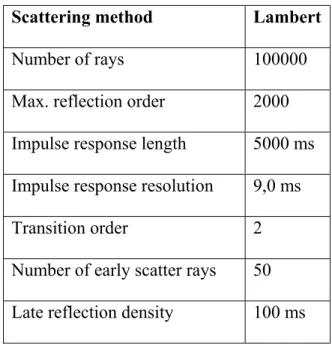
5. COMPUTER SIMULATION OF BİLKENT ODEON 70 5.1.Method and the Input Data for the Simulation ... 72

5.2.Comparison of the Computer Simulation with the Real-Size Measurements... 80

5.2.1. Reverberation Time (T30) Distribution Maps ... 86

5.2.2. Early Decay Time (EDT) Distribution Maps... 87

5.2.3. Clarity (C80) Distribution Maps ... 88

5.2.4. Definition (D50) Distribution Maps... 89

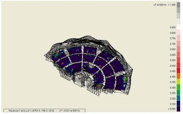
5.2.5. Lateral Fraction (LF) Distribution Maps ... 90

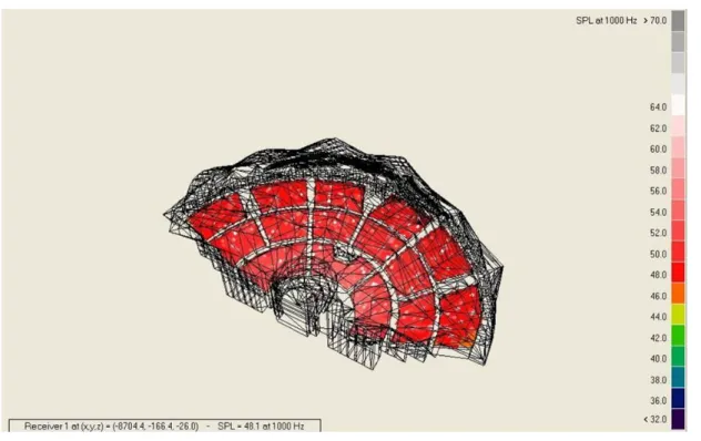
5.2.6. Sound Pressure Level (SPL) Distribution Maps ... 91

5.2.7. Sound Transmission Index (STI) Distribution Maps ... 92

5.3. Simulation of the Hall for the Fully-Occupied Condition... 98

5.3.1. Reverberation Time (T30) Distribution Maps and Graphs .... 103

5.3.2. Early Decay Time (EDT) Distribution Maps and Graphs ... 106

5.3.3. Clarity (C80) Distribution Maps and Graphs... 109

5.3.4. Definition (D50) Distribution Maps and Graphs ... 112

5.3.5. Lateral Fraction (LF) distribution Maps and Graphs ... 115

5.3.6. Sound Pressure Level (SPL) Distribution Maps and Graphs. 118 5.3.7. Sound Transmission Index Distribution Maps and Graphs ... 121

5.3.8. Analysis of the Results... 128

6. ACOUSTICAL RENOVATION OF THE HALL 136 6.1. Suggestions for Improvements ... 136

6.2. Simulation of the Acoustical Renovation... 143

6.2.1. Reverberation Time (T30) Distribution Maps and Graphs .... 149

6.2.2. Early Decay Time (EDT) Distribution Maps and Graphs ... 151

6.2.3. Clarity (C80) Distribution Maps and Graphs... 153

6.2.4. Definition (D50) Distribution Maps and Graphs ... 155

6.2.5. Lateral Fraction (LF) Distribution Maps and Graphs ... 157

6.2.6. Sound Pressure Level (SPL) Distribution Maps and Graphs. 159 6.2.7. Sound Transmission Index (STI) Distribution Maps and Graphs... 161

7. CONCLUSION 165

REFERENCES 169 APPENDIX A ARCHITECTURAL DRAWINGS OF BİLKENT ODEON 172

(9)

LIST OF TABLES

Table 1. Objective measures corresponding to subjective attributes ... 5 Table 2. Optimum values of C80 for front and back rows of a hall ... 18 Table 3. Optimum ranges for objective parameters for music use... 22 Table 4. Relation between scores of speech transmission quality and STI

(RASTI) ... 27 Table 5. Some features which distinguish the acoustical design of concert

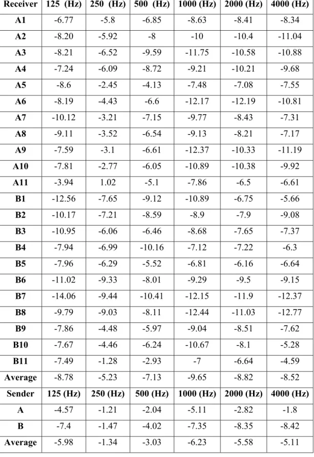
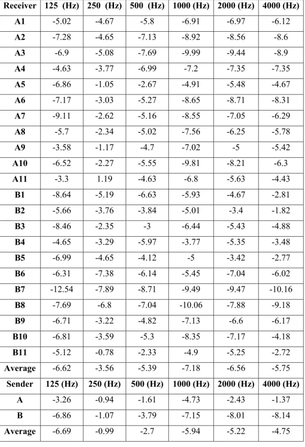
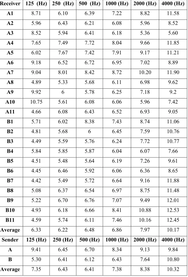
halls, opera houses and drama theaters... 31 Table 6. Optimum values for performance spaces ... 32 Table 7. Measurement coordinates for sender and receiver locations ... 54 Table 8. Measurement results for C50 for the frequency range from 125 to

4000 Hz ... 57 Table 9. Measurement results for C80 for the frequency range from 125 to

4000 Hz ... 58 Table 10. Measurement results for D50 for the frequency range from 125 to

4000 Hz ... 59 Table 11. Measurement results for EDT for the frequency range from 125 to

4000 Hz ... 60 Table 12. Measurement results for RT for the frequency range from 125 to

4000 Hz ... 61 Table 13. Room information for the amphitheater that is taken from the

simulation software ... 74 Table 14. Sound absorption coefficients of different materials used in the

design of ODEON amphitheater ... 79 Table 15. Calculation parameters of the model that are applied in the

Simulation... 79 Table 16. Sound absorption coefficients for new materials used in the

(10)

LIST OF FIGURES

Figure 1. Reverberation time definition with a sample decay ... 13

Figure 2. Optimum reverberation times for different activities ... 15

Figure 3. Impulse response illustrating initial time delay gap ... 21

Figure 4. Sound rays in rooms ... 35

Figure 5. Impulse response with an echo ... 37

Figure 6. Acceptable echo levels for speech under reverberant conditions... 38

Figure 7. Reflection from a concave and a convex surface ... 39

Figure 8. Illustrations of the concave mirror laws ... 40

Figure 9. Methods for avoiding focusing... 41

Figure 10. A partial consonant sound masking by a preceding vowel... 42

Figure 11. Bilkent ODEON perspective view 1 from outside ... 44

Figure 12. Bilkent ODEON perspective view 2 from outside ... 45

Figure 13. Bilkent ODEON the interpretation of travertine cladding with steel frame structure ... 46

Figure 14. Bilkent ODEON front view ... 46

Figure 15. Bilkent ODEON interior view 1 ... 47

Figure 16. Bilkent ODEON interior view 2 ... 48

Figure 17. Bilkent ODEON acoustical bridges ... 50

Figure 18. Selected source and receiver locations ... 55

Figure 19. C50 and C80 values for frequencies from 125 to 4000 Hz ... 62

Figure 20. RT and EDT values for frequencies from 125 to 4000 Hz... 62

Figure 21. 3d color display of ODEON amphitheater view 1... 73

Figure 24. Plan view of the source and receiver locations... 75

Figure 25. Elevation view of the source and receiver locations ... 75

Figure 26. 3d view of the source and receiver location . ... 76

Figure 27. Estimated reverberation times of quick estimate for unoccupied hall ... 81

Figure 28. Material overview for unoccupied hall ... 81

Figure 29. Unused absorption graph for unoccupied hall ... 82

Figure 30. Energy curves for unoccupied hall ... 83

Figure 31. Estimated reverberation times of global estimate for unoccupied hall ... 84

Figure 32. Free path distribution graph for unoccupied hall... 84

Figure 33. Reverberation time distribution map for 500 Hz and for the unoccupied hall ... 86

Figure 34. Reverberation time distribution map for 1000 Hz and for the unoccupied hall ... 86

(11)

Figure 35. Early decay time distribution map for 500 Hz and for the

unoccupied hall ... 87

Figure 36. Early decay time distribution map for 1000 Hz and for the unoccupied hall ... 87

Figure 37. Clarity distribution map for 500 Hz and for the unoccupied hall ... 88

Figure 38. Clarity distribution map for 1000 Hz and for the unoccupied hall .... 88

Figure 39. Definition distribution map for 500 Hz and for the unoccupied hall . 89 Figure 40. Definition distribution map for 1000 Hz and for the unoccupied hall... 89

Figure 41. Lateral fraction distribution map for 500 Hz and for the unoccupied hall... 90

Figure 42. Lateral fraction distribution map for 1000 Hz and for the unoccupied hall ... 90

Figure 43. Sound pressure level distribution map for 500 Hz and for the unoccupied hall ... 91

Figure 44. Sound pressure level distribution map for 1000 Hz and for the unoccupied hall ... 91

Figure 45. Sound transmission index distribution map for the unoccupied hall.. 92

Figure 46. Reverberation times for the selected receiver point in different frequencies ... 98

Figure 47. Energy parameters98 Figure 48. Estimated reverberation times of quick estimate for fully-occupied hall... 99

Figure 49. Material overview for the fully-occupied hall... 99

Figure 50. Unused absorption graph for the fully-occupied hall ... 100

Figure 51. Energy curves for fully-occupied hall ... 101

Figure 52. Estimated reverberation times of global estimate for fully-occupied hall... 101

Figure 53. Free path distribution graph for fully-occupied hall... 101

Figure 54. Reverberation time distribution map for 500 Hz and for the fully-occupied hall ... 103

Figure 55. Reverberation time distribution map for 1000 Hz and for the fully- occupied hall ... 104

Figure 56. Reverberation time cumulative distribution graph for 500 Hz and for the fully-occupied hall... 105

Figure 57. Reverberation time cumulative distribution graph for 1000 Hz and for the fully-occupied hall ... 105

Figure 58. Early decay time distribution map for 500 Hz and for the fully- occupied hall ... 106

Figure 59. Early decay time distribution map for 1000 Hz and for the fully- occupied hall ... 107

Figure 60. Early decay time cumulative distribution graph for 500 Hz and for the fully-occupied hall... 108

Figure 61. Early decay time cumulative distribution graph for 1000 Hz and for the fully-occupied hall... 108

Figure 62. Clarity distribution map for 500 Hz and for the fully-occupied hall . 109 Figure 63. Clarity distribution map for 1000 Hz and for the fully-occupied hall... 110

(12)

Figure 64. Clarity cumulative distribution graph for 500 Hz and for the

fully-occupied hall ... 111

Figure 65. Clarity cumulative distribution graph for 1000 Hz and for the fully-occupied hall ... 111

Figure 66. Definition distribution map for 500 Hz and for the fully-occupied hall... 112

Figure 67. Definition distribution map for 1000 Hz and for the fully-occupied hall... 113

Figure 68. Definition cumulative distribution graph for 500 Hz and for the fully-occupied hall ... 114

Figure 69. Definition cumulative distribution graph for 1000 Hz and for the fully-occupied hall ... 114

Figure 70. Lateral fraction distribution map for 500 Hz and for the fully- occupied hall ... 115

Figure 71. Lateral fraction distribution map for 1000 Hz and for the fully- occupied hall ... 116

Figure 72. Lateral fraction cumulative distribution graph for 500 Hz and for the fully-occupied hall... 117

Figure 73. Lateral fraction cumulative distribution graph for 1000 Hz and for the fully-occupied hall... 117

Figure 74. Sound pressure level distribution map for 500 Hz and for the fully- occupied hall ... 118

Figure 75. Sound pressure level distribution map for 1000 Hz and for the fully- occupied hall ... 119

Figure 76. Sound pressure level cumulative distribution graph for 500 Hz and for the fully-occupied hall ... 120

Figure 77. Sound pressure level cumulative distribution graph for 1000 Hz and for the fully-occupied hall ... 120

Figure 78. Sound transmission index (STI) distribution map for the fully- occupied hall ... 121

Figure 79. Sound transmission index (STI) cumulative distribution graph for the fully-occupied hall... 122

Figure 80. Reflector coverage view 1 ... 126

Figure 83. Plan view for the renovated hall ... 137

Figure 84. Side view for the renovated hall ... 138

Figure 85. The axonometric view for the renovated canopy ... 141

Figure 86. Partial axonometric view of the fragmented beam ... 142

Figure 87. Partial plan view from the fragmented beam surface ... 142

Figure 88. 3d color display of renovated hall view 1... 143

Figure 89. 3d color display of renovated hall view 2... 143

Figure 90. Material overview for the renovated hall ... 145

Figure 91. Energy curves for the renovated hall ... 146

Figure 92. Estimated reverberation times of global estimate for the renovated hall... 147

Figure 93. Free path distribution graph for the renovated hall ... 148

Figure 94. Reverberation time distribution map for 500 Hz and for the renovated hall ... 149

(13)

Figure 95. Reverberation time distribution map for 1000 Hz and for the

renovated hall ... 149

Figure 96. Reverberation time distribution graph for 500 Hz and for the renovated hall ... 150

Figure 97. Reverberation time cumulative distribution graph for 1000 Hz and for the renovated hall ... 150

Figure 98. Early decay time distribution map for 500 Hz and for the renovated hall ... 151

Figure 99. Early decay time distribution map for 1000 Hz and for the renovated hall... 151

Figure 100. Early decay time cumulative distribution graph for 500 Hz and for the renovated hall ... 152

Figure 101. Early decay time cumulative distribution graph for 1000 Hz and for the renovated hall... 152

Figure 102. Clarity distribution map for 500 Hz and for the renovated hall ... 153

Figure 103. Clarity distribution map for 1000 Hz and for the renovated hall ... 153

Figure 104. Clarity cumulative distribution graph for 500 Hz and for the renovated hall... 154

Figure 105. Clarity cumulative distribution graph for 1000 Hz and for the renovated hall... 154

Figure 106. Definition distribution map for 500 Hz and for the renovated hall .. 155

Figure 107. Definition distribution map for 1000 Hz and for the renovated hall. 155 Figure 108. Definition cumulative distribution graph for 500 Hz and for the renovated hall... 156

Figure 109. Definition cumulative distribution graph for 1000 Hz and for the renovated hall... 156

Figure 110. Lateral fraction distribution map for 500 Hz and for the renovated hall ... 157

Figure 111. Lateral fraction distribution map for 1000 Hz and for the renovated hall ... 157

Figure 112. Lateral fraction cumulative distribution graph for 500 Hz and for the renovated hall... 158

Figure 113. Lateral fraction cumulative distribution graph for 1000 Hz and for the renovated hall... 158

Figure 114. Sound pressure level distribution map for 500 Hz and for the renovated hall... 159

Figure 115. Sound pressure level distribution map for 1000 Hz and for the renovated hall... 159

Figure 116. Sound pressure level cumulative distribution graph for 500 Hz and for the renovated hall ... 160

Figure 117. Sound pressure level cumulative distribution graph for 1000 Hz and for the renovated hall ... 160

Figure 118. Sound transmission index distribution map for 500 Hz and for the renovated hall... 161

Figure 119. Sound transmission index cumulative distribution graph for the renovated hall... 161

Figure 120. Reflector coverage view 1 for the renovated hall... 164

Figure 121. Site plan of Bilkent ODEON ... 173

(14)

Figure 123. First floor plan of Bilkent ODEON ... 175

Figure 124. Second floor plan of Bilkent ODEON ... 176

Figure 125. Third floor plan of Bilkent ODEON ... 177

Figure 126. Steel truss construction plan of Bilkent ODEON ... 178

Figure 127. Plan view of the roof membrane of Bilkent ODEON... 179

Figure 128. East elevation of Bilkent ODEON ... 180

Figure 129. South elevation of Bilkent ODEON ... 180

Figure 130. North elevation of Bilkent ODEON ... 180

Figure 131. Section A-A of Bilkent ODEON ... 181

Figure 132. Section B-B of Bilkent ODEON ... 181

Figure 133. Section C-C of Bilkent ODEON ... 181

Figure 134. Magnitude frequency response graph for the receiver location A1.. 183

Figure 135. Schroeder curve for the receiver location A1 ... 183

Figure 136. Energy-time curve for the receiver location A1 ... 183

Figure 137. Group delay graph for the receiver location A1 ... 183

Figure 138. Cumulative spectral decay graph for the receiver location A1... 183

Figure 140. Schroeder curve for the receiver location A2... 184

Figure 143. Cumulative spectral decay graph for the receiver location A2 ... 184

(15)

Figure 175. Schroeder curve for the receiver location A9... 191

Figure 179. Magnitude frequency response graph for the receiver location A10... 192

Figure 184. Magnitude frequency response graph for the receiver location A11 ... 193

Figure 189. Magnitude frequency response graph for the receiver location B1.. 194

Figure 190. Schroeder curve for the receiver location B1 ... 194

Figure 191. Energy-time curve for the receiver location B1 ... 194

Figure 192. Group delay graph for the receiver location B1 ... 194

Figure 193. Cumulative spectral decay graph for the receiver location B1 ... 194

(16)

Figure 234. Magnitude frequency response graph for the receiver location B10 ... 203

Figure 239. Magnitude frequency response graph for the receiver location B11 ... 204

(17)

NOMENCLATURE

C50, C80 (Clarity): The ratio of early sound energy to late sound energy arriving within 80 ms of direct sound to late or reverberant sound energy arriving later than 80 ms after the direct sound.

D50 (Definition): The ratio of the effective energy, which is the direct sound energy and the energy of reflections delayed with respect to the direct sound up to 50 ms, to the total energy in an impulse response.

EDT (Early decay time): The measure of the rate of a sound decay based on measuring the first 10 dB portion of the decay and multiplying it by 6 for corresponding with RT values.

G (Strength): The assessment of the total sound level at a closed volume, for a specific source and receiver configuration, by the comparison of the impulse response energy at this volume with the direct sound level at 10 m for the same source in an open field.

ITDG (Initial-time-delay gap): The time lapse at a listener’s ears between the arrival of the direct sound and the first reflected sound of sufficient loudness.

LF (Lateral fraction): The fraction of lateral energy arriving between 5 and 80 ms after the arrival of direct sound compared to the total sound energy arriving at the listener within the first 80 ms of direct sound arrival.

RT, T30 (Reverberation time): The time required after stopping a sound source for the average sound energy density to decay by 60 dB from an equilibrium level.

SPL (Sound pressure level): The relative quantity, which is the ratio between the actual sound pressure and a fixed reference pressure, used in measuring the magnitude of sound.

STI (Speech transmission index): The single-number rating of transmission loss performance for a construction element tested over a standard frequency range.

(18)

1. INTRODUCTION

1.1. General

One of the main goals of architectural acoustics in the case of multi-purpose auditorium, which is the gathering place for speech and music performances, is to provide both the optimum speech intelligibility and the sound quality. The greatest challenge that the designer confronts at this point is to accommodate both unamplified music and unassisted speech within the same place, which is especially much difficult for the halls with seating capacities exceeding 2000. As it is known that good acoustics for speech and music are generally incompatible, either a compromise in between could be accepted or an electro-acoustical sound reinforcement system should be assisted.

At the earlier stages in the development of architectural acoustics, for the assessment of acoustical performances, the acoustical design of an auditorium was mainly focused on providing an optimum reverberation time. However, further technical developments and experiences of people have shown that it is not sufficient to consider only reverberation time. The acceptance of the limitation of reverberation time encouraged the development of new local criteria of acoustical quality, which were developed in studies of the correlations between objective acoustical parameters and subjective evaluations related to the diffusion of the sound field as well as to the details of sound reflections (Makrinenko 1).

(19)

The acoustical measures which are developed in recent studies of auditorium acoustics, besides reverberation time are including early decay time, clarity, definition, lateral fraction, sound transmission index, total sound level, intimacy, envelopment, warmth etc. If all the related measures are aimed to be supplied in an optimum range, than basically the design should maintain sufficient amount of early reflections which also provides a good reverberance, a significant proportion of them arriving from the sides and adequate sound levels throughout the hall with a good distribution of the sound field. These are all related with the geometrical details of the materials that are used inside the hall, reflective and absorptive surfaces, volume and geometry of the hall, besides the arrangement and the capacity of the audience seating.

With the search for new acoustical measures, the acoustical prediction techniques and acoustical measurement methods are also developed. The real-size measurements with the use of building acoustics measurement equipments and scale models are followed by computer simulations, which are more efficient considering time and cost than the earlier method of scale models of enclosures. This technique is extremely helpful, not only for the practical design of halls but also for getting more insight into the way of geometric details of a hall, the properties of its walls and the seating organization (Makrinenko 287). Besides the possibility of predicting the listening conditions at any desired position when the hall is completed, the computer simulation technique also enables the precautions to be taken at the design phase. By the way, the developments in the simulation technique gives a way for a new field of study under the subject of architectural acoustics, including analysis of the existing halls by the method of computer simulation as in the case of this research study.

(20)

1.2. Scope and Objective

The objective of this thesis is basically assessing the acoustical quality of Bilkent University Amphitheater ODEON by analyzing the above mentioned measures of auditorium acoustics, defining the problems, specifying the causes of the problems and secondarily making suggestions for improving the existing acoustical performance of the hall.

The methods used for the assessment of present condition of the hall are the real-size measurements and the computer simulation. Using both methods in the assessment enables to ensure the accuracy of the computer simulation results by making the comparison of this two. By the way, the second objective which is making recommendations on the acoustical improvement of the hall could be supported by using the method of computer simulation in its evaluation.

Accordingly, the thesis is presented in seven chapters. The second chapter following the introduction is the acoustical requirements in auditorium design, which includes the terminology that is directly related with the subject. These are subjective and objective criteria, which are discussed in the following parts as being the parameters examined both in the real-size measurements and in the computer simulation. Since Bilkent ODEON is a multi-purpose hall at which both the music and speech activities take place, the ways of meeting these requirements for both speech and music are also explained.

The third chapter with a name of Bilkent ODEON is comprising the collected data on the amphitheater. While mentioning of its history, the designers, and the

(21)

design concept, the earlier project which is an open amphitheatre is also reminded. Moreover, the architectural and acoustical details including construction, materials, form and dimensions of the amphitheater are summarized under this chapter.

The fourth chapter is the real-size measurements at Bilkent ODEON. These measurements were made by one of the consultant engineering firms in Finland, when the hall is unoccupied. And, this is used for the comparison with the computer simulation results at the overlapping conditions of the amphitheater. In essence, this chapter is reviewing the earlier studies on the acoustics of Bilkent ODEON.

The fifth chapter is the computer simulation of Bilkent ODEON. The software used for the simulation is namely ODEON Room Acoustics Program. With the assistance of the software, all the parameters related with the auditorium acoustics are assessed for both unoccupied and occupied conditions of the amphitheater. The unoccupied condition is simulated in order to compare with the real-size measurements, and after ensuring the accuracy of the program the occupied condition is simulated as it is much realistic considering the time of performance. The results are compared and evaluated according to the terminological information given in the second chapter.

The sixth chapter is the acoustical correction of the hall. The suggestions for the acoustical improvement of Bilkent ODEON and their evaluations by using the simulation program are discussed under this chapter. The final chapter which is the conclusion is comprising a summary of the previous assessments of the present condition of the hall and the hall which is acoustically corrected.

(22)

2. ACOUSTICAL REQUIREMENTS IN AUDITORIUM DESIGN

The quality of acoustics for a room is basically evaluated by some objective and subjective requirements. These subjective and objective measures should have good correlations in between to be considered as reliable. The subjective acoustical quality of the audience area of an auditorium is determined by evaluations of the listening conditions for performers and listeners of music and speech, whereas objective parameters of the sound field could be derived from related equations, measurements with specific acoustic equipments or by computer assisted techniques (Makrinenko 23). The subjective measures which are corresponding to the objective ones are listed in the table below.

Subjective Measure Objective Measure

Clarity Early-to-late index

Reverberance Early decay time

Envelopment Mean frequency total sound level + early lateral energy fraction

Intimacy Source-receiver distance and

total sound level

Loudness Mean frequency total sound level

Warmth Bass level balance

(23)

2.1. Subjective Criteria

Subjective requirements are, comprising the criteria which are basically depending on the ears interpretation of different measures. Design details in auditoria is ultimately determining subjective response. For the best acoustics it is necessary to optimize the various subjective attributes as far as possible with the design satisfying and supporting these conditions (Barron 42). The subjective attributes are basically intimacy, warmth, loudness, envelopment, reverberance, subjective clarity, diffusion, brilliance, ensemble (Lawrence 198), balance, blend, spaciousness (Marshall 100), spatial impression and dynamic response (Bradley 651). From these attributes first seven are discussed in detail which are related with the case in Bilkent ODEON.

2.1.1. Intimacy

In an auditorium acoustic experience should be sensed by the listener, which corresponds to the intimacy of one’s degree of identification with the performance, whether one felt acoustically involved or detached from it. Musical presence, or intimacy in much technical terms corresponds to the time delay between when the original sound and the first reflected sounds reach to the listener. Optimally, this initial-time-delay gap should be in between 20 to 30 milliseconds (Dorris 85). For the subjective evaluation of intimacy, if music sounds as though played in a small room regardless of actual size should be determined. Accordingly, the evaluation for the hall could be vary from intimate to remote, or close to distant (Egan 147).

Intimacy is firstly affected by the optimal distribution of lateral reflections. These reflections can enhance the perception of source size and introduce a sense of spatial comfort and listening intimacy (Vassilantonopoulos 131). On the other hand,

(24)

the first reflections, whether from the ceiling or lateral have significant influence on intimacy as the listeners are sensitive to these early reflected sound. In large halls especially, insufficient early reflections lead to a quite sound, which may be perceived as a lack of intimacy (Toshiyuki 228).

Other correlation with intimacy is the measured sound level that is averaged over frequency and the source-receiver distance, in other words the proximity to the performers. The hall should be designed for adequate sound levels with sufficient early reflections and later sound in order to maintain intimacy with a level of 0 dB as a minimum criterion. This task could be eased with shorter distances to the most remote seats, as good visual intimacy could also be provided by good sightlines and proximity to the stage (Barron 189).

2.1.2. Warmth

Warmth is commonly used to describe the sensation of a rich bass sound or the bass balance scale. In technical terms, it is the average of RT (Reverberation Time) at 125 and 250 Hz divided by RT at mid frequencies (500 and 1000 Hz), which should be range from 1.2 to 1.25 s for music performances. In order to evaluate warmth subjectively strength or liveness of bass compared to mid and treble frequencies should be listened. The results will vary from warm bass to cold bass or warm hall to dry hall. Higher values of bass ratio, indicate fullness of bass tone and acceptable in especially large halls (Maekawa108).

(25)

The sense of acoustical warmth is basically correlate with the sense of spatial impression, which is affected by the materials sound absorption qualities in low frequencies. The lower values enhance warmth, besides the coupled spaces and thick heavy enclosing surfaces. A reverberant volume under the stage platform can also be used to enhance warmth for the audience near the stage (Egan 155).

2.1.3. Loudness

This is the subjective dimension characterizing the loudness of the music source at fortissimo as related to the expected loudness at the seat. The subjective sensation of the sound strength or loudness is directly proportional to the objective sound level which is measured in decibels (Makrinenko 36). In order to evaluate loudness subjectively direct sound and reverberant sound should be evaluated during louder passages for comfort conditions and weaker passages for audibility. For speech the requirement is that it should be loud enough in compare to the background noise. In the case of symphonic music, most of the listeners respond enthusiastically to louder sound (Egan 147).

Loudness, which contributes to the definition of music, is affected by the volume, sound absorption, reflecting surfaces and shape of front end of the hall. The distance from stage to centre of main floor seats should not be more than 20 m and sightlines should be clear for an efficient loudness (Lawrence 98).

(26)

2.1.4. Envelopment

Envelopment refers to the degree of which the listener feels surrounded by the sound. The measure is directly related with the objective criteria namely lateral fraction. In subjective terms, the sense of envelopment is the spatial aspect of the perceived sound and it brings the sense of spaciousness. With a good sense of envelopment one has the sensation that the source broadens, that one is involved in a three-dimensional sound experience, and this associates with the best concert hall acoustics (Barron 41).

Like the other positive subjective characteristics of sound field described as warmth, loudness and intimacy, envelopment is also improved by the increasing lateralization of sound. Significant proportion of early reflections should arrive at listeners from the sides for adequate amount of lateral reflections. By the way, high values of envelopment could also be improved by the lack of early frontal sound and especially increases as the relative reflection energy of sound arriving from behind the listener increases (Edwards 133). In fact, all these reflection patterns should be considered at the design phase. For instance, continues reflecting side walls would create a good sense of envelopment. Accordingly, the sense of envelopment is best in the classical rectangular designs. Fan type lessens the lateral reflections, whereas reverse fan type is best for this purpose (Morimoto 109).

2.1.5. Reverberance

This subjective impression characterizes the duration of the sound decay process while listening to music. In technical terms, reverberation time at mid frequencies for fully occupied hall is corresponding to the reverberance or liveness of

(27)

the room (Maekawa 108). In order to evaluate reverberance subjectively the persistence of sound at mid frequencies should be listened. The result will vary from live reverberance to dead reverberance. The longer the life of the sound, the better the orchestral music. Performance halls with a shorter reverberation time of 1.5 s or less are considered dry and best suited for amplified musical shows or speech (Dorris 85).

The reverberance is mostly affected by the volume of the hall, the sound absorptive material use, and the reflection patterns depending on the hall geometry. The sound absorption properties of the materials used inside the hall, by the way, is also affecting the general variation of reverberation time with frequency which should be in control (Lawrence 98).

2.1.6. Subjective Clarity

This is the property of sound to be clear in a closed space. The clarity is especially important for the musicians who are looking for hearing fine musical detail. Technically speaking, for a good subjective clarity initial-time-delay gap should be less than 20 ms. In order to evaluate clarity subjectively the beginnings of musical notes should be listened and the degree to which individual notes are distinct or stand apart should be observed. The results will vary from clear or distinct sound to blurred or muddy (Egan 149).

Subjective clarity is basically affected by the early reflections. The increase in early reflections enhances the sense of clarity and if the reflections arrive from the side they also provide a desirable sense of envelopment. Another way of maintaining

(28)

a clear sound is keeping the length to width ratio of the hall smaller than 2 or else suspended sound-reflecting panels should be used. Deep under balconies are drawbacks for the measure that should be avoided, and the use of overhead reflectors for providing early reflections would be useful for this purpose (Barron 406).

2.1.7. Diffusion

Most of the sound energy we receive in enclosed spaces has been reflected from wall and ceiling surfaces. Sound is reflected between the room surfaces, until its energy is removed by absorption. In closed spaces the reverberant sound, which is coming to the listener from all these surfaces with different directions, will provide a proper sound decay incorporating with a diffused sound field and a uniform sound level distribution (Çalışkan). The diffused sound field implying a good diffusion could be evaluated subjectively by listening the envelopment of terminal sounds or feeling of immersion in sound, in order to compare conditions with eyes open and closed. If satisfactory diffusion has been achieved, listeners will have the sensation of sound coming from all directions at equal levels (Egan 147).

For a good diffusion, first of all, the sufficient amounts of diffusing surfaces should be used inside the hall especially for music purposes. The diffusing surfaces such as the wall and ceiling irregularities near musicians, for instance, provide useful early inter-reflection of sound energy. Large-scale wall and ceiling surface irregularities and quadratic residue diffusers enhance the quality of diffusion, whereas flat surfaces should be avoided which can cause harsh or glaring listening conditions for music. Coffering the ceiling and constructing deep side-wall niches and plasters could also help to diffuse sound throughout the hall (Maekawa 108).

(29)

2.2. Objective Criteria

Objective measures offer an intermediate description between design and subjective effect. According to the behavior of sound in rooms the design creates a sound field at the listener’s position, which can be described in objective acoustic terms. There are two basic independent factors that to some extent the objective criteria depend on. These are room volume and total surface absorption (Barron 42). The objective parameters discussed under this section in sequence are reverberation time, early decay time, clarity, definition, lateral fraction, strength and initial-time-delay gap.

2.2.1. Reverberation Time (RT)

In a very rough human terms, Everest defined reverberation time as, the time required for a sound that is loud enough to decay to inaudibility (111). The general scientific description for the reverberation time is that the time required after stopping a sound source for the average sound energy density to decay by 60 dB (one-millionth of its original value) from an equilibrium level. Since the time of W.C. Sabine in 1900 studied the phenomenon reverberation time, it has been used as the most important indicator of the acoustic characteristics or the auditory environment of a room (Maekawa 18). Figure 1. is illustrating the definition of the reverberation time with a sample decay curve.

(30)

Figure 1. Reverberation time definition with a sample decay. The slope of the decay is, in practice measured between -5 dB and -35 dB of the initial level (Barron 27).

There are three main reverberation time formulas. The first one is the Sabine’s formula which is applicable to live rooms. The second and the third formulas are the Eyring’s formula and Millington&Sette formula. These last two reverberation time formulas are applicable to dead rooms. For all these three reverberation time formulas to be applicable, the sound field should be a diffuse field (Maekawa 81). These three are in following as:

a) Sabine’s Formula;

T = (0,163 V) / A in seconds,

Where, A = the equivalent sound absorption area in m² ( = ∑Sαav ) ∑Sαav = S1α1 + S2α2 +…+ Snαn

V = the volume in m³ S = the surface area in m²

(31)

b) Eyring Formula; α1 ≈ α2 ≈ α3 ≈ …≈ αn,

T = (0,163 V) / [ -Sloge (1 -

_

α) ] in seconds. Where, α = ∑ Sαav / S _

c) Millington & Sette Formula; α1 ≠ α2 ≠ α3 ≠ …≠ αn,

T = (0,163 V) / [ ∑-Snloge (1 - αn) ] in seconds (Maekawa 78).

For music perception, reverberation adds to the fullness of tone, richness of bass frequencies and blended sound. So in halls for music, it is desirable that reverberation time rises towards low frequencies. A relative reduction of low frequency sound pressure level and the sensation of a lack of low frequencies result in the reduction of spatial impression. On the other hand, a relative reduction of the high frequency level results in a reduction of clarity (Makrinenko 46). If the reverberation time is too long, than it could be masked by an earlier louder sound and thus become inaudible. By the way, with too short a reverberation time, the sound quality becomes too stark, like listening in the open air. The proper reverberation times for mid frequencies (500 and 100 Hz) and for different activities are best illustrated in Figure 2.

(32)

Figure 2. Optimum reverberation times for different activities (Newman 696).

2.2.2. Early Decay Time (EDT)

In very rough terms, EDT is the sensation of RT. Technically, it is the measure of the rate of a sound decay, expressed in the same way as a reverberation time (RT), based on measuring the first 10 dB portion of the decay and multiplying it by 6 for corresponding with RT values. This measure has been shown to be better related to the subjective interpretation of reverberation time, and more critical in setting the acoustical quality of a hall for music (Barron 42). As EDT involves the first 10 dB portion of the decay, it is sensitive to room geometry, in particular to strong early reflections which reinforce sound in the first 100 ms. Therefore it depends particularly on the measuring position and it is sensitive to details of this geometry. In large halls, for instance, the EDT can vary spectacularly which shows the remoteness of the surfaces (Templeton 61).

(33)

Firstly, for good acoustical conditions the EDT should not differ from the Sabine RT more than 10%. EDT/RT ratio at mid frequencies is a valuable parameter to consider and that it constitutes a measure of the directedness of a concert hall. In a hall with a highly diffuse space, where the decay is completely linear the ratio is unity. Values of the ratio are more often less than unity in halls with surfaces which direct early reflections onto the audience (Barron, JASA 2230). In very good to excellent halls, the EDT at mid frequencies is about 0.5 s longer than RT at mid frequencies. With a shorter EDT, satisfactory reverberance can be obtained by having a longer RT than normal. The suggested optimum range for EDT for mid frequencies is from 1.7 to 2.3 s to provide reverberance for concert use, and from 1.4 to 1.9 s for multipurpose use (Hidaka 342).

2.2.3. Clarity (C80)

Clarity or the early-to-late sound index is the quality characterizing the separation in time of the sounds of individual instruments or groups of instruments, which should be adequate especially for the performers in hearing the musical details of these different instruments and themselves. The technical description for the clarity is that the ratio of early sound energy arriving within 80 ms of direct sound to late or reverberant sound energy arriving later than 80 ms after the direct sound (Makrinenko 36). The formula for the objective clarity is developed as;

C80 =10 log        

∫

∞ ms ms dt t g dt t g 80 80 0 ) ( ² ) ( ² dB (Kuttruff 191).

(34)

A subdivision of sound into an early and late part originates from the characteristics of our hearing system. The early part contributes to clarity and definition, while the late reverberant part provides an acoustic context against which the early sound is heard. The relevant time interval for early sound with music as mentioned is 80 ms, while it is taken as 50 ms for speech. The choice of the boundary between the early and late energy in the clarity index is attributed to the fact that reflections with a delay of up to 80 ms enhance the clarity of musical sounds. Moreover, the time for the build up vibrations in most musical instruments is about 100 ms. This means that during the first 80 ms, most of the energy of vibrations will arrive at the listener and permit him/her to properly identify the tone being played (Makrinenko 38).

If a good clarity is to be maintained than sufficient early reflections, which includes both the direct and reflected sound, should be provided. Clarity and spatial impression can also be simultaneously enhanced by increasing the energy of lateral reflections in the delay range from 25 to 80 ms. A higher objective clarity than the suitable is due to the reflector directing a lot of sound energy on to the audience. By the way, the sound levels of all components decrease with distance, but the early sound level decreases faster than the late, so expected objective clarity also decreases as one moves away from the stage (Barron 63).

In the case of clarity, the ear’s temporal response to bass frequencies (125 and 250 Hz) is slight so of minor interest and the mid frequency mean value (500, 1000 and 2000Hz) is used. For a speech oriented hall, positive values of clarity are desirable as they result in a crisp acoustics, which is suitable for classic music and

(35)

some operatic use, but will not provide a suitable setting for romantic and choral works which are enhanced by a greater reverberance and requires a clarity between 0 to -2 dB (Templeton 62). The acceptable values of clarity for different rows are listed in the Table 2.

C80 values, dB

Quality steps Front rows Back rows From +3 to +8 From 0 to +5 > +8 and -2 to +3 From +5 to +9 Good

Acceptable

Unacceptable < -2 > +9, < -5

Table 2. Optimum values of C80 for front and back rows of a hall (Makrinenko 38).

2.2.4. Definition (D50)

One of the earliest attempts to define an objective criterion of what may be called the distinctness of sound, obtained from the impulse response is named as definition which is originally ‘Deutlichkeit’. This is the measure derived from the ear’s response to consecutive impulses and characterizes the ratio of the effective energy to the total energy in an impulse response. The effective energy includes both the direct sound energy and the energy of reflections delayed with respect to the direct sound by up to 50 ms. The definition formula is accordingly proposed as;

D50 =

∫

∞ 0 50 0 ) ( ² ) ( ² dt t g dt t g ms (Kuttruff 190).

(36)

There is a good correlation between definition and speech intelligibility. For a good auditoria with good definition its values should have higher values basically for speech to be intelligible. The opposite will be evaluated as an auditoria with poor definition conditions, where the details of a speech could not be separated properly. The values should not exceed 0.25 for music purposes whereas, they should not be lower than 0.15 considering the speech activities (Templeton 62).

2.2.5. Lateral Fraction (LF)

The lateral fraction, in other words the objective envelopment, defines the relationship between a sense of spatial impression or the arrival of reflected sound from sidewalls relative to the listener. In technical terms, it is the fraction of lateral energy arriving between 5 and 80 ms after the arrival of direct sound compared to the total sound energy arriving at the listener within the first 80 ms of direct sound arrival (Templeton 62). Accordingly the formula for the lateral fraction is proposed as; LF=

∫

ms ms ms dt t g dt t g 80 0 80 5 ) ( ² ) ( ² 0 F

(Barron, Late Lateral 191).

A sense of envelopment is almost solely produced by late lateral reflections and late lateral sound level which is linked to the total acoustic absorption in halls. The values for lateral fraction, consequently, is high in small halls and low in large ones, similarly higher in rectangular shaped and reverse-fan shaped halls, and poor in fan shaped halls (Barron, Applied Acoustics 200).

(37)

2.2.6. Strength (G)

Strength, or total sound level, is directly related to the judgment of loudness which is considered principally at mid frequencies. In objective terms, the total sound level at a closed volume, for a specific source and receiver configuration, could be assessed by the comparison of the impulse response energy at this volume with the direct sound level at 10 m from the same source in an open field (Çalışkan). And, the formula for the parameter is proposed as;

G=10 log        

∫

∞ ∞ 0 0 ) ( ² ) ( ² A t dt g dt t g dB (Hidaka 353).

The total sound received, which should exceed the direct sound level at 10m, is composed of two components; the direct sound which decreases 6dB for every doubling of distance, and the reflected sound which has traditionally been assumed to be constant throughout the space. Almost all the listeners receive more energy which is reflected rather than direct, so the room’s reflection pattern has an important role on the amount of total sound level. Accordingly, the acoustical characteristics of the room, the total acoustic absorption and the distance from the source are all affect the results. Another important aspect influencing the total sound level in a room is the sound energy being generated. Both for the speech and music the sound level is very important, which is highly dependent on the performer and the orchestra (Barron 18).

(38)

2.2.7. Initial-Time-Delay Gap (ITDG)

The initial-time-delay gap is the time lapse at a listener’s ears between the arrival of the direct sound and the first reflected sound of sufficient loudness (Beranek 789). The following figure is illustrating the relation of ITDG with direct and first reflected sound.

Figure 3. Impulse response illustrating initial time delay gap (Egan 99).

The initial time delay gap is considered to be a measure of perceived acoustic intimacy, as it strongly influences a listener’s perception of the size of an auditorium. The best-liked concert halls have short initial-time-delay gaps of 20 ms or less, which provide useful reinforcement of direct speech sounds. Auditoriums with narrow shapes support these direct and early reflected sounds and smaller values of initial-time-delay gaps could be obtained (Barron 39).

(39)

The acceptable values for concert halls;

EDT (1.8)-(2.2) Objective Clarity (-2)-(+2) dB

Objective Envelopment / Early lateral energy fraction

(0.1)-(0.35) for concert halls greater than 0.35 for other purposes Total sound level greater than 0dB

Table 3. Optimum ranges for objective parameters for music use (Barron 61).

2.3. The Nature of Speech and Music Sounds

Both music and speech consist of brief sound events which are separated by silence and they both occupy similar frequency ranges. These similarities imply that the physical behavior of sound in a room is virtually same for the both. The differences occur in the way the physical sound waves are interpreted by our ears. In the case of music, harmony and tonality are fundamental aspects. With speech, tone is only used for phrasing and recognition purposes (Barron 11).

In the case of speech, intelligibility is supreme and this is known to be associated with the proportion of energy which arrives early, both in the direct sound and early reflections. The corresponding quality for music is clarity and definition which can be related to a similar energy proportion. The relative strengths and durations of concurrent speech sounds or notes are of supreme importance for room acoustics. They determine the degree to which sound reflections can be tolerated without intelligibility or clarity being undermined (Barron 13).

(40)

The aspect of speech and music influencing room acoustics is the temporal one. The individual sound events with speech are syllables and a typical speaking rate is five syllables per second, whereas music is much more flexible. The musical sounds witch pitch depend on resonance for their generation. A small amount of energy is supplied by a resonating musical instrument which maintains oscillations at a particular frequency. Individual speech sounds or musical notes have particular amplitudes and durations. They both depend on contrasts of soft and loud sounds with the dynamic range. (Barron 13). The dynamic range of speech is about 42 dB and it is covering from 170 to 4000 Hz, about 4.5 octaves. On the other hand, music uses a much greater proportion of the full auditory area of the ear. The music area has a dynamic range about 75 dB and a frequency range of 50 to 8000 Hz, about 7.5 octaves. This span is sufficiently large when compared to the 10 octave range of human ear (Everest 88).

Human speakers are omni-directional at low frequencies and become more directional at high frequencies. The reason for this directivity is the finite size of the mouth and the location of the mouth in the head. The mouth is smaller relative to the wavelengths of most speech sounds and the shadowing by the head is found to be the major concern. By the way, the male voice contains more low-frequency energy than the female voice. The lower frequency contains less intelligibility information but it is louder. At 500 Hz the energy is predominantly due to the vowels at which there is a small difference between the level in front and behind the speaker. At 4 kHz much of the energy is associated with the consonant sounds and levels behind the speaker are substantially decreased. The vowel sounds have fairly definite spectral characteristics and contain the major part of the energy audible in connected speech.

(41)

On the other hand, consonants tend to have short duration and less energy although they contain more information. The most important speech frequency range is from about 1000 to 4000 Hz (Lawrence 83).

In the case of music, the timbre or the sound character of different musical instruments is related to its frequency spectrum. The fundamental of first harmonic is the lowest frequency. The higher frequencies are simple multiples of the fundamental frequency, which are known as the second, third harmonic etc. Our ears interpret the mixture of frequencies in terms of its pitch which is determined by the lowest frequency normally, while the relative strength of the harmonics characterizes the sound quality or timbre of the instrument. In design terms, the greater significance of high frequencies does have a compensating advantage over lower frequencies that useful reflecting surfaces do not need to be too large (Barron 11).

2.3.1. Acoustics for Speech

The satisfaction for speech is much simpler than for music. If speech is intelligible and background noise is not intrusive, dissatisfaction is unlikely. For any auditorium, concern for reverberation time and the elimination of echoes are standard requirements. The optimum RT values for speech is around 1s at mid frequencies (500 and 1000 Hz) with sufficient loudness which does not rise in the bass (Lawrence 116).

Adequate early reflections are important for speech, so surfaces must be oriented to provide early acoustic reflections. Useful sound reflections for speech are those which come from the same direction as the source and are delayed by less than

(42)

30 ms. In design terms, enabling satisfactory speech conditions could be enhanced by a good direct sound design, and the first condition of a good direct sound is seating the audience closer to the stage (Egan 88).

Speech intelligibility is the basic parameter of the acoustical qualities of rooms for speech. In the cases of this requirement not to be satisfied, such as the halls with seating capacities exceeding about 500, a sound-reinforcing system to augment the natural sound source to listener should be provided (Egan 88).

2.3.1.1. Speech Intelligibility

The subjective requirement for speech is that it should be intelligible. The definition for speech intelligibility is simply the percentage of correctly received phrases. Good intelligibility can be provided by a sufficient high level of speech, low noise levels, short reverberation times, and reflection patterns with strong early reflections and without strong late arriving reflections (Makrinenko 25).

Acoustic measures of speech intelligibility have concentrated on two concerns which are the signal-to-noise ratio and the impulse response. The speech sound must be loud enough relative to the background noise, which is defined as signal-to-noise ratio. This signal-to-noise group is evaluated by the articulation index. In enclosed spaces incoherent late reverberant speech sounds take the place of noise. Long reverberation times reduce the intelligibility of speech in the same way noise masks speech signals. In a room the signal or speech level is a function of the source-receiver distance, the speaker orientation and the room reflections, in addition to