A DESIGN OF EXPERIMENTS APPROACH TO MILITARY DEPLOYMENT PLANNING PROBLEM
Uğur Z. Yıldırım Ahmet Balcıoğlu
İhsan Sabuncuoğlu Barbaros Tansel
Department of Industrial Engineering Turkish Army Headquarters
Bilkent University Turkish Army
Bilkent, Ankara 06800, TURKEY Yücetepe, Ankara,06100, TURKEY ABSTRACT
We develop a logistics and transportation simulation that can be used to provide insights into potential outcomes of proposed military deployment plans. More specifically, we model the large-scale real-world military Deployment Planning Problem. It involves planning the movement of military units from their home bases to their final destina-tions using different transportation assets on a multimodal transportation network. We use an intelligent design of experiments approach to evaluate logistics factors with the greatest impact on the overall achievement of a typical real-world military deployment plan.
1 INTRODUCTION
Regional and asymmetric threats and the increase in worldwide terrorist activity have made logistics and mobil-ity increasingly important in our rapidly changing world. This paper deals with logistics and transportation simula-tions that are used to provide insight into the potential out-comes of proposed logistical courses of actions prior to and after committing members of the military into harm’s way. More specifically, we model the Deployment Planning Problem (DPP), defined and thoroughly described first by (Akgün and Tansel 2007). DPP involves movement and positioning of many military units from their home bases to their designated destinations to carry out a mission. This movement mostly occurs on a multimodal (land, rail, sea, air, and inland waterways) transportation network us-ing different transportation assets. Durus-ing peace time, plans are made to deploy the required number of troops and equipment to potential threat or disaster areas. During a time of crisis or natural disaster, it will be necessary to use these plans as they are, to modify them as necessary or to create new deployment plans in a short time. For these reasons, we have developed a simulation model of military deployment with accurate transportation network infra-structure data and a medium-resolution allowing planners to develop and analyze plans in a relatively short time (Yıldırım, Sabuncuoğlu, and Tansel 2007) .
Even a small-scale military deployment scenario can have a large number of input variables (factors) that may impact the outcome of the plan. In classical design of ex-periments (DOE), one can explore only a handful of cases. With the use of computers and in a simulation setting, the user can vary a large number of input variables. Yet, even with today’s computing power, complete enumerations of all possible scenarios is an exhaustive task. To intelli-gently sample the state space of possible alternatives in a simulation setting, we use an approach developed for large-scale simulation experiments with many factors (Kleijnen et al. 2005), (Cioppa and Lucas 2007).
In Section 2, the DPP is explained in detail. The simu-lation model of deployment problem is briefly presented in Section 3. In Section 4, relevant information on DOE ap-proach used is explained, and details of our case study are presented. Our results are presented in Section 5. Final remarks are made in Section 6.
2 PROBLEM AND SYSTEM DEFINITION
The DPP involves the simultaneous and coordinated relo-cation of many military units from their home bases to their designated destinations according to a given military mission. This mission may be a preplanned and rehearsed one or may be due to a contingency that arose because of an escalating military confrontation or a natural disaster. In the latter case, timely deployment of military units to their destinations in the crisis area is of utmost importance. In the former case, the more important concern is cost. Usu-ally, a least cost deployment plan is preferred during peace time when time is not of essence.
If there is ample time to plan for a particular deploy-ment, this is called deliberate planning. When the time available for planning and execution of an actual deploy-ment is short, this is called crisis action planning or time-sensitive planning. During crisis action planning, quick response and flexibility to adapt to rapidly changing situa-tions are crucial. Each deployment plan, deliberate or not, has as a minimum a list of cargo and pax (troops) to be transported by type and quantity, and movement data by S. J. Mason, R. R. Hill, L. Mönch, O. Rose, T. Jefferson, J. W. Fowler eds.
mode of transportation, earliest times of departures from home bases, and earliest and latest times of arrivals at des-tinations.
The movement of military units from their home bases to their final destinations are conducted in groups. A unit is mostly divided into three components (advance party, pax party, and cargo party) during deployment. Ground movement is conducted in convoys. The speed and com-position of convoys are decided by operational and tactical objectives and constraints. Coordinated movements of components of several units are dictated mainly by avail-ability and capacity of lift assets, capacities of transfer points, weather, operational requirements, and intelligence on enemy’s probable courses of action.
Large-scale deployments over long distances may re-quire the outsourcing of heavy lift assets of civilian com-panies or other nations’. Most of the time, a unit’s own (organic) transportation assets will suffice to conduct a de-ployment. Deployments over long distances (usually out-side a country’s borders) are classified as strategic de-ployments. Strategic deployments are mostly conducted using sea and air lift assets. Once a strategically deploying unit reaches its destination country, other available modes of transportation may be utilized. Deployments inside a country’s borders are referred to as intra-theater deploy-ments. This type of deployment may utilize any of avail-able (land, sea, air, and rail) modes of transportation.
Transportation mode changes may be required at transfer points during both strategic and intra-theater de-ployments. Furthermore, successive mode changes may be necessary at different transfer points during a deployment. However, the fewer the mode changes are at transfer points, the easier is the deployment. Main transfer points are harbors, train stations and airports. At these locations, the pax (troops) and cargo (weapon systems, material, equipment, and supplies) a unit has, collectively referred to here as items, are transferred from one set of transportation assets to another set that operate on a different network. This location is also called a Port of Embarkation (POE). The next mode change location, where the items are off-loaded and off-loaded onto another set of transportation assets is called a Port of Debarkation (POD). These may be sea, rail and air POEs or PODs (namely, SPOE/SPOD, RPOE/RPOD etc.).
At transfer points, units usually queue up before being loaded on vessels. This location is called a staging area where units wait and prepare for shipment. A staging area can be regarded as a service point, i.e. one with a certain capacity of material handling equipment and load/unload docks. When there is not enough capacity at a staging area to hold large number of deploying units, a marshaling area is operated. A marshalling area can be regarded as a wait-ing/parking place. It helps provide an uninterrupted flow of items through their transfer points (Akgün and Tansel 2007).
Real-world deployments are characterized by unpre-dictable stochastic events (breakdowns, accidents, delays etc.), load/unload/idle times at home bases, destinations, and transfer points. Thus, a stochastic simulation is suit-able to determine potential outcomes of deployment plans. 3 THE SIMULATION MODEL
We created our discrete-event simulation of DPP by utiliz-ing Schruben’s (1983) Event Graph (EG) methodology. In an EG, events are vertices (nodes) on a directed graph and they represent state changes of the system. Directed edges (arcs) between vertices indicate how occurrence of one event triggers another event. Solid arcs can be referred to as scheduling arcs, whereas dashed arcs are called cancel-ing arcs. A tilde on an arc represents the conditional scheduling of the event at the head of the arc whenever the stated Boolean condition is true. EGs are not flow charts. They represent the conceptual and logical models of our simulation. More detailed information on EGs are avail-able in Sargent (1988) and Buss (2001).
The modular structure of our simulation is constructed via the Listener Event Graph Object (LEGO) framework (Buss and Sanchez 2002). The listener pattern of object oriented programming allows LEGOs to work. EGs and LEGOs can be programmed using Simkit, a Java Applica-tion Programming Interface (API) developed at the Naval Postgraduate School and freely available via
<http://diana.nps.edu/Simkit/> .
We have integrated a geographical information system (GIS), named GeoKIT, into our simulation. Benefits of combining simulation and GIS include usage of real and current transportation network data, an accurate animation, and extended analysis possibilities in route selection. GeoKIT is a Java API, which enables easier integration with Simkit. Furthermore, selection of GeoKIT as the GIS system of choice is due to its superb capabilities and com-prehensive set of components to manipulate and use geo-spatial information. More information on GeoKIT can be found at <http://geokit.bilgigis.com>.
The details of our simulation model, developed using the tools briefly described above, are in (Yıldırım, Sabun-cuoğlu, and Tansel 2007).
3.1 Verification and Validation
Verification and validation were conducted by using ap-propriate methods explained in Sargent (2001). To men-tion a few more specifically, for face validity, we have discussed inputs and outputs of the model and its EGs with potential users of the model. We used assertion checking to verify that the model functioned within its acceptable domain. Incrementally, bottom-up testing was performed, where each individual submodel was tested and integrated. Fault (failure) insertion testing was used to test whether
the model responded by producing an invalid behavior giv-en the faulty compongiv-ent. During special input testing, we used an arbitrary mixture of minimum and maximum val-ues, and invalid data for the input variables, and tested for potential peculiar situations at the boundary values. In ad-dition, we have tested the validity and behavior of the model under extreme workload and congestion at the load/unload docks and transfer points such as SPOEs, SPODs etc. Animation also helped in discovering errors during model development. Furthermore, results of the deployment optimization model developed by Akgün and Tansel (2007) were used for verification purposes. Simu-lation results were compared to the historical military de-ployment data.
4 CASE STUDY AND DOE
Here we present a typical real-world military deployment case study and the DOE approach used in its analysis. 4.1 Case Study
A deployment scenario for deploying four battalions (three mechanized and one armored) during peace-time from the Iraqi border in the southeast to northwestern Turkey is ana-lyzed. The scenario uses land, sea, and rail transportation networks and assets. These four units deploy from three different home bases to three unique destinations. Units C
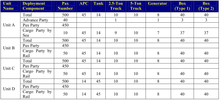
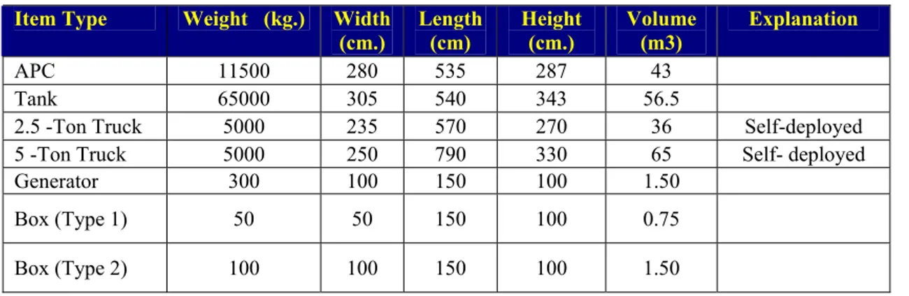
and D are co-located, and Units B and C deploy to the same destination location. The data related to the deploy-ment of each unit and its components are listed in Table 1. As shown in the line allocated to Unit A in Table 1, Unit A deploys in three components; advance, pax and cargo par-ties. The advance party for Unit A has 40 pax, one 2.5-ton truck, one generator, three Type 1 boxes, and three Type 2 boxes. The pax party for Unit A has 450 personnel. The cargo party for Unit A will deploy by sea. It has 10 pax, 45 armored personnel carriers (APCs), 14 tanks, nine 2.5-ton trucks, ten 5-2.5-ton trucks, seven generators, 37 Type 1 boxes, and 37 Type 2 boxes. Unless otherwise indicated in Table 1, each component deploys by land. The total num-ber of deployed personnel and equipment for Unit A are shown in the line named total. Units B, C, and D deploy in two components each. Their cargo parties deploy by rail as indicated in Table 1. Table 2 lists the dimensions, weight and volume information of deployed equipment used in our simulation. For example, the first line in Table 2 indicates that an APC used in this deployment weighs 11500kg.s (11.5 tons), has a volume of 43 m3. Its width, length, and height are 280, 535, and 287 centimeters, re-spectively. The minimum and maximum time require-ments for deployed units to be at their designated destina-tion locadestina-tions (not shown) and the initial delay times for each deployment component, that are used to ensure timely and coordinated arrivals at destinations for each deploying unit (not shown), are also taken into ac-Table 1: Units and Their Equipment
Unit
Name Deployment Component Number Pax APC Tank 2.5-Ton Truck Truck 5-Ton Generator (Type 1) Box (Type 2) Box
Total 500 45 14 10 10 8 40 40 Advance Party 40 1 1 3 3 Pax Party 450 Unit A Cargo Party by Sea 10 45 14 9 10 7 37 37 Total 500 45 14 10 10 8 40 40 Pax Party 450
Unit B Cargo Party by
Rail 50 45 14 10 10 8 40 40 Total 500 45 14 10 10 8 40 40 Pax Party 450 Unit C Cargo Party by Rail 50 45 14 10 10 8 40 40 Total 500 14 45 10 10 8 40 40 Pax Party 450 Unit D Cargo Party by Rail 50 14 45 10 10 8 40 40
Table 2: Dimensions and Weights of Deployed Equipment
count in the simulation model. The simulation for this scenario is a terminating one with a termination time of 240 hours. The transportation assets allocated to this sce-nario are not listed in detail here. They include one large RoRo ship, four trains with enough and appropriate rail cars, trucks, and tank carriers (one tank carrier can carry a single tank or 2 APCs). The armored vehicles must be car-ried by rail or sea to distances over 300 km. In this sce-nario, they deploy over 300 km. Other restrictions used in the simulation, such as the storage capacities of SPOE, SPOD, RPOE, and RPOD, are not presented here. Our performance measure is the percentage of on-time arrivals (averaged across replications) for each unit to their desig-nated destinations.
4.2 Design of Experiments
DOE deals with different fields from medicine to farming, and provides procedures for efficient conduct of statistical experiments. Computer simulation provides a vast area in which to expand DOE. Some of the possible designs are presented in the Design Toolkit (Kleijnen et al. 2005). Lat-in Hypercube (LH) designs are recommended for simula-tion experiments with minimal assumpsimula-tions and many fac-tors. Ye developed an algorithm for orthogonal LH designs (Ye 1998). This was later extended by Cioppa and Lucas, who gave up small amounts of orthogonality for better space-filling designs, and developed the Nearly Or-thogonal Latin Hypercube (NOLH) designs (Cioppa and Lucas 2007). Orthogonal Latin Hypercube (OLH) and NOLH designs are special cases of LH designs. OLH de-signs have strict orthogonal properties, i.e., a matrix condi-tion number of 1, and a maximum pairwise correlacondi-tion of zero between any two columns in the design matrix. NOLH designs relax the requirements on the orthogonal properties. NOLH designs choose the most space-filling design among design matrices that satisfy near orthogonal thresholds. In a good space-filling design, the design
points are required to be scattered throughout the experi-mental region with minimal unsampled regions. The limits used by Cioppa and Lucas are a condition number of less than 1.13 and a maximum pairwise correlation between all columns of the design matrix in the interval (-.03, .03) (Cioppa and Lucas 2007). The NOLH design matrix is a compromise between complete enumerations of all possi-ble scenarios, which is an exhaustive task even with to-day’s computing power, and an OLH design. NOLH de-signs can also handle discrete variables, as opposed to LH designs which can only handle continuous variables, at a cost of orthogonality and space-filling properties if the lev-els of discrete variables are a few. Generating these de-signs is a time-consuming process. But a catalogue of ready-to-use designs are available online. This paper util-izes a 29-factor and 257-run design by (Sanchez and Her-nandez 2005). Table 3 provides the factors and their levels for experimentation with our deployment simulation. The levels of these factors are entered into the spreadsheet pro-vided by Sanchez and Hernandez to create a nearly-orthogonal and space-filling 257-run design matrix. The factors are the convoy speed, the number of load and un-load docks at transfer points (such as SPOE/RPOE etc.) and minor/medium/major breakdown probabilities for transportation assets used in the deployment. These factors were chosen according to expert opinion. As more units are added, more factors with varying levels will have to be considered.
5 RESULTS
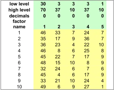
Part of the design matrix (first 10 runs for the first 5 fac-tors) created using the factors and their levels in Table 3 are presented in Table 4. For each of these input combina-tions (rows) of our 257-run design matrix (partly depicted in Table 4), we have written a script to modify the simula-tion’s base-case XML scenario file. We made 15 replica-tions (to achieve the desired accuracy of 90% relative pre-Item Type Weight (kg.) Width
(cm.) Length (cm) Height (cm.) Volume (m3) Explanation
APC 11500 280 535 287 43
Tank 65000 305 540 343 56.5
2.5 -Ton Truck 5000 235 570 270 36 Self-deployed
5 -Ton Truck 5000 250 790 330 65 Self- deployed
Generator 300 100 150 100 1.50
Box (Type 1) 50 50 150 100 0.75
cision) of each of the newly-created 257 scenarios to reach a total of 257x15=3855 computer runs. Compare this to an experiment with 29 factors each with only 2 levels and 15 replications per run for a complete enumeration experiment (229 x15= 8,053,063,680 computer runs!). We have written a VBA script to extract and calculate the percentage of on-time arrivals for each run (averaged across replications) from the simulation output files written onto EXCEL spreadsheets. For Unit A, Averaged on-time Arrivals at its destination (AoA) ranged between 76.8% and 100% with a average of 97.93% and a standard deviation of 0.0374. That is, on average, 97.93 percent of all vehicles of Unit A arrived at their destination on-time according to the de-ployment plan. For Units B and C deploying to the same destination, AoA ranged between 96% and 100% with an average of 99.96% and a standard deviation of 0.0034. The deployment plans for Units B and C seem to be robust across the input combinations simulated. For Unit D, AoA ranged between 93.04% and 98.8% with an average of 98.57% and a standard deviation of 0.0118.
Table 3: Factors and Their Levels
# Factor Name Low High
1 Convoy speed 30 70
2 Unit A Sea Group # load docks 3 37 3 Unit A Destination # unload docks 3 10 4 Unit B Home # load docks 3 37 5 Unit B RPOE # load docks 1 10 6 Unit B RPOD # unload docks 1 6 7 Unit B Destination # unload docks 3 37 8 Unit C Home # load docks 3 20 9 Unit C RPOE # load docks 1 10 10 Unit D Home # load docks 3 37 11 Unit D RPOE # load docks 1 6 12 Unit D RPOD # unload docks 1 6 13 Unit D Destination # unload docks 3 37 14 Truck Minor Breakdown Probability 0 0.05 15 Truck Medium Breakdown Prob. 0 0.07 16 Ship Minor Breakdown Probability 0 0.1 17 Ship Medium Breakdown Prob. 0 0.008 18 Train Minor Breakdown Probability 0 0.06 19 Train Medium Breakdown Prob. 0 0.02 20 Train Major Breakdown Probability 0 0.001 21 Bus Minor Breakdown Probability 0 0.05 22 Bus Medium Breakdown Probability 0 0.025 23 Bus Major Breakdown Probability 0 0.008 24 Tank Minor Breakdown Probability 0 0.1 25 Tank Medium Breakdown Prob. 0 0.04 26 Tank Major Breakdown Probability 0 0.008 27 APC Minor Breakdown Probability 0 0.15 28 APC Medium Breakdown Prob. 0 0.025 29 APC Major Breakdown Probability 0 0.009
To identify which factors contribute more to our per-formance measure of AoA, we use a nonparametric ap-proach, namely regression trees, to reveal the structure in the data in a more human-readable way. We append the AoA response variable for Units as 30th column to the 257-run design matrix for 29 factors, and import this newly formed 30-column matrix into JPM (SAS 2005).
Table 4: 10 Runs for First 5 Factors of 257-Run Matrix
low level 30 3 3 3 1 high level 70 37 10 37 10 decimals 0 0 0 0 0 factor name 1 2 3 4 5 1 46 33 7 24 7 2 35 17 9 36 7 3 36 23 4 22 10 4 46 8 6 25 8 5 45 22 7 17 9 6 48 15 10 8 9 7 32 24 6 7 6 8 45 4 6 17 9 9 33 21 10 24 4 10 49 6 9 27 1
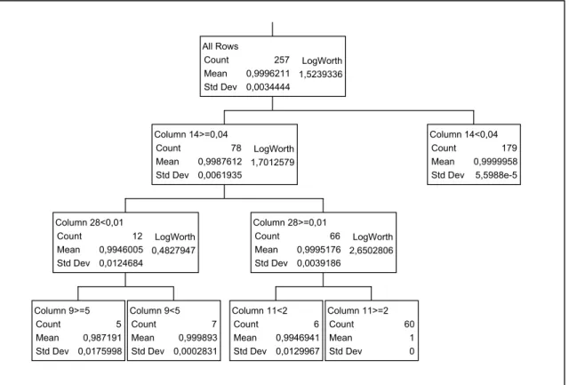
This is done separately for Unit A, Unit D, and Units B&C. The data are split into two leaves in such a way that the va-riability in the response within each leaf decreases and the variability in the response between leaves increases (Kang, Doerr, and Sanchez 2006). The split is continued until the point of diminishing returns in the value of R2 (a measure of the amount of variance in the data that is explained by the given model) is reached. Only after 26 splits, an R2 of 0.617 is reached for Unit A. For Units B and C, an R2 val-ue of 0.317 is reached only after JMP makes 6 splits, and no further splits can be made. However, a careful exami-nation of the split columns (factors) reveal that two factors have nothing to do with the deployment of Units B and C , and thus can be pruned to achieve an almost the same level of R2 of 0.314. Figure 1 shows the final regression tree for Units B and C. For (column) factor 11 (the number of load docks at RPOE for Unit D), the AoA is 100% for 60 sce-narios when number of load docks is greater than 2, as op-posed to an AoA of 99.4% for 6 scenarios when the num-ber of load docks is less than 2. Although not a huge difference, this is due to the fact that Units C and D are co-located and share the same resources (loading docks) even though the design matrix is for deployment of Units B and C. Major factors of influence seem to be minor breakdown of trucks and medium breakdown of Armored Personnel Carriers (APCs). As for Unit D, JMP makes 43 splits of the data to achieve an R2 of 0.417. A careful examination of splits and pruning of unnecessary and illogical leaves (i.e.
reveals that the same R2 value can be achieved with only 11 splits of the data.
Regression metamodels (though harder to interpret) may help validate the regression tree results to determine which factors have the greatest influence on the response variable of interest. We also fit regression models. With 29 input variables, generating a model including interac-tions for a given performance measure can be tedious. Thus, we used mixed stepwise regression, where JMP software package alternates forward and backward step-wise regression until the remaining terms are significant, to select a subset of the input variables. In the backwards se-lection, terms are brought into the model and then the least significant terms are removed until all the remaining terms are significant. It is the opposite in the forward selection
case where the most significant term is brought into the model. After stepwise regression is used to determine a model of interest, the model is fit to a linear regression us-ing standard least squares. Once fit, three statistics, ad-justed R2, the F test statistic, and the Student’s t-test statis-tic, are examined to decide on the goodness and applicability of the model. In our case, linear models did not suffice and we had to fit nonlinear models with interac-tion terms (details not included due to page limitainterac-tions). Other explanatory tools such as interaction profiles are not included in this paper for the same reason.
Figure 1: Regression Tree for Units B and C
All Rows Count Mean Std Dev 257 0,9996211 0,0034444 1,5239336 LogWorth Column 14>=0,04 Count Mean Std Dev 78 0,9987612 0,0061935 1,7012579 LogWorth Column 28<0,01 Count Mean Std Dev 12 0,9946005 0,0124684 0,4827947 LogWorth Column 9>=5 Count Mean Std Dev 5 0,987191 0,0175998 Column 9<5 Count Mean Std Dev 7 0,999893 0,0002831 Column 28>=0,01 Count Mean Std Dev 66 0,9995176 0,0039186 2,6502806 LogWorth Column 11<2 Count Mean Std Dev 6 0,9946941 0,0129967 Column 11>=2 Count Mean Std Dev 60 1 0 Column 14<0,04 Count Mean Std Dev 179 0,9999958 5,5988e-5
6 FINAL REMARKS
We have briefly described our simulation model for mili-tary deployment and showed the application of an intelli-gent design of experiments approach in the analysis of a typical deployment scenario. Not all the explanatory tools available in the further analysis of the deployment scenario could be elaborated upon here. Yet, we have presented the general approach of analysis using a NOLH design. ACKNOWLEDGMENTS
The authors would like to thank Mr. Erhan Çınar and Mr. Murat Durmaz of BilgiGIS Ltd. of Ankara, Turkey for sharing their expertise in GIS, providing guidance and help in integrating their GIS software, GeoKIT, with our simu-lation model. In addition, we thank Prof. Thomas Lucas and COL. Andy Hernandez of NPS for their insights and help on NOLH designs.
REFERENCES
Akgün, İ. and Tansel, B. 2007. Optimization of Transpor-tation Requirements in the Deployment of Military Units. Computers and Operations Research, Volume 34(4): 1158 – 1176.
Buss, A. 2001. Basic Event Graph Modeling. Simulation News Europe, 31: 1-6.
Buss, A. and Sanchez, P. J. 2002. Building Complex Mod-els With LEGOS (Listener Event Graph Objects). Proceedings of the 2002 Winter Simulation Confer-ence, ed., E. Yücesan, C-H. Chen, J. L. Snowdon, and J. M. Charnes, 732-737. Institute of Electrical and Electronics Engineers, Piscataway, New Jersey. Cioppa, T. M., and Lucas, T. W. 2007. Efficient Nearly
Orthogonal and Space Filling Latin Hypercubes. Technometrics 49(1):.
Kang, K., Doerr, K. H., and Sanchez, S. M. 2006. A De-sign of Experiments Approach to Readiness Risk Analysis. Proceedings of the 2006 Winter Simulation Conference, ed., L. F. Perrone, F. P. Wieland, J. Liu, B. G. Lawson, D. M. Nicol, and R. M. Fujimoto, 1332-1339.Institute of Electrical and Electronics En-gineers, Piscataway, New Jersey.
Kleijnen, J. P. C., Sanchez, S. M., Lucas, T. W., and Ciop-pa, T. M. 2005. A User’s Guide to the Brave New World of Simulation Experiments. INFORMS Journal on Computing, 17(3): 263-289.
Sanchez, S. M. and Hernandez, A. S. 2005. NOLHdesigns Spreadsheet. Available online via
<http://diana.cs.nps.navy.mil/SeedLa b/> [accessed 12/19/2007].
SAS. 2005. JMP User’s Guide, Version 6: SAS Institute Inc. Cary, NC, USA.
Sargent, R. G. 1988. Event Graph Modeling for Simulation with an Application to Flexible Manufacturing Sys-tems. Management Science 34(10) : 1231-1251. Sargent, R. G. 2001. Some Approaches and Paradigms for
Verifying and Validating Simulation Models. Pro-ceedings of the 2001 Winter Simulation Conference, ed., B. A. Peters, J.S. Smith, D. J. Mederios, and M. W. Rohrer, 106-114. Institute of Electrical and Elec-tronics Engineers, Piscataway, New Jersey.
Schruben, L. 1983. Simulation Modeling with Event Graphs. Communications of the ACM 26(11): 957-963.
Ye, K.Q. 1998. Orthogonal Column Latin Hypercubes and Their Applications in Computer Experiments. Journal of the American Statistical Association, 93: 1430-1439.
Yıldırım, U. Z, Sabuncuoğlu, İ., and Tansel, B. 2007. A Simulation Model for Military Deployment. Proceed-ings of the 2007 Winter Simulation Conference, eds., S.G. Henderson, B. Biller, M.-H. Hsieh, J. Shortle, J.D. Tew, and R.R. Barton, 1361-1369. Institute of Electrical and Electronics Engineers, Piscataway, New Jersey.
AUTHOR BIOGRAPHIES
UĞUR ZİYA YILDIRIM is a Major in the Turkish Ar-my. He received his B.S. and M.S. in Operations Research from the U.S. Military Academy in 1991 and from the Na-val Postgraduate School in 1999 respectively. He is cur-rently a Ph.D. candidate at the Department of Industrial Engineering at Bilkent University in Ankara, Turkey. His e-mail address is <[email protected]>.
İHSAN SABUNCUOĞLU received his Ph.D. degree in Industrial Engineering from the Wichita State University. Prof. Sabuncuoğlu teaches and conducts research in the ar-eas of simulation, scheduling, AI, and manufacturing sys-tems. He has been a visiting professor at the Wichita State. He has published papers in IIE Transactions, Decision Sci-ences, International Journal of Production Research, Simulation, Journal of Manufacturing Systems, tional Journal of Flexible Manufacturing Systems, Interna-tional Journal of Computer Integrated Manufacturing, Computers and Operations Research, European Journal of Operational Research, Journal of Operational Research Society, Computers and Industrial Engineering, Interna-tional Journal of Production Economics, Journal of Intel-ligent Manufacturing, OMEGA-International Journal of Management Sciences, and Production Planning and Con-trol. Honors Societies; Alpha Pi Mu (National Industrial Engineering Honor Society). Prof. Sabuncuoğlu is the chairman of the Industrial Engineering Department. His e-mail address is <[email protected]>.
BARBAROS TANSEL received his Ph.D. degree in In-dustrial and Systems Engineering from the University of Florida, Gainesville (U.S.A.) in 1979. Prior to his ap-pointment at Bilkent, he has served as a faculty member at the Middle East Technical University, Georgia Institute of Technology, and the University of Southern California. He has been a faculty member of the Department of Industrial Engineering at Bilkent University since 1991. His primary research interests are in network location theory, location and layout optimization, theory of optimization with im-precise data, hub location modeling and optimization, and logistics system design. Prof. Tansel’s research articles have been published in Management Science, Operations Research, Transportation Science, IIE Transactions, Jour-nal of the OperatioJour-nal Research Society, European JourJour-nal of Operational Research, International Journal of Produc-tion Research, and Journal of Manufacturing Systems. His e-mail address is <[email protected]>.
AHMET BALCIOĞLU is a Major in the Turkish Army. He received his B.S. in Business Administration from the Turkish Military Academy in 1993 and his M.S. in Opera-tions Research from the Naval Postgraduate School in 2000. His e-mail address is <[email protected]>.