WIND ASSESSMENT FOR SITES IN LIBYA AND PREDICT OF ANNUAL ENERGY

WIND ASSESSMENT FOR SITES IN LIBYA AND

PREDICT OF ANNUAL ENERGY

Fauzi Ammar SHTEWI

2021

MASTER THESIS

ENERGY SYSTEMS ENGINEERING

Thesis Advisor

WIND ASSESSMENT FOR SITES IN LIBYA AND PREDICT OF ANNUAL ENERGY

Fauzi Amar SHTEWI

T.C.

Karabük University Institute of Graduate Programs Department of Energy Systems Engineering

Prepared as Master Thesis

Thesis Advisor

Prof. Dr. Mehmet ÖZKAYMAK

Karabük March 2021

I confirm that this Master thesis entitled "WIND ASSESSMENT FOR SITES IN LIBYA AND PREDICT OF ANNUAL ENERGY" prepared by Fauzi SHTEWI is suitable as a Master thesis.

Prof. Dr. Mehmet ÖZKAYMAK ... Thesis Advisor, Department of Energy Systems Engineering

KABUL

This thesis is accepted by the examining committee with a unanimous vote in the Department of Energy Systems Engineering as a Master thesis. March ,2021

Examining Committee Members (Institutions) Signature

Chairman : Prof. Dr. Mustafa AKTAŞ (GÜ) ...

Member : Prof. Dr. Mehmet ÖZKAYMAK (KBÜ) ...

Member : Doç. Dr. Engin GEDİK (KBÜ) ...

The degree of Master of Science by the thesis submitted is approved by the Administrative Board of the Institute of Graduate Programs, Karabük University.

“I declare that all the information within this thesis has been gathered and presented in accordance with academic regulations and ethical principles and I have according to the requirements of these regulations and principles cited all those which do not originate in this work as well.”

ABSTRACT

M. Sc. Thesis

WIND ASSESSMENT FOR SITES IN LIBYA AND PREDICT OF ANNUAL ENERGY

Fauzi Ammar SHTEWI

Karabük University Institute of Graduate Programs Department of Energy Systems Engineering

Thesis Advisor:

Prof. Dr. Mehmet ÖZKAYMAK March 2021, 61 pages

For sites in Libyan were selected for technical and economical assessment of wind power generation using real measured wind data. The assessment was carried out using the Weibull distribution function and the Weibull parameters were calculated using three different methods; For example, graphical method (GM), empirical method (EM) and so on. Error analyses using various techniques were conducted to check for the validity of the different Weibull methods used. The technical assessment includes the calculations of the annual energy production (AEP), capacity factor (Cf). The estimated annual energy production was used in the calculation of the present value of cost which estimates the cost of each kWh of electricity produced by a certain wind turbine. Adding the GHG reduction income into the electricity cost calculations decreases it by an average of (16% - 19%).

ÖZET

Yüksek Lisans Tezi

LİBYA'DAKİ SAHALAR İÇİN RÜZGÂR DEĞERLENDİRMESİ VE YILLIK ENERJİ TAHMİNİ

Fauzi Ammar SHTEWI

Karabük Üniversitesi Lisansüstü Eğitim Enstitüsü

Enerji Sistemleri Mühendisliği Anabilim Dalı Tez Danışmanı:

Prof. Dr. Mehmet ÖZKAYMAK Mart 2021, 61 sayfa

Gerçek rüzgâr verileri kullanılarak Libya daki sahalar için rüzgâr enerjisi üretiminin teknik ve ekonomik değerlendirmesi yapıldı. Weibull dağılım işlevi kullanılarak teknik değerlendirme, yıllık enerji üretimi (AEP), kapasite faktörü (Cf) hesaplamaları yapıldı ve Weibull parametreleri üç farklı yöntem kullanılarak hesaplandı; Örneğin, grafiksel yöntem (GM), ampirik yöntem (EM) vb. Kullanılan farklı Weibull yöntemlerinin geçerliliğini kontrol etmek için çeşitli teknikler kullanılarak hata analizleri yapılmıştır. Teknik değerlendirme, yıllık enerji üretimi (AEP), kapasite faktörü (Cf) hesaplamalarını içerir. Tahmini yıllık enerji üretimi, belirli bir rüzgâr türbini tarafından üretilen her bir kWh elektriğin maliyetini tahmin eden mevcut maliyet değerinin hesaplanmasında kullanılmıştır. Sera gazı azaltma gelirini elektrik maliyeti hesaplamalarına eklemek, onu ortalama (% 16 -% 19) oranında düşürür.

ACKNOWLEDGMENT

This report provides an explanation and it is written to provide background material and beneficial information for students. We hope students and readers benefit from our report and understand it.

I would like to express my sincere thanks to my advisor, Prof. Dr. Mehmet Özkaymak for their valuable comments and suggestions in the progress of this study. I would like to thank all of my friends who helped me in continue this research and also thanks to all of my family.

CONTENTS Page APPROVAL ... ii ABSTRACT ... iv ÖZET... v ACKNOWLEDGMENT ... vi CONTENTS ... vii LIST OF FIGURES ... x

LIST OF TABLES ... xii

SYMBOLS AND ABBREVIATIONS INDEX... xiii

PART 1 ... 1

INTRODUCTION ... 1

1.1. CAUSES OF THE WIND POWER ... 1

1.2. WIND ENERGY APPLICATIONS ... 3

1.3. TYPES OF WIND TURBINES ... 3

1.4. WIND SPEED MEASUREMENTS ... 4

1.4.1. Instruments ... 5

PART 2 ... 7

ENERGY AND LITERATURE REVIEW ... 7

2.1. ENERGY OF LIBYA ... 7

2.1.1. The Current Oil Situation ... 7

2.1.2. The Natural Gas Current Situation ... 9

2.1.3. The Current Electricity Situation ... 10

2.1.4. Load Growth in Libya ... 12

2.1.5. Renewable Energy in Libya... 14

2.1.5.1. Solar Energy... 14

Page

PART 3 ... 21

METHODOLOGY OF WIND ASSESSMENT ... 21

3.1. SITING OF MONITORING SYSTEMS ... 21

3.1.1. Preliminary Area Identification ... 22

3.1.2. Area Wind Resource Evaluation ... 22

3.2. MEASUREMENT PLAN ... 22

3.3. MONITORING DURATION AND DATA RECOVERY ... 23

3.4. USE OF WIND DATA SOURCE ... 23

3.5. CHARACTERISTICS OF THE WIND ... 24

3.6. WIND DATA COLLECTION ... 25

3.7. WIND DATA ANALYSIS ... 25

3.7.1. Wind Speed Variation with Height... 25

3.7.2. Functions Distribution ... 26

3.7.2.1. Rayleigh Distribution ... 27

3.7.2.2. Weibull Distribution ... 27

3.8. ERROR ANALYSIS ... 29

3.9. MEAN WIND SPEED ... 30

3.10. WIND POWER DENSITY ... 30

3.11. OPERATIONAL CHARACTERISTICS... 30

3.11.1. Power Performance ... 30

3.11.2. Annual Energy Production ... 31

3.11.3. Availability ... 32

3.12. PRESENT VALUE COST AND ELECTRICITY PRICE ... 33

PART 4 ... 35

RESULT ... 35

4.1. WIND DATA ... 35

4.2. WEIBULL PARAMETERS... 40

4.3. PROBABILITY DENSITY AND CUMULATIVE DISTRIBUTION FUNCTION ... 43

Page 4.5. ANNUAL ENERGY PRODUCTION AND CAPACITY FACTOR

RESULTS ... 49

4.6. PRESENT VALUE COST AND ELECTRICITY PRICE RESULTS ... 51

4.7. GREENHOUSE GASES EMISSION REDUCTION ... 53

PART 5 ... 55

CONCLUSION ... 55

REFERENCES ... 57

LIST OF FIGURES

Page

Figure 1.1. Win circulation. ... 2

Figure 1.2. Global wind flows... 2

Figure 1.3. Horizontal &vertical axis wind turbines. ... 4

Figure 1.4. Cup anemometer. ... 5

Figure 1.5. Propeller anemometers in fixed three-dimensional arrangement. ... 5

Figure 1.6. Ultrasonic anemometer. ... 6

Figure 1.7. Remote sensing. ... 6

Figure 2.1. Libya crude oil production from 2010 to 2015 ... 8

Figure 2.2. The distribution of the oil resource in Libya. ... 9

Figure 2.3. The natural gas production and consumption from 2000 to 2013 ... 9

Figure 2.4. Locations of the electrical power plants ... 10

Figure 2.5. Types and percentage of gas and fuel used in electricity 2012. ... 11

Figure 2.6. Types and shares of customers of Libyan electricity in 2012. ... 11

Figure 2.7. The 400 kV Libyan transmission systems. ... 12

Figure 2.8. The energy consumption over the last 10 years. ... 13

Figure 2.9. Expected load demand for the next 20 years. ... 13

Figure 2.10. The monthly solar radiation in different cities in Libya. ... 15

Figure 2.11. The load profile and the average temperature throughout the year. ... 16

Figure 2.12. The monthly average wind speed in different cities in Libya. ... 16

Figure 2.13. The Libyan renewable energy plan... 18

Figure 3.1. Power output from wind turbine as function of wind speed. ... 31

Figure 4.1. Location of sites. ... 36

Figure 4.2. Monthly variation of wind speeds for the selected sites (20m). ... 38

Figure 4.3. Monthly variation of wind speeds for the selected sites (60m). ... 38

Figure 4.4. Annual mean wind speeds for the selected sites at 20m height. ... 39

Page

Figure 4.6. Measured annual frequency distribution (20m). ... 40

Figure 4.7. Measured annual frequency distribution (60m). ... 40

Figure 4.8. Graphical method to estimate the Weibull parameters at 20m. ... 41

Figure 4.9. Graphical method to estimate the Weibull parameters at 60m. ... 42

Figure 4.10. Comparison of the probability density function 20m. ... 44

Figure 4.11. Comparison of the probability density function 60m. ... 45

Figure 4.12. Cumulative distribution function for the sites at 20m height. ... 46

Figure 4.13. Cumulative distribution function for the sites at 60m height. ... 47

Figure 4.14. Power curve of the model wind turbine. ... 50

Figure 4.15. Comparison of AEP among sites using different Weibull methods 60m. ... 51

LIST OF TABLES

Page

Table 3.1.Wind speed parameters for calculating a vertical profile ………26

Table 4.1. Physical features of the meteorological stations. ... 36

Table 4.2. Average wind speeds (20m). ... 37

Table 4.3. Average wind speeds (60m). ... 37

Table 4.4. Weibull Parameters estimated by three different 20m. ... 43

Table 4.5. Weibull Parameters estimated by three different 60m. ... 43

Table 4.6. Error analysis results (20m). ... 48

Table 4.7. Error analysis results (60m). ... 48

Table 4.8. Technical specifications of the model wind turbine. ... 49

Table 4.9. Annual energy production and capacity factor for all sites (60m). …….51

Table 4.10. The values of the terms in the present value cost equation………..52

Table 4.11. Electricity cost of each kWh for each site 60m. ... 52

Table 4.12. Annual GHG reduction for each site 60m ... 53

SYMBOLS AND ABBREVIATIONS INDEX SYMBOLS bbl : barrel GW : Gigawatt MM : Millimeter PV : solar cells

R2 : square of the ratio

ABBREVIATION

AEP : Annual Energy Production

CDF : Cumulative Distribution Function CF : Capacity Factor

D : Day

EM : Empirical Method

GECOL : General Electricity Company of Libya GM : Graphical Method

GHG : Green House Gases KV : Kilo Volt

KWh : Kilo watt hour

MLM : Maximum Likelihood Method MBE : Mean Bias Error

MAE : Mean Absolute Error MW : Mega watt

M : Meter

PDF : Probability Density Function PVC : Present Value Cost

RMSE : Root Means Square Error

REAOL : Renewable Energy Authority Of Libya S : Second

PART 1

INTRODUCTION

For thousands of years, wind has been utilized as a source of energy. During the seventeenth and eighteenth centuries, it was one of the most used sources of energy for mankind, along with hydro power. The first experiments on the use of windmills for electricity generation were carried out at the end of the nineteenth century. Then, there was a long period of a low interest in the use of wind power. In 1972, the international oil crisis initiated a resumption of the use of renewable resources.

1.1. CAUSES OF THE WIND POWER

The World emits the heat from the Sun constantly, but unevenly, into the atmosphere. In environments where less heat is emitted (cool air zones), where more heat is released, the air warms up and gas pressure is reduced, the temperatures on the atmospheric gases rise. As a result of convective movements, a macro-circulation is developed: air volumes are heated, densified and increase, thus drawing cooler air moving through the earth's surface. This circulation of cold and warm air masses produces high-pressure and low-pression zones that are constantly present in the atmosphere and affected by earth rotation (Figure 1.1).

Figure 1.1. Win circulation.

The air flows from places with a higher pressure to places where the pressure is lower and so the air carries a larger or lesser amount of air between zones at a different pressure, because of the atmosphere's propensity to continuously adjust the pressure balance. As the atmosphere attempts to restore the equilibrium of pressure constantly, the air travels from areas where the pressure is greater than that where it is smaller. Therefore, the wind is more or less easy to transfer the air mass between zones. The wind does not necessarily blow in the direction that joins the core of the higher pressure and the northern portion but, in the north, it turns to the right and rotates in the clockwise direction around the high-pressure centers and in the low-pressure centers. The bigger the gaps in pressure, the quicker the air flow and hence the stronger the breeze, the person who is heading back to the wind has 'B' on his left and 'A' on his right side (Figure 1.2). In the southern hemisphere the reverse is happening.

At different latitudes the circulation of air masses that is cyclically influenced by each season can be observed on a large scale. Separate heating is achieved on a smaller scale between dry land and water masses, resulting in regular sea and ground breezes. The winds and their local characteristics are influenced greatly by the profile and uniformity of the dry land or surface of the water, and indeed the wind blows with additional intensity on wide and smooth surfaces such as the sea. This is the central issue for wind turbines. Outside the sea. Furthermore, on top of the rises or in the valleys, aligned in parallel to the present wind direction, the wind is stronger, while on uneven areas, such as the towns or forests, it slows down, and the atmospheric equilibrium in terms of the height above the earth determines its speed [1].

1.2. WIND ENERGY APPLICATIONS

Wind turbines can be used as separate devices, or they may either be attached to a utility power grid or may also be paired with a solar panel system. Usually, several wind turbines are built in close proximity to build a wind turbine for energy sources. Today, many electricity producers are using wind turbines to provide power to consumers. Stand-alone wind turbines are normally used for water pumping or connectivity. However, in windy regions, wind turbines can also be used to cut back on electricity prices for households, producers and farmers. Tiny wind systems also have potential as distributed energy options. The distributed energy resources are a collection of small modular technology that can be integrated with the energy delivery grid to boost its operation.

1.3. TYPES OF WIND TURBINES

There are two major types of wind turbines according to the orientation of the axis. The most popular form of large-scale wind generator is the horizontal axis, which includes the blade axis parallel to the field. For generators of the vertical axis with a blade axis perpendicular to the ground, the wind direction controls are unnecessary [2].

Figure 1.3. Horizontal &vertical axis wind turbines.

1.4. WIND SPEED MEASUREMENTS

The measured wind atmosphere is the primary input for the flow models, from which the spot calculation is extrapolated horizontally and vertically to assess the energy source around the site. This resource map is the basis for an optimal layout.

If the ability of flux models to accurately forecast the spatial variance of the wind reduces, the number and the height of observable stems should be modified to the complexity of the area. In order to guarantee a fair forecast of the wind resource, the more complicated the location, the more and higher masts need to be mounted. Sadly, wind measurements are often overlooked. The measuring height is most commonly insufficient for the size of the site, the number of masters insufficient for the site scale, too little time for the calculation, instrument not calibrated and installation is inadequate or the mast is not held. The costliest aspect to quantify wind is the lack of data cannot be stressed enough. Any estimation of wind resources requires a minimum measuring time of one complete year to reduce seasonal bias. If instrumentation fails due to lightning strike, glazing, vandalism, or other factors, and the fault cannot be readily detected, the findings will be falsified by the missing data. Another means of undermining the feasibility of the whole project may be the increased vulnerability.

1.4.1. Instruments

Although the energy density is equal to the cube of the average wind velocity, the calculations of the wind speed have made the instrumentation very challenging. The methods employed must furthermore be robust and effective data collection over long unattended operation times. The most on-site wind analyses are done using the traditional cup anemometer. The behaviour, and the causes of errors are known, are fairly well understood. The below are some of the wind velocity measurement tools.

Figure 1.4. Cup anemometer.

Figure 1.6. Ultrasonic anemometer.

PART 2

ENERGY AND LITERATURE REVIEW

2.1. ENERGY OF LIBYA

As an ultimate means of energy production, Libya currently relies on gas and oil. All of these conventional properties are reduced and exhausted. With the rapid rise in energy demand in Libya, oil and natural gas production can be impacted. This leads to a drop in wages. This moved Energy Authority towards investing in renewable energy quickly and not well prepared. According to the REAOL (Libyan Clean Energy Authority), the share of renewable energy is expected to cross 10 percent in 2025 [3].

The proposed schemes mostly include solar and wind power systems. The creation of this modern technology raises various obstacles. Both proposed schemes are funded by the General Electrical Company of Libya, a government-owned company which is not able to privatise or compete. Any renewables are postponed or halted as a consequence of the inconvenient preparation. The work to be done in this direction is therefore one of the steps. To produce its energy needs, Libya depends entirely on fossil fuels. The primary sources of energy are oil and natural gas. The energy plants in Libya, with rising reliance on natural gas, have relied in recent years on light and heavy oil. The next was a review of Libya's energy.

2.1.1. The Current Oil Situation

Libya is one of the largest oil producers in North Africa and reportedly accounts for about one million barrels per day, compared to 1.68 million bbl/d in February 2011, previous to the civil war. About 47.1 billion barrels of the existing proven oil reserves are[4].

Figure 2.1 presents the output of crude oil over the last five years. In February 2011, oil production stopped due to incidents [2]. The country's situation improved during 2012 and 2013, with production settling at about 1.4 million bbl / d. Oil production was halted in mid-2013 due to the spread of the militias that took control of several major refineries and oil harbors.

Figure 2.1. Libya crude oil production from 2010 to 2015 [2].

Before the 2011 incidents, National Oil Corporation (NOC) was the main petroleum industry participant. This target will not be met until production volumes come back into their levels before the 2011 war, but the 2015 NOC is set at 2.5 million bbl/d. This recovery requires a stable environment and rest to enable foreign companies to begin oil exploration in Libya. Most oil in Libya is found in the Eastern part of the country (as shown by Figure 2.2, this region is called the Sirte Basin) and about 25 per cent in the South (this is the Murzuk Basin). Total oil production in Libya is about 1.8 million bbl/d and about 300.000 bbl/d for power generation. This number would be raised by the rise in energy consumption.

Figure 2.2. The distribution of the oil resource in Libya [2].

2.1.2. The Present Situation of Natural Gas

The second highest production resource is Natural Gas. The proven reserves of natural gas estimated in 2012 are 52.8 trillion cubic feet. Figure 2.3 illustrates how Libya produces and uses natural gases.

Figure 2.3. The natural gas production and consumption from 2000 to 2013 [2].

Figure 3 indicates that much of the natural gas produced is exported. The big shift in gas supply begins when a gas pipeline begins production between Libya and Italy, where most Libyan gas is shipped to Italy [2]. The rise in gas consumption is caused by gas reliance for the manufacture of energy rather than gasoline.

2.1.3. The Present Situation of Electricity

In order to satisfy the burden demands, as shown in Figure 2.4[5] Libya has built 12 power stations. These plants are capable of producing 8,347 GW while 6,357 GW is usable. In 2012, in some transmission lines and suburbs, anarchy and the conflict of the country led to destruction, with the unnecessary use of air conditioners, peak demand amounted to 5,8 GW in summer. In addition, the increased number of unauthorized buildings makes it difficult for GECOL to provide electricity to nearly all the country's cities. In order to ensure the reliability of the grid, GECOL was forced to enforce load shedding plans and several blackouts have occurred in the last year.

Figure 2.4. Locations of the electrical power plants [5].

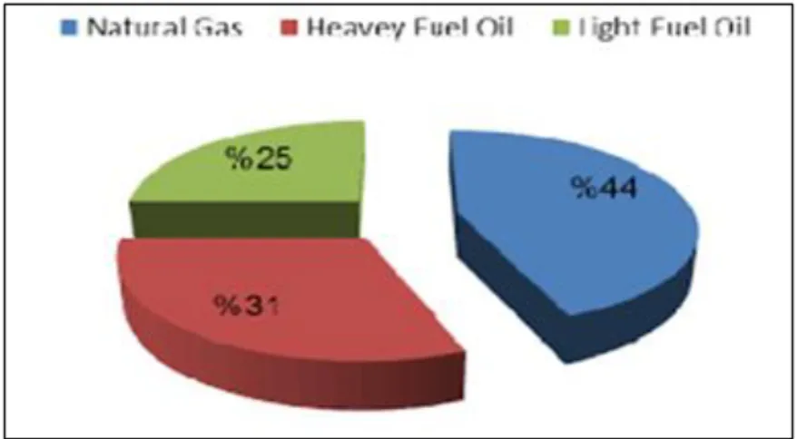
The energy market is dominated by coal, heavy fuel oil and light fuel oil, as shown in Figure 2.5. In order to reduce carbon emissions GECOL has expanded its reliance on natural gas.

Figure 2.5. Types and percentage of gas and fuel used in electricity generation in 2012.

As seen in Figure 2.6, the energy usage is spread among different charging forms. The residential fee is the dominant charge with 31 percent of the cumulative energy used.

Figure 2.6. Types and shares of customers of Libyan electricity generation in 2012.

Libya provides electricity with a total of 15 power stations via gas and steam turbines. The bulk of these stations are clustered along the coast, where the majority of the population lives, as seen in Figure 2.4 above. It should be remembered that the only sources used in generation stations to fuel turbines are gas and diesel. Energy growth will also contribute to higher oil and gas usage in the future, with higher carbon dioxide emissions and lower domestic economic incomes. Carbon dioxide emissions from electricity production are much higher in Libya than those generated by industry and

GECOL, the number of units working on fuel was decreased. The use of mixed cycle stations to limit fuel consumption was also an alternative solution. In addition, GECOL has upgraded its transmission line system to reduce network delays and improve its efficiency and reliability. The transmission grid is now about 16,000 kilometers in length (220 KV, 400 KV) while the medium voltage (33 KV, 66 KV) is about 28,000 kilometers. For many factors, such as the low local fuel prices and the non-existing energy saving regulatory framework in Libya, energy use in power, manufacturing, and transport was not rationalised in Libya. GECOL has also constructed a 400kV transmission system as an additional measure to minimise emissions of gas in response to the rising reliance on natural gas. This improves Libya's power transmission grid quality and stability. Figure 2.7 displays the proposed and built 400 kV transmission systems.

Figure 2.7. The 400 kV Libyan transmission systems.

2.1.4. Load Growth in Libya

One of the main subjects in terms of load demand prediction is the load growth analysis. The annual GECOL study showing the energy consumption of Libya over the last 10 years, as in Figure 2.8. The regression equation was derived and then used

Figure 2.8. The energy consumption over the last 10 years.

In a near future, as shown in figure 2.9 as a result of economic growth, energy consumption is projected to rise dramatically, leading to higher oil and gas use and reduced domestic economic income and higher carbon dioxide emissions. Figure 2.9 indicates the projected rise in energy demand.

Figure 2.9. Expected load demand for the next 20 years.

The demand for electricity in the long term would rise with 9 per cent, as can be predicted of Figure 2.9. This means a major rise in the volume of oil that is used for

barrel of oil can generate 1,628 kWh in three stage cycles. Second, by breaking over 1628 KWh in no barrels this oil volume can be converted. In the end, its price, estimated by OPEC, multiplies this number of barrels [6, 7].

In the 2030s, for instance, demand for loads is estimated to amount to 120 GWh, and 194 thousand barrels (bbl/d) per day to cover this generation. This amount will be decreased by about 1,3 million barrels of Libya's overall daily export. It would cost the country roughly 19,4 billion a year. This indicates that the use of electricity will lead to a significant decline in oil exports unless renewable energy technology is introduced. The use of electricity from renewables, such as wind and solar, would also limit emissions of CO2. The saving of Libya's oil and gas wealth is not only good for Libya, but for the world as a whole.

2.1.5. Renewable Energy in Libya

In 2020, 20 per cent of the power generated will be made. Projects planned are mostly solar and wind energy systems. In 2020, Libya will produce about 20% of its electricity from solar energy. This would be approximately 3 GW (20 percent of approximately 15 GW). Nevertheless, Libya’s actual share of renewable energy is negligible.

2.1.5.1. Solar Energy

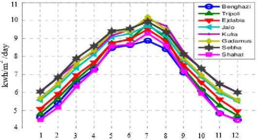
Libya is one of the countries with strong solar energy blessings because of its geographical location. It is thought that Solar Energy is the most effective and viable source of green energy in Libya. Sunny areas (between 150N and 350N) are situated within the most desirable Libyan zone. In most areas of the world the rainfall is less than 150 mm. The average solar radiation in Libya, for example, is approximately 7.5 kWh/m2/day and approximately 3000-3500 hours of sunlight a year [5]. Figure 2.10 displays solar radiation in numerous Libyan cities.

Figure 2.10. The monthly solar radiation in different cities in Libya.

As is visible from Figure 2.10 during the summer with heavy solar radiation. The maximum load increases significantly in the summer hottest months (June, July, Aug, Sept and Oct). The primary explanation is that the irrational use of air conditioners is excessive. In the coldest months of the year (Jan, Fab and Dec), load demand also increased. In order to demonstrate that effective peak load shaving can be accomplished using solar energy, the behavior of electrical loads in Libya and of sun radiation in the area has been studied. Figure 2.11 displays the load profile based on the one-year maximum load and the region's measured temperature. The connection between the temperature and the requirements of the load is evident in the figure.

Figure 2.11. The load profile and the average temperature throughout the year.

2.1.5.2. Wind Energy Resource

The second-best source of green energy is wind energy. Figure 2.12 shows wind strength in some cities of Libya, the average wind speed at three different heights ranges between (4.5 ~ 8.5 m / s).

Back to Figure. 2.10, the peak in load demand can be shaved in the summer with the penetration of solar energy as the solar energy is at its best. Wind energy plays a significant role in the generation of electricity in the winter, where there is a lack of hours of sunlight. By placing the renewable energy train on the track, the anticipated increase in load requirements can be compensated for. The cost of the kWh produced by oil is 0.176 $based on the 100 $price of the crude oil price per barrel. The average cost of the kWh produced by PV in Libya is about 0.123, $which is much cheaper than the combustion of precious crude oil. Stability, stability and political wellness are what the nation needs. Libya’s energy is subsidized and it is easier for GECOL to invest in the country's emerging green technologies. Since most of the loads are residential, 44% are counted in addition to commercial loads. Excessive heating and cooling can be minimized by solar and wind energy penetration. It should be noted that street lighting accounts for about 19 percent of the load. GECOL relies on very old and inefficient systems for street lighting. It will achieve energy consumption and reduce CO2 emissions by replacing these old-fashioned, outdated technologies with LED solar street light systems.

The Libyan proposal for renewable energy is shown in Figure 2.13 for [8]. The strategy is split into four fundamental stages. This plan has been suspended due to the deteriorating situation in Libya. Due to volatility, the 6 percent target was not reached in 2015. There is also no real will to start these projects. An illustration of bad planning. The first phase of the project was the construction of a 60 MW wind farm in the city of Dernah, which would last from 2008 to 2012. The farm includes 37 wind turbines, each rated at 1.65 MW. The project is delayed due to certain issues concerning the ownership of the land used for the wind farm.

Figure 2.13. The Libyan renewable energy plan.

2.2. LITERATURE REVIEW

Several studies have been carried out in various locations for wind energy evaluation. Bhuiyan et al. [9], have carried out a wind energy assessment in Kuakata, Bangladesh using the Wind Energy Assessment software of IUT. They have implemented both of Rayleigh and Weibull methods in the calculation of wind energy production. They have also emphasized on the effects of wind energy on the greenhouse gases reduction.

Izelu et al. [10] have conducted a wind resource assessment in Port Harcourt, Nigeria. Their assessment was based on Weibull probability distribution function. The results revealed high wind energy potential in the analyzed site.

Olaofe [11], has studied the offshore wind energy assessment in the southwest coast of Nigeria using a high resolution satellite observations. The author found that the Weibull method gave better fitting for the offshore wind speed than the Rayleigh method.

Pachauri and Chauhan [12] have explored the wind technology assessment in India. They have in details presented the challenges, wind power development and marketing the small wind turbines in India.

Gualtieri [13] has developed an integrated wind resource assessment for wind farm planning. The tool is used to calculate many parameters such as mean wind speed, power density, Weibull parameters and annual energy production. The same author has upgraded this tool in [13]. The new upgrades include (but not limited to) the calculation of the wind power density function, estimation of the wind speed extrapolation to a specific hub height and uncertainty assessment for annual energy production.

SCADA data of a wind farm located in a complex terrain in Italy. The results showed that their methods are promising for future applications. Libya is a rapidly growing consumer of energy and the demand for electricity increases by 10% -15% every year [15]. Libya is one of the highest electricity consumptions per capita in Africa. The consumption has increased from 2.60 kWh in 2000 to 4.60 kWh in 2009 [16]. The general satellite data-based wind map shows that the capacity for wind energy in Libya is high. The average wind speed is between 6-7.5 m/s at 40m height [17]. There are few studies about wind energy in Libya.

ElOsta et al. [18] have selected a small wind farm of 1.5MW to be a pilot wind project. They have investigated different sites in Tripoli. Zwara site was chosen as the site of the project. The analysis was conducted using WASP software. The average wind speed was found as 6.9m/s at 10m height with an available power of 399 W/m2. Their results were promising for the wind farm project.

El-Osta and Khalifa [19] have conducted a pre-feasibility study for a 6MW wind farm in Zwara site. They have used the RET Screen software for the economic evaluation of the project. Their results show that the project is feasible.

El-Osta et al. [20] carried out an analysis to measure wind power on the central Libyan coastal area and to estimate wind energy loans for various stages of penetration. The findings show that the entire power demand can be supplied in less than 1 per cent of the total region of Lybia. They concluded that Libya has a very strong and exciting wind capacity.

The use of green energy in Libya has been studied by Mohammed et al.[21]. They concluded that Libya is green, like wind, but needs a broader energy policy and more spending in finance and education.

Elmnefi and Bofares [22] have obtained wind speed measurements for 12 months period at Benina site in Libya. The results showed an average wind speed of about 11

studies for the wind potential in Iran [23], Italy [24], Ankara [25], Algeria [26] and India [27] have also been performed.

PART 3

METHODOLOGY OF WIND ASSESSMENT

Wind capital research software is similar to most engineering programmes. It requires planning and coordination and is constrained by budget and timetable. For selection of the best assessment tool it requires a clear collection of goals. The overall productivity of the assembled programme properties, sound location and calculating approach, trained workers, quality equipment and advanced data collection technology are all dependent on this. Therefore, several characteristics concerning the results, including: For the wind data from selected stations need to be analysed carefully:

• Place the station.

• Topography of the region.

• Exposure and height of anemometer.

• Observation form (average or instantaneous). • Record length.

From the above, the wind analysis stages go through several steps, the most important of which are:

3.1. SITING OF MONITORING SYSTEMS

A variety of methods are possible for the investigation of the wind resource in a given area. The preferred solution relies on your renewable energy goals based on past expertise in the estimation of wind resources. These methods may be categorized as certain basic evaluation scales or stages for wind resources: preliminary identification of the region, evaluation of wind resource areas, etc.

3.1.1. Preliminary Area Identification

This system scans a reasonably large region (e.g. state or public sector territory) for suitable areas of wind resources on the basis of information such as airport wind records, topography, flagged trees and other indicators. New wind measuring sites can be chosen at this point.

3.1.2. Area Wind Resource Evaluation

This phase is used for wind measuring programmes to identify wind resources in a particular region or array of wind energy fields. The most common targets of this wind measuring scale are:

• Verify or determine whether wind services are sufficient in the area to justify additional site-specific investigations.

• Compare areas to discern between relative opportunities for growth.

• Determine or verify if within the area there are enough wind resources to warrant further site-specific investigations.

• Screen for future construction locations of wind turbines.

3.2. MEASUREMENT PLAN

The requirement for a calculation plan is common to all monitoring schemes. It helps to ensure that the wind control platform covers all facets that include the information required to meet the objectives of the wind energy programme. Therefore, the aims of the initiative should inform the nature of the plan of calculation, which the project members should write down and validate and agree before its execution. The strategy should describe the following characteristics:

• Parameters of measure.

• Heights for sensor estimation.

• Minimum precision of calculation, length and data recovery. • Sample of data and intervals for recording.

• Format of data collection.

• Procedures for data collection and processing. • Measures for quality management.

• Data reporting format.

3.3. MONITORING DURATION AND DATA RECOVERY

The minimum surveillance cycle could be one year, but two years or more will provide more reliable results. One year is usually sufficient to measure the diurnal and seasonal fluctuations of the wind. With the aid of well linked, long term stations, such as an airport, the wind variability can also be measured. Data recovery for all calibrated parameters, with any data discrepancies kept to a minimum, should be at least 90% over the lifespan of the programme (less than a week). The key goal of a positioning programme is to identify potentially windy locations with other proper features of a wind energy building site. There are three phases in the sitting effort:

• Identifying wind production potential areas; • Candidate sites inspection and ranking;

• Selection of the current site(s) of the applicant tower.

3.4. USE OF WIND DATA SOURCE

Climatic data is the most common wind sources in the National Climate Data Center (which archives weather data from all National Weather Service stations), universities and air quality control.

3.5. CHARACTERISTICS OF THE WIND

The wind power available is proportional to a wind speed cube (𝑝 ∝ 𝑉_∞3 ), and thus it is important to have detailed wind information, and the output of any wind turbine is characteristic to be correctly measured. There are various wind parameters to be identified, including mean wind speed, directional data, short-term (gusts) mean variations, regular, seasonal, annual variations and height variations. These dimensions are extremely site-specific, and measurements at such sites can only be determined with reasonable precision over a period of time. The results and economics of a wind turbine are analysed. In this study we focus on collection, evaluation and analysis of existing data.

3.5.1. Variation in Time

The wind speed differences in time can be classified into the following categories:

• Inter-annual variations: This form of wind speed change happens more than one year over time. The ability to forecast a given position on an annual basis is as critical as predicting a site's long-term medium wind.

• Seasonal and monthly variation: the degree of seasonal wind variations at a given location depend on latitude and place in regard to certain topographical characteristics such as land masses and water. In winter or in spring, mountain passes in coastal areas are usually subjected to high winds and heavy winds in summer.

• Diurnal variation: Due to a deferential heating of the surface of the earth in the regular period, this form of wind speed shift is. A typical diurnal shift is the increase in wind speed during the day and the reduction in wind speed over the period between midnight and sunrise.

• Short-term shifts: Short-term variations typically reflect changes over the time span of ten minutes or less. The wind speed fluctuates and the energy content of the wind thus changes continuously. Turbulence and gusts generate

These fluctuations are in all three (longitudinal, lateral and vertical) directions when an inflammation happens in a chaotic wind field.

3.6. WIND DATA COLLECTION

For all stations measured between 2008 and 2010 wind speed data were evaluated statistically on an hourly time-series basis in this project. The wind speed data in the time range format is usually structured in a frequency distribution format because it is more useful for statistical analyses. The time series data available have been converted into frequency distribution format. At 10 m or at real height (20, 60) m, wind velocity data were collected. Both stations are constantly anemometer by a cup generator. The wind speed data collected continuously were averaged over 3 hours and stored in this project as hourly values.

3.7. WIND DATA ANALYSIS

In order to measure wind power generation at specific locations the study requires a knowledge of wind direction and wind velocity data. Long-term wind data may be used for the calculation from meteorological stations close to the candidate site. These long-term data can be extrapolated to reflect the wind profile on the future location.

3.7.1. Wind Speed Variation with Height

Wind level varies above the ground at high altitude and the wind speed changes to zero at a height of 2 km above the ground. The following studies are used to define the most typical expressions of wind speed shift with hub height [28]:

• Power law function

𝑉(𝑧) = 𝑉(𝑧_𝑟) (𝑧 𝑧_𝑟)

Where 𝑉(𝑧)the wind speed at height Z is, 𝑉(𝑧𝑟) is the reference wind speed at height

𝑍_𝑟 andα is the power law exponent which depends on the roughness of the terrain.

• Logarithmic function (log law)

𝑉(𝑧) 𝑉(10)⁄ = 𝑙𝑛(𝑍 𝑍⁄ ₀) ÷ 𝑙𝑛(10 𝑍⁄ 0) (3.2)

Where 𝑉(10) is 10 m high, the wind is 10 m high, while 𝑍₀ is roughness. Table 3.1 displays the parameters α and 𝑍0 for various field forms.

Table 3.1. Wind speed parameters for calculating a vertical profile.

Type of terrain Roughness

class Roughness length 𝒁𝟎 (m) Exponent (α) Areas of Water 0 0.001 0.01

Nation clear, few surface characteristics 1 0.12 0.12 Agriculture of hedges and houses 2 0.05 0.16 Agriculture of multiple crops, woods

and villages

3 0.3 0.28

For measuring the average wind speed at a certain height, both functions may be used, whether the mean wind speed is defined at reference height.

3.7.2. Functions Distribution

This research primarily focuses on measuring and performing cost estimates of annual energy generation at each chosen site. Information about probability density (PDF) and cumulative distribution (CDF) should be known for the estimation of annual energy supply. Typically, the PDF is given by either Rayleigh or Weibull distribution. The Rayleigh PDF and CDF are given by the mean velocity only as [28].

3.7.2.1. Rayleigh Distribution 𝑃𝐹(𝑣) =𝜋 2( 𝑣 𝑉_𝑚2) 𝑒𝑥𝑝 [− 𝜋 4( 𝑣 𝑉_𝑚) 2 ] (3.3) 𝐹(𝑣) = 1 − 𝑒𝑥𝑝 [−𝜋 4( 𝑣 𝑉𝑚) 2 ] (3.4) 3.7.2.2. Weibull Distribution

In the 1930s, the Swedish physicist Waloddi Weibull noticed the distribution of Weibull. Any corrections to website requirements are considered in the delivery (e.g. Landscape, vegetation and obstacles). Those corrections are modeled through a shape factor, k, and scale factor, c, as below [28].

𝑃𝐹(𝑣) = (𝑘 𝑐) ( 𝑣 𝑐) 𝑘−1 𝑒𝑥𝑝 [− (𝑣 𝑐) 𝑘 ] (3.5) 𝐹(𝑣) = 1 − 𝑒𝑥𝑝 [− (𝑣 𝑐) 𝑘 ] (3.6)

In this study the more general Weibull distribution which is in agreement with many other works will be used. Weibull must first be identified on each site, but the parameters k and c. The Weibull parameters can be calculated in various ways. In this analysis, three approaches are used, as seen in the following discussion:

a) Graphical Method (GM): the Weibull parameters of measured wind speed data are used for estimation. Can be written as Equation (3.6):

1 − 𝐹(𝑣) = 𝑒𝑥𝑝 [− (𝑣 𝑐)

𝑘

] (3.7)

𝑙𝑛[−𝑙𝑛(1 − 𝐹(𝑣))] = 𝑘 𝑙𝑛𝑣 − 𝑘 𝑙𝑛𝑐 (3.8)

Plotting 𝑙𝑛[−𝑙𝑛(1 − 𝐹(𝑣))] versus 𝑙𝑛𝑣 will yield approximately a straight line. The gradient of the line is k parameter and the intercept with y-axis is –k ln(c).

b) Empirical Method (EM): The empirical method shall be treated by the Weibull method as a special case where the parameters k and c are defined in the following equations [2]: 𝑘 = (𝜎 𝑉_𝑚) −1.086 _(3.9) 𝑐 = 𝑉𝑚 𝑘 2.6674 0.184 + 0.816 𝑘2.73855 (3.10)

Where, σ, is the standard deviation of the observed data defined as [29]:

𝜎 = √ 1 𝑁 − 1∑(𝑣𝑖 − 𝑉𝑚) 2 𝑁 𝑖=1 (3.11)

c) Maximum Likelihood Method (MLM): This is a statistical expression known as a probability function, the Maximum Likelihood Calculation (MLM) method is a time-series wind velocity data function used to measure parameters k and c, using the following formula [30]: 𝑘 = 𝜋 √6[ 𝑁(𝑁 − 1) 𝑁(∑ 𝑙𝑛2_(𝑣 𝑖)) − (∑ ln (𝑣𝑖))2 ] 0.5 _(3.12) 𝑐 = (∑(𝑣𝑖)𝑘 𝑁 ) 1 𝑘 (3.13)

3.8. ERROR ANALYSIS

The error analysis is performed to validate the consistency of the Weibull distributions obtained by the various methods indicated in the last section. The decision coefficient

R2 _{is the ratio of the frequencies of Weibull to the real frequencies, and is therefore}

square. It is defined in Eq. (3.14) [31, 32, 33].

𝑅2 = ( ∑ (𝑦𝑖− 𝑧𝑖) 2_{− ∑ (𝑦} 𝑖 − 𝑥𝑖)2) 𝑁 𝑖=1 𝑁 𝑖=1 ∑𝑁 (𝑦_𝑖 − 𝑥_𝑖)2 𝑖=1 (3.14)

Where, N, is the actual frequency, xi, is the weibull frequency (the actual volume of data), and zi is the average speed. Root is a calculation of the residues between frequency Weibull and frequency itself (RMSE). It is defined in Eq. (3.15) as [31,33].

𝑅𝑀𝑆𝐸 = √1 𝑁∑(𝑦𝑖− 𝑥𝑖) 2 𝑁 𝑖=𝑁 (3.15)

The Mean Bias Error, MBE, is a measure of how closely the Weibull frequencies match with the actual frequencies. It is calculated from Eq. (3.16) [31,32].

𝑀𝐵𝐸 =1

𝑁∑ (𝑦𝑖− 𝑥𝑖) 𝑁

𝑖=1 (3.16)

Similarly, the Mean Bias Absolute Error, MAE, is another measure found from Eq. (3.17) [31,32,33]. (3.17) 𝑀𝐴𝐸 = 1 𝑁∑ |𝑦𝑖 − 𝑥𝑖| 𝑁 𝑖=1

3.9. MEAN WIND SPEED

The mean wind rate values and their standard deviations are calculated using these equations [34]:

V_m = 1

M∑ Vj

M

j=1 (3.18)

Where M is the sample size, 𝑉𝑗 is the wind speed recorded for 𝑗𝑡ℎ observation.

3.10. WIND POWER DENSITY

Wind density is a quantity of wind power per area perpendicular to the wind. The wind power density equation is just the wind power available divided into a given area.

𝑃𝑤 = 12𝜌𝑉∞

3_𝐴

𝑠 (3.19)

Two major aspects are noted: one is the power equal to the cube of the wind velocity. The other is that we have an expression at the left, apart from the scale of a wind turbine rotor, by splitting power between regions. WPD is dependent only on the air density and the wind velocity. In fact, when deciding WPD, there is no reliance on wind turbine capacity, performance or other characteristics.

3.11. OPERATIONAL CHARACTERISTICS

3.11.1. Power Performance

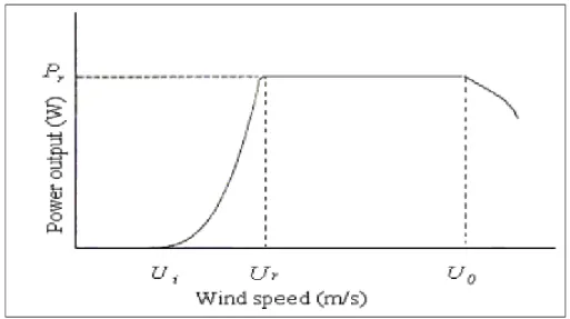
The power curve of the wind turbine is a diagram that depicts the power generation of a wind turbine at various wind speeds. The wind turbine will measure the energy output without taking the technological details of its various components into consideration with such a curve. Based on the hub height wind speed, the power curve provides the energy production [34]. The power curves are obtained using structured

approximation for the power curve for a given machine. The following parameter is seen in the figure (3.1) as an example of a power curve for the standard wind turbine:

• Speed of cut-in, the wind speed at which the turbine begins generating electricity.

• The amount of wind velocity exceeds rated turbine strength at the turbine. Often this is the maximum strength, but not always.

• The cut-off wind speed is that of the wind turbine, which ceases output and flows away from the main wind stream. The cutting wind speed is usually between 20 and 25 m/s [35].

Figure 3.1. Power output from wind turbine as function of wind speed.

3.11.2. Annual Energy Production

Annual energy output calculations are highly significant in the estimation of any wind energy project. In accordance with the power curve of a single wind turbine the longer long-term wind speed distribution provides the energy produced with any wind velocity and therefore overall energy generated over the year. The statistical representation of annual energy generation (AEP) is as follows [36]. The probability that a wind speed 𝑣0 will fall between two wind speeds 𝑣𝑖 and 𝑣𝑖+1 is obtained from

𝐹(𝑣_𝑖 < 𝑣₀ < 𝑣_𝑖+1) = 𝑒𝑥𝑝 [− (𝑣𝑖 𝑐) 𝑘 ] − 𝑒𝑥𝑝 [− (𝑣𝑖+1 𝑐 ) 𝑘 ] (3.20)

The total annual energy production is calculated as:

𝐴𝐸𝑃 = ∑1 2[𝑃(𝑣𝑖+1) + 𝑃(𝑣𝑖)] 𝑁−1 𝑖=1 ∙ 𝐹(𝑣_𝑖 < 𝑣₀ < 𝑣_𝑖+1) ∙ 8760 (3.21)

Where, 𝑃(𝑣𝑖) is the power output of a certain wind turbine at wind speed 𝑣𝑖 and 8760

is the number of hours in the year.

3.11.3. Availability

The availability in a wind turbine to produce electricity is the fraction of the time in a year. Include down periods for routine repairs or unplanned repair when the wind turbine is no longer accessible. The typical availabilities for modern wind turbines are 95-99 (%) better than many items of conventional generating plant.

Useful electricity is provided only during cuts and cuts in wind speeds, and the turbine can run at a degree different to its availability due to wind conditions. Depending on wind conditions. A further calculation is that if the machinery was operating at its rate of efficiency all year long (8760 hours), the capacity factor (Cf) is specified as the proportion of the real annual energy production to the theoretical high output. Factor of capability, computed as [34].

𝐶𝑓 =𝑎𝑐𝑡𝑢𝑎𝑙 𝑒𝑛𝑒𝑟𝑔𝑦 𝑜𝑢𝑡𝑝𝑢𝑡(𝑘𝑤ℎ)

𝑟𝑎𝑡𝑒𝑑 𝑐𝑝𝑎𝑐𝑖𝑡𝑦 (𝑘𝑤) × 8760 × 100

(3.22)

Related power plant output metrics exist. The accurate definition of availability or load factor should be well understood to prevent uncertainty in comparing the wind turbine output.

3.12. PRESENT VALUE COST AND ELECTRICITY PRICE

To calculate the present value cost, PVC, the values of the different terms in Eq. (3.23) should be known. In this study those values have been calculated based on the values in [10,11,12]. 𝑃𝑉𝐶 = 𝐼 + 𝐶_𝑜𝑚𝑟[1 + 𝑖 𝑟 − 𝑖] × [1 − [ 1 + 𝑖 1 + 𝑟] 𝑡 ] − 𝑆 [1 + 𝑖 1 + 𝑟] 𝑡 _(3.23)

The cost of each kWh produced by the turbine in, USD cent/kWh, is calculated from Eq. (3.24).

𝐾𝑊ℎ 𝑝𝑟𝑖𝑐𝑒 = 𝑃𝑉𝐶

𝐴𝐸𝑃 × 𝑇× 100

(3.24)

3.13. GREENHOUSE GASES EMISSION REDUCTION

GHG reduction is calculated from Eq. (3.25).

ΔGHG = (ebase − eprop) Eprop (1 − λprop) (1 − ecr) (3.25)

Where,

𝑒𝑏𝑎 : is the base case GHG emission factor (tCO2/MWh). 𝑒𝑝𝑟𝑜𝑝: is the proposed case GHG emission factor (tCO2/MWh)

𝐸𝑝𝑟𝑜𝑝: is the annual electricity produced by the wind turbine in the different sites calculated previously. (MWh).

𝜆𝑝𝑟𝑜𝑝: is the fraction of the electricity loss in transmission and distribution (T&D

losses) for the proposed case.

So, the new price:

𝐾𝑊ℎ 𝐶𝑜𝑠𝑡 =𝑃𝑉𝐶 𝑤𝑖𝑡ℎ𝑜𝑢𝑡 𝐺𝐻𝐺 − 𝑝𝑟𝑖𝑐𝑒 𝑜𝑓 𝑎𝑛𝑛𝑢𝑎𝑙 𝐺𝐻𝐺 𝑟𝑒𝑑 × 𝑡

𝐴𝐸𝑃 × 𝑡 х 100

(3.26)

PART 4

RESULT

In this study, technical and economic assessments for three different cities located close to the Libyan coast have been conducted and the fourth site located in the south. The site, Adirsiyah, is located in the eastern side of the coast where the other two sites, Espiaa and Msallata, are located in the western side of the coast and the Alqatrun site located in the south. Three separate approaches were used in the estimation of Weibull parameters; visual method, empiric method and highest probability method. The Weibull distribution results obtained from each method were fitted against the actual data. Error analysis by calculating the Determination of coefficient (R2), root mean square error (RMSE), mean bias error (MBE) and mean bias absolute error (MAE) is also done to check for the validity of the computed Weibull distributions. The technological appraisal includes estimation, power factor and greenhouse gas emissions reduction annual energy generation (GHG). While the economic assessment includes cost analysis for the produced electricity in $ cent/kWh and the calculation of the GHG reduction income and its effect on the produced electricity cost. The effects of different Weibull parameters on the analysis are also addressed in this study.

4.1. WIND DATA

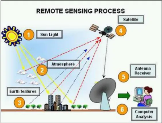
In determining and using wind tools, knowledge of the characteristics of the wind regimes in any position is significant. Figure 4.1 demonstrates the latest analysis to test wind energy in four different areas. The data were collected from the Weather Authority and the National Agency for the Atmosphere and Resources of Libya.

Figure 4.1. Location of sites.

Table 4.1. Physical features of the meteorological stations.

Station (Site) Latitude Longitude Altitude (m) Msallata 32.5836o N 14.0363o E 198 m Espiaa 32.5457o N 13.1683o E 156 m Alqatrun 24.9333o N 14.6333o E 518 m Adirsiyah 32.7013o N 20.9417o E 332 m

The real wind data measured at 20 and 60m height is used in this investigation. The average wind velocity 𝑉𝑚 is the most common wind power measure. Averages of estimated wind speeds at each site are seen in Tables (4.2), (4.3) each month and every year. From this table, a maximum average value of 10.9 m/s was recorded at Msallata in April while a minimum average value of 3.1 m/s was measured Adirsiyah in August.

Table 4.2. Average wind speeds (20m).

Site

Monthly Average Wind Speeds (m/s) Annual

Averages January February March April May June July August September October November December (m/s) Espiaa 5.489 6.69 6.56 7.55 5.78 6.2 4.67 5.48 4.98 6.12 6.01 6.118 5.97 Msallata 5.59 7.2 6.69 9.58 6.8 7.35 6.0 6.36 6.37 7.01 6.11 5.58 6.72 Alqatrun 5.1 6.47 6.08 6.98 5.53 5.32 4.09 3.46 4.47 6.25 5.36 5.48 5.382 Adirsiyah 6 5.01 5.03 5.44 3.69 3.37 3.02 3.01 4.46 4.12 5.04 6.25 4.537

Table 4.3. Average wind speeds (60m).

Site

Monthly Average Wind Speeds (m/s) Annual

Averages (m/s) January February March April May June July August September October November December

Espiaa 6.59 7.89 8.17 9.49 7.41 7.87 6.49 6.99 6.45 7.46 7.11 7.3 7.436 Msallata 6.69 8.78 8.34 10.9 8.48 9.01 7.42 7.78 7.82 8.46 7.29 6.667 8.136 Alqatrun 6.39 8.02 6.75 8.96 7.19 6.28 4.77 3.88 5.01 7.66 6.46 6.79 6.5055 Adirsiyah 7.28 5.64 6.01 6.32 4.29 3.7 3.4 3.1 5.01 4.85 6.03 7.48 5.258

Figures (4.2), (4.3) show a comparison of the monthly mean wind speeds between the sites. The figure shows that Msallata and Espiaa have the highest mean wind speeds along the year and their highest wind speeds were recorded in April. Adirsiyah, on the other hand, has the lowest wind rates in the year relative to the other locations.

Figure 4.2. Monthly variation of wind speeds for the selected sites (20m).

Figure 4.3. Monthly variation of wind speeds for the selected sites (60m).

2 4 6 8 10 12 0 1 2 3 4 5 6 7 8 9 10 11 12 M o n th ly M e an Wi n d Sp e e d ( m /s) Months

Masllata Espiaa Adirsiyah Alqatrun

2 4 6 8 10 12 14 0 1 2 3 4 5 6 7 8 9 10 11 12 M o n th ly M e an Wi n d Sp e e d ( m /s) Months

From this point after, the measurements that will be considered for further investigations are the ones correspond to 20m and 60m height. The annual mean wind speeds for the different sites at 20m and 60m heights are shown below:

Figure 4.4. Annual mean wind speeds for the selected sites at 20m height.

Figure 4.5. Annual mean wind speeds for the selected sites at 60m height.

The measured annual wind speed frequency curves are plotted for all the sites in Figure (4.6). From Figure (4.7) we notice that the distribution curves of the sites have similar trends. They increase to reach a peak value and decrease after that. The peak amount is near to the annual average site speed. The peak value of the frequency ranges between 11 % and 17 %. 0 1 2 3 4 5 6 7 8

Adirsiyah Alqatrun Espiaa Masllata

An n u al Av era ge Win d Sp ee d (m /s ) 0 1 2 3 4 5 6 7 8 9

Adirsiyah Alqatrun Espiaa Masllata

A n n u al Av e rag e Wi n d Sp e e d (m /s)

Figure 4.6. Measured annual frequency distribution (20m).

Figure 4.7. Measured annual frequency distribution (60m).

4.2. WEIBULL PARAMETERS

The Weibull parameters are calculated using the three different methods mentioned before. The results corresponding to the graphical method for each site are obtained from the plots shown in Figures 4.8, 4.9. The Weibull parameters results for the different sites calculated from the different methods are shown in Table 4.3. The results obtained in Table 4.3 show that there are differences among the, k, and, c, values obtained by the different methods. MLM method results in higher values for the Weibull parameters for all the sites studied while the GM method results in lower values for the Weibull parameters. This difference in the results will affects the

0 5 10 15 20 -2 0 2 4 6 8 10 12 14 16 18 20 22 24 26 28 30 32 34 Fr e q u an cy %

Mean Wind Speed (m/s)

Alqatrun Adirsiyah Masllata Espiaa 0 5 10 15 20 -2 0 2 4 6 8 10 12 14 16 18 20 22 24 26 28 30 32 34 Fr e q u an cy %

Mean Wind Speed (m/s)

Alqatrun Adirsiyah

Figure 4.8. Graphical method to estimate the Weibull parameters at 20m. y = 2.2161x - 4.5959 R2 _{= 0.99005} -6 -5 -4 -3 -2 -1 0 1 2 3 0 1 2 3 4 ln( -l n( 1 -F (v )) ) ln v Msallata y = 1.5001x - 2.6298 R2_{= 0.96964} -3 -2 -1 0 1 2 3 4 0 1 2 3 4 ln( -l n( 1 -F (v )) ) ln v Alqatrun y = 1.5849x - 2.5337 R² = 0.99483 -3 -2 -1 0 1 2 3 0 1 2 3 4 ln( -l n( 1 -F (v )) ) ln v Adirsiyah y = 1.7987x - 3.5171 R² = 0.99843 -5 -4 -3 -2 -1 0 1 2 3 0 1 2 3 4 ln( -l n( 1 -F (v )) ) ln v Espiaa

Figure 4.9. Graphical method to estimate the Weibull parameters at 60m. y = 1.8921x - 4.1637 R² = 0.99778 -6 -5 -4 -3 -2 -1 0 1 2 3 0 1 2 3 4 ln( -l n( 1 -F (v )) ) ln v Espiaa y = 2.2878x - 5.2139 R² = 0.99817 -6 -5 -4 -3 -2 -1 0 1 2 3 0 1 2 3 4 ln( -l n( 1 -F (v )) ) ln v Msallata y = 1.8067x - 3.5284 R² = 0.99345 -5 -4 -3 -2 -1 0 1 2 3 0 1 2 3 4 ln( -l n( 1 -F (v )) ) ln v Alqatrun y = 1.4077x - 2.2965 R² = 0.99421 -3 -2 -1 0 1 2 3 4 0 1 2 3 4 ln( -l n( 1 -F (v )) ) ln v Adirsiyah

Table 4.4. Weibull Parameters estimated by three different 20m.

Table 4.5. Weibull Parameters estimated by three different 60m.

4.3. PROBABILITY DENSITY AND CUMULATIVE DISTRIBUTION FUNCTION

By replacing the Weibull parameters (k and c) in equations 3.8 and 3.7, the probability density function and cumulative distribution function are determined. The density of probability function corresponds to the wind blowing frequency at some rate. The calculated probability density function using Weibull parameters computed from different methods are fitted against the frequency of the actual wind data in Fig. 4.9 and 4.10 show that for the sites were the wind speed is low (Adirsiyah and Alqatrun)

Site Methods GM EM MLM 𝑘 𝑐 𝑘 𝑐 𝑘 𝑐 Msallata 2.2161 7.9562 2.341 8.172 2.552 8.344 Espiaa 1.7987 7.0664 2.215 7.224 2.223 7.515 Alqatrun 1.5001 5.7665 1.613 6.625 1.721 6.763 Adirsiyah 1.5849 4.9481 1.672 5.076 2.094 5.634 Site Methods GM EM MLM 𝑘 𝑐 𝑘 𝑐 𝑘 𝑐 Msallata 2.2878 9.7733 2.423 9.814 2.643 10.020 Espiaa 1.8921 9.0298 2.045 9.024 2.290 9.185 Alqatrun 1.8067 7.0533 1.981 7.282 2.214 7.491 Adirsiyah 1.4077 5.1134 1.435 5.750 1.721 6.094

Msallata), where the wind speed is high, it is noticed that the computed probability density function matches well with the actual data for all the used methods with the MLM giving better agreement with the actual data for all the sites.

Figure 4.10. Comparison of the probability density function 20m.

0 2 4 6 8 10 12 14 0 5 10 15 20 25 Pr o b ab ili ty D e n si ty Fu n ction % Wind Speed (m/s) Espiaa GM EM MLM Actual 0 2 4 6 8 10 12 14 0 5 10 15 20 25 Pr o b ab ili ty D e n si ty Fu n ction % Wind Speed (m/s) Msallata GM EM MLM Actual 0 2 4 6 8 10 12 14 0 5 10 15 20 25 Pr o b ab ili ty D e n si ty Fu n ction % Wind Speed (m/s) Alqatrun GM EM MLM Actual 0 2 4 6 8 10 12 14 16 18 20 0 5 10 15 20 25 P rob abil ity D en si ty Fun ct ion % Wind Speed (m/s) GM EM MLM Actual Adirsiyah

Figure 4.11. Comparison of the probability density function 60m. 0 2 4 6 8 10 12 14 0 5 10 15 20 25 Pr o b ab ili ty D e n si ty Fu n ction % Wind Speed (m/s) Espiaa GM EM MLM Actual 0 2 4 6 8 10 12 14 0 5 10 15 20 25 Pr o b ab ili ty D e n si ty Fu n ction % Wind Speed (m/s) Msallata GM EM MLM Actual 0 2 4 6 8 10 12 14 0 5 10 15 20 25 P rob abil ity D en si ty Fun ct ion % Wind Speed (m/s) Alqatrun GM EM MLM Actual 0 2 4 6 8 10 12 14 16 18 0 10 20 30 Pr o b ab ili ty D e n si ty F u n cti o n % Wind Speed (m/s) GM EM MLM Actual Data Adirsiyah

Figure 4.12. Cumulative distribution function for the sites at 20m height. 0 0.2 0.4 0.6 0.8 1 1.2 0 5 10 15 20 25 30 C u mu lati ve D istr ib u ti o n F u n cti o n Wind Speed (m/s) Msallata GM EM MLM Actual Data 0 0.2 0.4 0.6 0.8 1 1.2 0 5 10 15 20 25 30 C um ul at iv e D is tr ibut ion f unct ion Wind Speed (m/s) Alqatrun GM EM MLM Actual Data 0 0.2 0.4 0.6 0.8 1 1.2 0 5 10 15 20 25 30 C u mu latı ve D ıtr ıb u tı o n F u n ctı o n Wind Speed (m/s) Espiaa GM EM MLM Actual 0 0.2 0.4 0.6 0.8 1 1.2 0 5 10 15 20 25 30 C u mu latı ve D ıstr ıb u tı o n F u n ctı o n Wind Speed (m/s) Adırsıyah GM EM MLM Actual Data

Figure 4.13. Cumulative distribution function for the sites at 60m height.

4.4. ERROR ANALYSIS RESULTS

The errors associated with the different Weibull methods are calculated using equations 11-14 and the error results are shown in Table 4.6 and 4.7. The small values for RSME, MBE and MAE verifies that the methods for calculating the Weibull parameters in this study are accurate and can be used for wind energy assessment. Also the R2 values are close to 1.0 for all the methods in all the sites which proves the

0 0.2 0.4 0.6 0.8 1 1.2 0 5 10 15 20 25 30 C u mu lati ve D istr ib u ti o n F u n cti o n Wind Speed (m/s) Msallata GM EM MLM Actual Data 0 0.2 0.4 0.6 0.8 1 1.2 0 5 10 15 20 25 30 C um ul at iv e D is tr ibut ion f unct ion Wind Speed (m/s) Alqatrun GM EM MLM Actual 0 0.2 0.4 0.6 0.8 1 1.2 0 5 10 15 20 25 30 C u mu latı ve D ıstr ıb u tı o n F u n ctı o n Wind Speed (m/s) Espiaa GM EM MLM Actual 0 0.2 0.4 0.6 0.8 1 1.2 0 5 10 15 20 25 30 C u mu latı ve D ıstr ıb u tı o n F u n ctı o n Wind Speed (m/s) Adırsıyah GM EM MLM Actual