Short-Time Fourier Transform: Two Fundamental
Properties and an Optimal Implementation
Lütfiye Durak, Student Member, IEEE, and Orhan Arıkan, Member, IEEE
Abstract—Shift and rotation invariance properties of linear time-frequency representations are investigated. It is shown that among all linear time-frequency representations, only the short-time Fourier transform (STFT) family with the Her-mite–Gaussian kernels satisfies both the shift invariance and rotation invariance properties that are satisfied by the Wigner distribution (WD). By extending the time-bandwidth product (TBP) concept to fractional Fourier domains, a generalized time-bandwidth product (GTBP) is defined. For mono-component signals, it is shown that GTBP provides a rotation independent measure of compactness. Similar to the TBP optimal STFT, the GTBP optimal STFT that causes the least amount of increase in the GTBP of the signal is obtained. Finally, a linear canonical decomposition of the obtained GTBP optimal STFT analysis is presented to identify its relation to the rotationally invariant STFT.
Index Terms—Fractional Fourier transform, generalized time-bandwidth product, linear time-frequency representations, rota-tion invariance, short-time Fourier transform.
I. INTRODUCTION
R
ESEARCH on time-frequency domain characterization of signals has been focused on the variants of short-time Fourier transform (STFT) [1]–[7] and Wigner distribution (WD) [8], [9]. The absence of undesirable cross terms [1], [10] and computational simplicity [11]–[13] are the major factors in the wide-spread use of the STFT in practice. With the advance of faster processors, the efficiency of the STFT techniques have become less important. However, the ability of representing time-frequency content of signals free of cross terms is still the major advantage of the STFT techniques over the WD-related quadratic time-frequency distributions.Among its many important properties, the STFT has a fun-damental property that simplifies the interpretation of the resul-tant distribution: magnitude-wise shift invariance in both time and frequency. In this paper, we first prove that the STFT is the only linear distribution that has the magnitude-wise shift in-variance property in both time and frequency. Then, we investi-gate time-frequency domain rotation property within the general class of linear distributions. This lesser known property, which is satisfied by the WD, is defined as follows: A time-frequency distribution satisfies the rotation property if the distribution of an arbitrary signal and the distribution of its th-order fractional
Manuscript received August 28, 2001; revised October 23, 2002. The asso-ciate editor coordinating the review of this paper and approving it for publication was Prof. Paulo S. R. Diniz.
The authors are with the Department of Electrical Engineering, Bilkent University, Ankara, Turkey (e-mail: [email protected]; [email protected]).
Digital Object Identifier 10.1109/TSP.2003.810293
Fourier transformation are rad rotated versions of each other [14], [15]. We start our investigation on linear time-fre-quency distributions by showing that STFT satisfies the rota-tion property only if the STFT kernel is a Hermite-Gaussian function. Thus, we reach the conclusion that the linear time-fre-quency distributions, which satisfy both the rotation property and the magnitude-wise time and frequency shift property, are the STFT with Hermite-Gaussian kernels.
The choice of the STFT kernel determines the time-frequency signal localization properties of the distribution. Among the Hermite-Gaussian function family, since it has the minimum time-bandwidth product (TBP), the Gaussian function is the most commonly used kernel function. However, STFT with the Gaussian kernel still suffers from the problem of limited resolution. To overcome the inherent tradeoff between the time and the frequency localization of the STFT, several alternatives have been investigated in the literature. In [5], using two kernel functions of different supports, a wideband and a narrowband spectrogram are obtained. In order to preserve the localization characteristics of both, a combined spectrogram is formed by computing the geometric mean of the corresponding STFT magnitudes, whereas in [6], the STFT is evaluated by using a kernel function with an adaptive width in order to analyze the transient response of radar targets. In [16], a kernel matching algorithm is developed by locally adapting the Gaussian kernel functions to the analyzed signal. Although these investigations provide significant improvements in the time-frequency lo-calization of signal components, in the presence of chirp-like signals, they still provide descriptions whose localization prop-erties depends on the chirp rate of the components. Recently, [7] introduced an improved instantaneous frequency estimation technique using an adaptive STFT where the kernel functions are chosen from a set of functions through adaptation rules and computation of the STFT with varying kernel functions at each time instance. In addition, apart from the analysis of de-terministic signals, there have been studies where time-varying spectra of random processes are investigated [17].
In this paper, we characterize the time-frequency domain lo-calization by STFT and investigate the effect of the STFT kernel on the obtained time-frequency representation of signals. We in-troduce the generalized time-bandwidth product (GTBP) defini-tion to provide a rotadefini-tion-invariant measure of signal support in the time-frequency domain. Then, we obtain the optimal STFT kernel that provides the most compact representation consid-ering the GTBP of a signal component. The proposed time-fre-quency analysis is shown to be equivalent to an ordinary STFT analysis conducted in a scaled fractional Fourier transform do-main. The obtained GTBP optimal STFT representation yields 1053-587X/03$17.00 © 2003 IEEE
optimally compact time-frequency supports for chirp-like sig-nals on the STFT plane. In general, the GTBP optimal STFT representation does not satisfy the rotation property. However, as shown in detail, there exists a linear canonical decomposition of the GTBP optimal STFT that provides the link between the GTBP optimal STFT and the rotation invariance property.
This paper is organized as follows. In Section II, we show that the STFT is the only linear time-frequency representation that satisfies the magnitude-wise shift invariance property. In Section III, we define the rotation property of shift-invariant time-frequency distributions and obtain the class of STFT ker-nels satisfying the rotation property. In Section IV, we introduce the GTBP and obtain the GTBP optimal STFT kernel. In Sec-tion V, we present a linear canonical decomposiSec-tion of the GTBP optimal STFT and relate it to the rotation property. Furthermore, the performance of the GTBP optimal STFT representation is il-lustrated by using simulated data. Finally, the paper is concluded in Section VI with future research directions.
II. LINEAR SHIFT-INVARIANT TIME-FREQUENCYDISTRIBUTIONS
Time-frequency distributions are designed to characterize the time-frequency content of signals. Since time or frequency shifts do not change the time-frequency content of a signal, except to relocate it correspondingly, it is important that time-frequency representations satisfy the magnitude-wise shift invariance property. A precise statement of this property is given as follows: A time-frequency representation is magnitude-wise shift invariant if for
(1) In this section, we investigate the magnitude-wise shift invari-ance property within the class of linear time-frequency repre-sentations.
The magnitude-wise shift invariance of linear time-frequency distributions can be characterized fully as follows. The gen-eral kernel-based form of a linear time-frequency distribution
is given by1
(2) where is the kernel of the distribution [18]. By making use of the general theorem on linear systems given in Appendix A, it can be shown easily that the magnitude-wise shift invariance in time requires to have the following form:
(3) Since the magnitude of time-frequency distributions are related to the energy distribution of the signals in the time-frequency plane, will be ignored in the rest of the derivations. The
1All integrals are from01 to +1 unless otherwise stated.
implications of magnitude-wise shift invariance in frequency can be investigated in the Fourier domain as
(4) where is the Fourier transform of , and . The magnitude-wise shift invariance with respect to frequency requires that
(5) Thus, the kernel has the following representation:
(6) Since the phase and can be ignored, the general form of a magnitude-wise shift invariant linear time-frequency distribution is
(7) which has the same form of the STFT [1], [3] with the kernel . Consequently, STFT is the only distribution that is linear and magnitude-wise shift-invariant under both time and frequency shifts.
III. LINEARTIME-FREQUENCYDISTRIBUTIONS AND THEROTATIONPROPERTY
The lesser known rotation property of time-frequency distri-butions is defined as follows:
Definition 1: A time-frequency distribution satis-fies the rotation property [19] if for all and
(8) where is equal to , and is the th-order fractional Fourier transformation (FrFT) of given by [20], [21]
(9)
where is
(10) and the rotation operator acting on a two-dimensional (2-D) function is defined as
(11) It has been shown that a quadratic time-frequency distribu-tion satisfies the rotadistribu-tion property only if it has a rotadistribu-tionally
symmetric kernel [22]. The most widely known quadratic dis-tribution satisfying the rotation property is the WD
(12) where is the WD of [14], [15], [19]. As the time and frequency variables have different units, a dimensional normalization of the time-frequency plane is required before performing the rotation operation [23]. It is assumed that the time and frequency domain representations of a signal are
confined to [ ] and [ ] intervals,
respectively. Then, a scaling parameter is introduced, where the dimension of time and scaled coordinates and are used as new coordinates. This way, the time and frequency representations of the signal are confined to intervals of length and . We choose so that the lengths of both intervals are equal to , which is a dimensionless quantity. In numerical examples, signals can be represented in both domains with samples spaced apart. In the paper, we assume that a dimensional normalization has already been done and all the coordinates represent dimension-less quantities.
The rotation property has some important conceptual and practical implications [14], [15], [24]–[27]. It implies that the inherent time-frequency domain characteristics of a signal remains unchanged in all the fractional Fourier domains. Therefore, there is nothing special about any of the fractional Fourier domain representations of a signal including the commonly used time or frequency domains. Among the linear, shift-invariant time-frequency distributions, only the STFT with Hermite-Gaussian kernels satisfies the rotation property. This can be shown as follows:
Proposition 1: STFT satisfies the rotation property only if
the window function is a Hermite-Gaussian function.
Proof: The STFT of the fractionally Fourier transformed
is
STFT (13)
By using (9) and the property [21], we
obtain STFT
(14)
where . The rotation
prop-erty requires that the magnitude of (13) is equal to the magnitude of STFT , which imposes the following condition on
to hold true for all
(15)
where does not depend on but may be a function of . The equality in (15) can only be satisfied if is one of the eigen-functions of the FrFT operator. The Hermite-Gaussian eigen-functions form the complete set of eigenfunctions of the FrFT operator de-fined in (9) [21]. Then, will be the eigenvalue of the FrFT such that equals , where is the Hermite polynomial order.
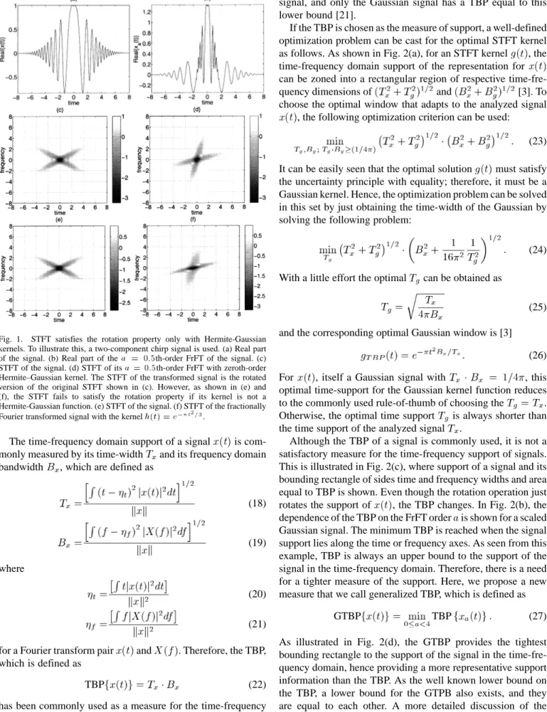
The rotation property of the STFT with the zeroth-order Her-mite-Gaussian kernel is illustrated in Fig. 1(c) and (d), which corresponds to the STFT of the time domain signal and the 0.5th-order fractionally Fourier transformed signal in Fig. 1(a) and (b), respectively. The rotation property fails if the STFT of both of these signals are computed with a scaled Gaussian window function, as shown in Fig. 1(e) and (f) .
It will be shown next that the rotation property fails when the STFT kernel is a linear combination of many Hermite–Gaussian functions.
Proposition 2: The rotation property fails when the STFT
kernel is a linear combination of Hermite–Gaussian functions.
Proof: The Hermite–Gaussian functions are the
eigen-functions of the FrFT. For each FrFT order
(16) where is the th-order Hermite–Gaussian function, and . If is a combination of Hermite–Gaussian
functions as with arbitrary nonzero
coefficients, then on the left-hand side of (15) is
(17)
The condition in (15) requires (17) be equal to . However, for arbitrary , if , then . Therefore, any linear combination of Hermite–Gaussian functions fails to satisfy the rotation property of STFT.
IV. TIME-FREQUENCYDOMAINLOCALIZATION BYSTFT An important criterion for the success of time-frequency rep-resentations is how well it preserves the time-frequency domain support of signals. Among the commonly used time-frequency representations, WD is the best in this respect. However, the cross-terms of the WD clutters the obtained time-frequency rep-resentation. Therefore, in a way, it disturbs the actual support of the signal in the time-frequency domain. The STFT family pro-vides cross-term free time-frequency representations. So, sup-port preservation criteria is applicable to measure the success of the alternative STFT representations. In this section, we in-vestigate the effect of the STFT kernel on the obtained time-fre-quency support of the signal components. This investigation will require generalized definition of the time-bandwidth product. Furthermore, it will lead to signal adaptive STFTs.
Fig. 1. STFT satisfies the rotation property only with Hermite-Gaussian kernels. To illustrate this, a two-component chirp signal is used. (a) Real part of the signal. (b) Real part of thea = 0:5th-order FrFT of the signal. (c) STFT of the signal. (d) STFT of itsa = 0:5th-order FrFT with zeroth-order Hermite–Gaussian kernel. The STFT of the transformed signal is the rotated version of the original STFT shown in (c). However, as shown in (e) and (f), the STFT fails to satisfy the rotation property if its kernel is not a Hermite-Gaussian function. (e) STFT of the signal. (f) STFT of the fractionally Fourier transformed signal with the kernelh(t) = e .
The time-frequency domain support of a signal is com-monly measured by its time-width and its frequency domain bandwidth , which are defined as
(18)
(19) where
(20)
(21) for a Fourier transform pair and . Therefore, the TBP, which is defined as
TBP (22)
has been commonly used as a measure for the time-frequency domain support of the signal. The well-known uncertainty prin-ciple dictates that is a lower bound on the TBP of a
signal, and only the Gaussian signal has a TBP equal to this lower bound [21].
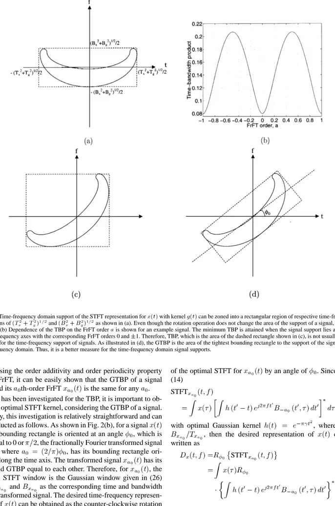
If the TBP is chosen as the measure of support, a well-defined optimization problem can be cast for the optimal STFT kernel as follows. As shown in Fig. 2(a), for an STFT kernel , the time-frequency domain support of the representation for can be zoned into a rectangular region of respective
time-fre-quency dimensions of and [3]. To
choose the optimal window that adapts to the analyzed signal , the following optimization criterion can be used:
(23) It can be easily seen that the optimal solution must satisfy the uncertainty principle with equality; therefore, it must be a Gaussian kernel. Hence, the optimization problem can be solved in this set by just obtaining the time-width of the Gaussian by solving the following problem:
(24) With a little effort the optimal can be obtained as
(25) and the corresponding optimal Gaussian window is [3]
(26) For , itself a Gaussian signal with , this optimal time-support for the Gaussian kernel function reduces to the commonly used rule-of-thumb of choosing the . Otherwise, the optimal time support is always shorter than the time support of the analyzed signal .
Although the TBP of a signal is commonly used, it is not a satisfactory measure for the time-frequency support of signals. This is illustrated in Fig. 2(c), where support of a signal and its bounding rectangle of sides time and frequency widths and area equal to TBP is shown. Even though the rotation operation just rotates the support of , the TBP changes. In Fig. 2(b), the dependence of the TBP on the FrFT order is shown for a scaled Gaussian signal. The minimum TBP is reached when the signal support lies along the time or frequency axes. As seen from this example, TBP is always an upper bound to the support of the signal in the time-frequency domain. Therefore, there is a need for a tighter measure of the support. Here, we propose a new measure that we call generalized TBP, which is defined as
GTBP TBP (27)
As illustrated in Fig. 2(d), the GTBP provides the tightest bounding rectangle to the support of the signal in the time-fre-quency domain, hence providing a more representative support information than the TBP. As the well known lower bound on the TBP, a lower bound for the GTPB also exists, and they are equal to each other. A more detailed discussion of the uncertainty relationship in the fractional Fourier domains can be found in [28]–[31].
Fig. 2. Time-frequency domain support of the STFT representation forx(t) with kernel g(t) can be zoned into a rectangular region of respective time-frequency dimensions of(T + T ) and(B + B ) as shown in (a). Even though the rotation operation does not change the area of the support of a signal, the TBP changes. (b) Dependence of the TBP on the FrFT ordera is shown for an example signal. The minimum TBP is attained when the signal support lies along the time or frequency axes with the corresponding FrFT orders 0 and61. Therefore, TBP, which is the area of the dashed rectangle shown in (c), is not usually a tight measure for the time-frequency support of signals. As illustrated in (d), the GTBP is the area of the tightest bounding rectangle to the support of the signal in the time-frequency domain. Thus, it is a better measure for the time-frequency domain signal supports.
By using the order additivity and order periodicity property of the FrFT, it can be easily shown that the GTBP of a signal
and its th-order FrFT is the same for any . As it has been investigated for the TBP, it is important to ob-tain the optimal STFT kernel, considering the GTBP of a signal. Actually, this investigation is relatively straightforward and can be conducted as follows. As shown in Fig. 2(b), for a signal whose bounding rectangle is oriented at an angle , which is not equal to 0 or , the fractionally Fourier transformed signal , where , has its bounding rectangle ori-ented along the time axis. The transformed signal has its TBP and GTBP equal to each other. Therefore, for , the optimal STFT window is the Gaussian window given in (26) with and as the corresponding time and bandwidth of the transformed signal. The desired time-frequency represen-tation of can be obtained as the counter-clockwise rotation
of the optimal STFT for by an angle of . Since, as in (14)
STFT
(28) with optimal Gaussian kernel , where
, then the desired representation of can be written as
STFT (29a)
In (29b), the expression in the brackets can be recognized as the th-order FrFT of , which is simply the time and frequency shifted form of the kernel . Using the time and frequency shift properties of the FrFT, D is computed as
(30)
where , and the optimal
kernel is
(31)
where . Since the phase
can be ignored in , it is easy to see that the de-sired representation in (30) has the form of STFT with kernel . This explicit form of the GTBP optimal STFT dis-tribution provides significant computational saving in practice. Once the fractional order is determined, the computational complexity of (30) is the same as the computational complexity of the ordinary STFT. The discrete STFT is defined as [1]
STFT
(32) where and are integers, and and are the sampling inter-vals of time and frequency, and it can be efficiently implemented by using FFT techniques.
There are many alternative approaches to determine the op-timal fractional order to be used in the GTBP optimal STFT analysis. Since the optimal fractional order corresponding to a signal and its orientation in the time-frequency plane are related, the optimal order can be estimated by determining the orientation of the signal in the time-frequency plane. One way of determining the orientation of a signal in the time-frequency plane is to search for the peaks in the FrFT magnitudes com-puted at various fractional orders [14], [32], [33]. In practice, the search for the optimal fractional order can be conducted approximately by computing the FrFT of the signal at ten to 30 different fractional orders. Since each FrFT computation is , the overall complexity of the required search is of as well. The FrFT computation algorithm is given in Table I [23], [27]. Alternatively, for mono-component signals, the required fractional Fourier transformation order can also be found based on the fractional moments of the signal. Efficient ways of computing the fractional Fourier transform moments of a signal are given in [34] and [35]. In addition, for signals with strong harmonics, an alternative mean of determining the required fractional Fourier transformation order can be found in
[36]. In practical applications, both the orientation angle of the signal and parameters related to the dimensions of the bounding rectangle in the appropriate fractional Fourier domain should be adaptively chosen. As future work, the performances of alterna-tive ways of determining these parameters can be compared.
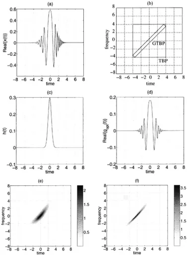
In Fig. 3, time-frequency domain localization by TBP op-timal STFT and GTBP opop-timal STFT of a quadratic FM signal shown in Fig. 3(a) is com-pared. The STFTs are evaluated with the kernels determined by using (26) and (31), as shown in Fig. 3(c) and (d), respectively. Time-frequency support of the GTBP optimal STFT illustrated in Fig. 3(f) is significantly better localized when compared with the TBP optimal STFT illustrated in Fig. 3(e).
The GTBP optimal STFT in (30) does not possess the rotation property because is not a member of the Hermite–Gaussian function family; however, it has an envelope that is a scaled zeroth-order Hermite–Gaussian function. If the scaling is not equal to 1, the rotation property cannot be satisfied. In the next section, we will provide a canonical decomposition of GTBP optimal STFT such that the rotation invariance is satisfied in a certain scaled fractional Fourier domain.
V. GTBP OPTIMALSTFTANDROTATIONPROPERTY In Section IV, we have demonstrated that GTBP optimal STFT can be evaluated as efficiently as ordinary STFT. Using (30) and (31), the GTBP optimal STFT of a signal with a support oriented at an angle of with respect to the time axis in the time-frequency plane is as in (33), shown at the bottom of the page.
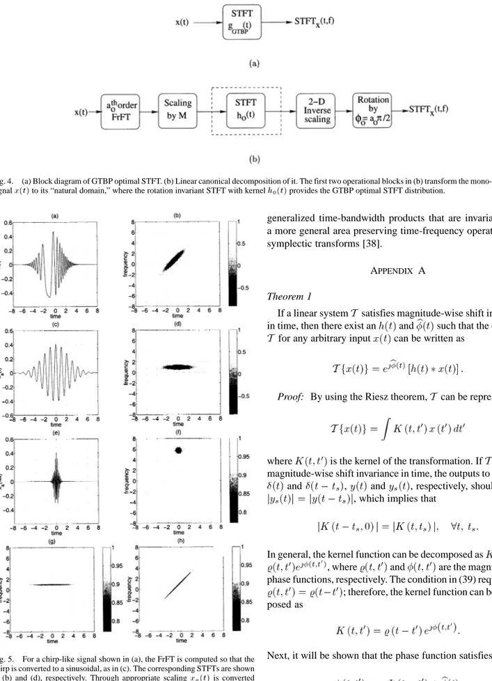
Although (33) provides an efficient implementation method for the GTBP optimal STFT analysis, we would like to introduce a multistage implementation of it, as shown in Fig. 4(b), with its explicit derivation detailed in Appendix B. This decomposition is a linear canonical representation of the GTBP optimal STFT analysis with a sequence of operations explained and illustrated in Fig. 5. First, the th-order FrFT of the input signal is com-puted using (9). As shown in Fig. 5(d), the time-frequency sup-port of the transformed signal [which is shown in Fig. 5(c)] is oriented along the time axis.
After this operation, the major axis of the time-frequency do-main support of the transformed signal is along the time axis. Hence, the conventional TBP provides a good support informa-tion on the transformed signal. Assuming that the time and fre-quency widths of the transformed signal are and , respec-tively, the time scaling of the transformed signal by an amount of results in a signal whose time and fre-quency widths are equal. Hence, after the scaling, the time-fre-quency support will fit into a circular support. As shown in Fig. 5(f), the time-frequency support of the scaled signal [shown in Fig. 5(e)] fits into a circular region. Once the support of the
TABLE I
FASTFRACTIONALFOURIERTRANSFORMALGORITHMPROPOSED IN[23]
signal becomes circular, the GTBP optimal STFT and the TBP optimal STFT becomes identical. Hence, as it can be shown easily by using (26), the kernel of the GTBP optimal STFT is the following zeroth-order Hermite–Gaussian function
(34) The obtained STFT representation with the zeroth-order Hermite–Gaussian kernel should be operated in two successive
stages to provide the final answer. First, a time-frequency domain inverse scaling should be performed:
(35)
where is the input, and is the output of the time-frequency inverse scaling operation. The effect of this scaling operation is shown in Fig. 5(f) and (g). Then, the final GTBP
Fig. 3. Time-frequency domain localization by the TBP and GTBP optimal STFT of a quadratic FM signalx(t) = e e shown in (a) is compared. The rectangles whose area are equal to the TBP and GTBP, respectively, are illustrated in (b). The TBP optimal STFT is evaluated with the kernel shown in (c), and the GTBP optimal STFT is evaluated with the kernel shown in (d). The GTBP optimal STFT illustrated in (f) has a significantly improved time-frequency support than the TBP optimal STFT illustrated in (e).
optimal STFT distribution is obtained by the following rotation operation:
STFT (36)
The effect of this operation is shown in Fig. 5(h), which yields a high-resolution time-frequency description corresponding to the original signal.
The main reason behind the introduction of this canonical decomposition is that the rotation invariant STFT with the zeroth-order Hermite-Gaussian kernel is explicitly shown to be part of every GTBP optimal STFT analysis. Therefore, for any arbitrary mono-component signal, there exists a “natural domain,” where the rotation independent STFT analysis with zeroth-order Hermite–Gaussian kernel provides the GTBP op-timal STFT representation. The signals are transformed to their “natural domains” by the first two operations of the canonical decomposition. We believe this concept of “natural domain” is theoretically significant and will provide further insight to the research on time-frequency signal analysis.
In the rest of this section, the performance of the GTBP optimal STFT is illustrated by using simulated data. In the
simu-lations, we use a quadratic FM signal embedded in 5 dB noise.
The analyzed signal is ,
where , , , and . The time
domain signal and the corresponding TBP optimal STFT are shown in Fig. 6(a) and (b). In Fig. 6(c), the peak amplitudes of the fractional Fourier transformed as a function of is presented. The peak is observed at the angle . Finally, the GTBP optimal STFT is shown in Fig. 6(d).
A significant improvement for the time-frequency localiza-tion is observed when compared with the TBP optimal STFT with similar computational complexity. As future work, optimal STFT analysis will be extended to multicomponent signals. To obtain a well-localized time-frequency representation of a mul-ticomponent chirp signal with different chirp rates, the orienta-tion angles of each component and, consequently, the required FrFT orders to perform the STFT, should be determined. Fol-lowing the individual GTBP optimal time-frequency analysis of each signal component, the obtained time-frequency represen-tations are combined so that the time-frequency localization of each chirp component is optimally compact.
VI. CONCLUSIONS ANDFUTUREDIRECTIONS
In this paper, we have investigated the magnitude-wise shift invariance and time-frequency rotation properties of linear time-frequency representations that are satisfied by the quadratic WD. It is proven that STFT is the only linear distri-bution that is magnitude-wise shift invariant in both time and frequency. Furthermore, it is shown that the STFT satisfies the rotation property if its kernel is chosen as a Hermite-Gaussian function.
We investigated TBP optimal STFT analysis. By generalizing the TBP to fractional Fourier domains, the GTBP definition is introduced. It is shown that the GTBP provides a rotation in-variant measure for the time-frequency support of mono-com-ponent signals. Then, the GTBP optimal STFT analysis is pro-posed for mono-component signals.
Along with the proposed efficient implementation of the GTBP optimal STFT, a theoretically insightful canonical decomposition of it is presented. This way, the GTBP optimal STFT analysis is related to the rotationally invariant STFT analysis with the zeroth-order Hermite–Gaussian kernel. In addition, this decomposition provided a “natural domain” concept for mono-component signals.
The proposed GTBP optimal STFT requires three important parameters related to the time-frequency support of mono-com-ponent signals. These are the dimensions and the orientation of the bounding rectangle [37]. In practical applications, these pa-rameters should be adaptively chosen. Comparison of the per-formances of alternative ways of determining these parameters requires further investigation.
In addition, the GTBP optimal STFT representation of multi-component signals needs the determination of the required set of parameters for each signal component. Efficient ways of their determination and how the individual GTBP optimal STFT rep-resentations should be combined require further research. In ad-dition, further research is required in obtaining other forms of
Fig. 4. (a) Block diagram of GTBP optimal STFT. (b) Linear canonical decomposition of it. The first two operational blocks in (b) transform the mono-component signalx(t) to its “natural domain,” where the rotation invariant STFT with kernel h (t) provides the GTBP optimal STFT distribution.
Fig. 5. For a chirp-like signal shown in (a), the FrFT is computed so that the chirp is converted to a sinusoidal, as in (c). The corresponding STFTs are shown in (b) and (d), respectively. Through appropriate scalingx (t) is converted to a zeroth-order Hermite–Gaussian enveloped sinusoidal, as illustrated in (e), and its STFT is computed with the Gaussian window, as shown in (f). This is followed by 2-D scaling, which inverts the scaling on the signal as shown in (g). Finally, the distribution is rotated back to its original orientation removing the FrFT effect, as illustrated in (h).
generalized time-bandwidth products that are invariant under a more general area preserving time-frequency operations: the symplectic transforms [38].
APPENDIX A
Theorem 1
If a linear system satisfies magnitude-wise shift invariance in time, then there exist an and such that the output of
for any arbitrary input can be written as
(37)
Proof: By using the Riesz theorem, can be represented as
(38)
where is the kernel of the transformation. If satisfies magnitude-wise shift invariance in time, the outputs to impulses and , and , respectively, should satisfy
, which implies that
(39) In general, the kernel function can be decomposed as
, where and are the magnitude and phase functions, respectively. The condition in (39) requires that ; therefore, the kernel function can be decom-posed as
(40) Next, it will be shown that the phase function satisfies
(41) To prove (41), the input can be chosen as a linear combination
Fig. 6. To illustrate the effect of noise, the noisy quadratic FM signal shown in (a) is analyzed by both the TBP optimal STFT and the GTBP optimal STFT. The corresponding TBP optimal STFT is shown in (b). The optimum fractional Fourier order for the signal can be identified automatically by using the peak amplitudes of the FrFT magnitude data as a function of the orientation angle, as shown in (c). The observed peak at the angle = 65 is used in the GTBP optimal STFT distribution shown in (d).
output is . For the shifted input
, the output becomes
. The magnitude-wise shift invariance implies . Thus, the kernel should satisfy
(42) for all . Using the definition in (40), (42) can be re-expressed as
(43) Assuming that is not identically zero, (43) can only be sat-isfied if
(44) After rearranging the terms in (44), we obtain the following con-dition:
(45) It can be shown that if satisfies (45), then
exists. Thus, in the limit approaching 0, (45) implies that
(46)
Therefore, satisfies the following partial differential equation:
(47) which is solved by
(48) where , and is an arbitrary phase func-tion. Thus, the kernel has the following form:
(49) Hence, the input–output relationship of the linear system can be written as
(50)
where .
APPENDIX B
In this Appendix, we prove that the linear canonical decom-position of the GTBP optimal STFT described in Section V and its computationally efficient form in (33) are explicitly equiva-lent.
The multistage implementation of the GTBP optimal STFT analysis shown in Fig. 4(b) starts with the FrFT operation at the optimum fractional order and scaling the signal
by so that is obtained. The
rotation-invariant STFT of with the kernel of the zeroth-order Hermite-Gaussian function is computed as
STFT (51)
The STFT operation is followed by a 2-D time-frequency do-main scaling through transforming time and frequency variables ( , ) to ( , ) so that the resultant distribution is
(52)
Using the definition in (9) and the property
of the FrFT kernel, can be re-expressed as
(53) The expression in the square brackets in (53) is the th-order FrFT of the scaled, time and frequency shifted zeroth-order
Her-mite-Gaussian function . Using the FrFT properties in [21], can be expressed as
(54)
where , ,
, and .
Finally, is rotated by in the counter clockwise direction, and is obtained as
(55)
(56) where
Since the phase can be ignored, it is simply seen that (56) is an STFT with the kernel function
(57)
(58) Since in (58) and in (31) are related as , and
and are
(59)
(60) (58) can be re-expressed as
(61) which equals the kernel function in (31).
ACKNOWLEDGMENT
The authors would like to thank A. K. Özdemir for many useful discussions and insightful comments.
REFERENCES
[1] F. Hlawatsch and G. F. Boudreaux-Bartels, “Linear and quadratic time-frequency signal representations,” IEEE Signal Processing Mag., vol. 9, pp. 21–67, Apr. 1992.
[2] L. Cohen, “Time-frequency distributions—A review,” Proc. IEEE, vol. 77, pp. 941–981, July 1989.
[3] , Time-Frequency Analysis. Englewood Cliffs, NJ: Prentice-Hall, 1995.
[4] R. A. Altes, “Detection, estimation and classification with spectro-grams,” J. Acoust. Soc. Amer., vol. 67, no. 4, pp. 1232–1246, Apr. 1980. [5] S. Cheung and J. S. Lim, “Combined multiresolution (wide-band/narrow-band) spectrogram,” IEEE Trans. Signal Processing, vol. 40, pp. 975–977, Apr. 1992.
[6] E. J. Rothwell, K. M. Chen, and D. P. Nyquist, “An adaptive-window-width short-time Fourier transform for visualization of radar target sub-structure resonances,” IEEE Trans. Antennas Propagat., vol. 46, pp. 1393–1395, Sept. 1998.
[7] H. K. Kwok and D. L. Jones, “Improved instantaneous frequency es-timation using an adaptive short-time Fourier transform,” IEEE Trans.
Signal Processing, vol. 48, pp. 2964–2972, Oct. 2000.
[8] LJ. Stankovic, “A method for time-frequency signal analysis,” IEEE
Trans. Signal Processing, vol. 42, pp. 225–229, Jan. 1994.
[9] P. K. Kumar and K. M. M. Prabhu, “Simulation studies of moving-target detection: A new approach with Wigner-Ville distribution,” Proc. Inst.
Elect. Eng. Radar. Sonar Navig., vol. 144, pp. 259–265, Oct. 1997.
[10] P. Flandrin, “Some features of time-frequency representations of mul-ticomponent signals,” in Proc. IEEE Int. Conf. Acoust. Speech Signal
Process., vol. 9, 1984, pp. 266–269.
[11] K. J. R. Liu, “Novel parallel architecture for short-time Fourier trans-form,” IEEE Trans. Circuits Syst., vol. 40, pp. 786–789, Dec. 1993. [12] M. G. Amin and K. D. Feng, “Short-time Fourier transform using
cas-cade filter structures,” IEEE Trans. Circuits Syst., vol. 42, pp. 631–641, Oct. 1995.
[13] W. Chen, N. Kehtarnavaz, and T. W. Spencer, “An efficient recursive algorithm for time-varying Fourier transform,” IEEE Trans. Signal
Pro-cessing, vol. 41, pp. 2488–2490, July 1993.
[14] A. W. Lohmann and B. H. Soffer, “Relationships between the Radon-Wigner and fractional Fourier transforms,” J. Opt. Soc. Amer. A, vol. 11, pp. 1798–1801, 1994.
[15] J. C. Wood and D. T. Barry, “Radon transformation of time-frequency distributions for analysis of multicomponent signals,” IEEE Trans.
Signal Processing, vol. 42, pp. 3166–3177, Nov. 1994.
[16] G. Jones and B. Boashash, “Generalized instantaneous parameters and window matching in the time-frequency plane,” IEEE Trans. Signal
Pro-cessing, vol. 45, pp. 1264–1275, May 1997.
[17] L. L. Scharf and B. Friedlander, “Toeplitz and Hankel kernels for esti-mating time-varying spectra of discrete-time random processes,” IEEE
Trans. Signal Processing, vol. 49, pp. 179–189, Jan. 2001.
[18] A. W. Naylor and G. R. Sell, Linear Operator Theory in Engineering
and Science. New York: Springer-Verlag, 1982.
[19] L. B. Almedia, “The fractional Fourier transform and time-fre-quency representations,” IEEE Trans. Signal Processing, vol. 42, pp. 3084–3091, Nov. 1994.
[20] V. Namias, “The fractional order Fourier transform and its application to quantum mechanics,” J. Inst. Math. Appl., vol. 25, pp. 241–265, 1980. [21] H. M. Ozaktas, Z. Zalevsky, and M. A. Kutay, The Fractional Fourier
Transform With Applications in Optics and Signal Processing. New York: Wiley, 2000.
[22] H. M. Ozaktas, N. Erkaya, and M. A. Kutay, “Effect of fractional Fourier transformation on time-frequency distributions belonging to Cohen class,” IEEE Signal Processing Lett., vol. 3, pp. 40–41, Feb. 1996.
[23] H. M. Ozaktas, O. Arıkan, M. A. Kutay, and G. Bozdagi, “Digital com-putation of the fractional Fourier transform,” IEEE Trans. Signal
Pro-cessing, vol. 44, pp. 2141–2150, Sept. 1996.
[24] J. C. Wood and D. T. Barry, “Tomographic time-frequency analysis and its application toward time-varying filtering and adaptive kernel desing for multicomponent linear-FM signals,” IEEE Trans. Signal Processing, vol. 42, pp. 2094–2104, Aug. 1994.
[25] , “Linear signal synthesis using the Radon-Wigner transform,”
IEEE Trans. Signal Processing, vol. 42, pp. 2105–2111, Aug. 1994.
[26] Z. Bao, G. Wang, and L. Luo, “Inverse synthetic aperture radar imaging of maneuvering targets,” Opt. Eng., vol. 37, no. 5, pp. 1582–1588, May 1998.
[27] A. K. Özdemir and O. Arıkan, “Efficient computation of the ambiguity function and the Wigner distribution on arbitrary line segments,” IEEE
Trans. Signal Processing, vol. 49, pp. 381–393, Feb. 2001.
[28] H. Ozaktas and O. Aytür, “Fractional Fourier domains,” Signal Process., vol. 46, pp. 119–124, 1995.
[29] S. Shinde and V. M. Gadre, “An uncertainty principle for real signals in the fractional Fourier transform domain,” IEEE Trans. Signal
Pro-cessing, vol. 49, pp. 2545–2548, Nov. 2001.
[30] A. Bultan, “A Four-Parameter Atomic Decomposition and the Related Time-Frequency Distribution,” Ph.D. dissertation, Dept. Electr. Elec-tron. Eng., Middle East Tech. Univ., Ankara, Turkey, 1995.
[31] , “A four-parameter atomic decomposition of chirplets,” IEEE
Trans. Signal Processing, vol. 47, pp. 731–745, Mar. 1999.
[32] S. Pei and M. Yeh, “A novel method for discrete fractional Fourier trans-form computation,” in Proc. IEEE Int. Symp. Circuits Syst., vol. 2, 2001, pp. 585–588.
[33] O. Akay and G. F. Boudreaux-Bartels, “Fractional autocorrelation and its application to detection and estimation of linear fm signals,” in Proc.
IEEE-SP Int. Symp. Time-Freq. Time-Scale Anal., 1998, pp. 213–216.
[34] T. Alieva and M. J. Bastiaans, “On fractional Fourier transform mo-ments,” IEEE Signal Processing Lett., vol. 7, pp. 320–323, Nov. 2000. [35] L. Stankovic, T. Alieva, and M. Bastiaans, “Wigner distribution
weighted in the fractional Fourier domains,” in Proc. ProRISC, Veldhoven, The Netherlands, Nov. 2001, pp. 635–640.
[36] F. Zhang, Y. Q. Chen, and G. Bi, “Adaptive harmonic fractional Fourier transform,” IEEE Signal Processing Lett., vol. 6, pp. 281–283, Nov. 1999.
[37] A. K. Özdemir, L. Durak, and O. Arıkan, “High resolution time-fre-quency analysis by fractional domain warping,” in Proc. IEEE Int. Conf.
Acoust., Speech, Signal Process., May 2001.
[38] A. J. E. M. Janssen, “On the locus and spread of pseudo-density func-tions in the time-frequency plane,” Philips J. Res., vol. 37, pp. 79–110, 1982.
Lütfiye Durak (S’94) was born in 1974 in Sivas,
Turkey. She received the B.Sc. and M.S. degrees in electrical and electronics engineering from Bilkent University, Ankara, Turkey, in 1996 and 1999, respectively. She is currently pursuing the Ph.D. degree under the supervision of O. Arıkan with the Department of Electrical and Electronics Engineering, Bilkent University.
During her M.S. and Ph.D. studies, she has been a teaching and research assistant. Her current research interests are in digital signal processing and its appli-cations to time-frequency analysis.
Orhan Arıkan (M’91) was born in 1964 in Manisa,
Turkey. He received the B.Sc. degree in electrical and electronics engineering from the Middle East Tech-nical University, Ankara, Turkey, in 1986 and both the M.S. and Ph.D. degrees in electrical and com-puter engineering from the University of Illinois at Urbana-Champaign, in 1988 and 1990, respectively. Following his graduate studies, he worked for three years as a Research Scientist at Schlumberger-Doll Research, Ridgefield, CT. During this time, he was involved in the inverse problems and fusion of mea-surements with multiple modality. He joined Bilkent University, Ankara, in 1993, where he is presently Associate Professor of electrical engineering. His current research interests are in adaptive signal processing, time-frequency anal-ysis, inverse problems, and array signal processing.