Sequential and Parallel Preconditioners for
Large-Scale Integral-Equation Problems
Tahir Malas
1,2, ¨
Ozg¨ur Erg¨ul
1,2, and Levent G¨urel
1,2 1Department of Electrical and Electronics Engineering 2Computational Electromagnetics Research Center (BiLCEM)Bilkent University, TR-06800, Bilkent, Ankara, Turkey {tmalas,ergul,lgurel}@ee.bilkent.edu.tr
Abstract— For efficient solutions of integral-equation methods via the multilevel fast multipole algorithm (MLFMA), effective preconditioners are required. In this paper we review appropriate preconditioners that have been used for sparse systems and developed specially in the context of MLFMA. First we review the ILU-type preconditioners that are suitable for sequential implementations. We can make these preconditioners robust and efficient for integral-equation methods by making appro-priate selections and by employing pivoting to suppress the instability problem. For parallel implementations, the sparse approximate inverse or the iterative solution of the near-field system enables fast convergence up to certain problem sizes. However, for very large problems, the near-field matrix itself becomes insufficient to approximate the dense system matrix and preconditioners generated from the near-field interactions cannot be effective. Therefore, we propose an approximation strategy to MLFMA to be used as an effective preconditioner. Our numerical experiments reveal that this scheme significantly outperforms other preconditioners. With the combined effort of effective preconditioners and an efficiently parallelized MLFMA, we are able to solve problems with tens of millions of unknowns in a few hours. We report the solution of integral-equation problems that are among the largest in their classes.
I. INTRODUCTION
We consider the preconditioning of large linear systems formulated by surface integral equations. Combined with the multilevel fast multipole algorithm (MLFMA), these meth-ods are very successful in solving complex electromagnetics problems efficiently and accurately. Among many applications that integral equation methods are applicable, some problems involve open surfaces, for which the use of the electric-field integral equation (EFIE) is compulsory. EFIE is notorious for producing difficult-to-solve linear systems. On the other hand, some other applications, e.g., scattering from volumetric targets, involve closed surfaces. The combined-field integral equation (CFIE) is the preferred choice for these problems because it is free from the internal-resonance problem and it provides linear systems that are easier to solve iteratively compared to those obtained with EFIE [1].
To solve the integral-equation problems with MLFMA, the surface current density on the target object J(r) is expanded in a series of basis functions as
J(r) = N
X
n=1
anbn(r), (1)
where bn(r) is the nth basis function with the unknown
coefficient an. Then, the boundary conditions are enforced
by a projection onto the testing functions tm(r) and N × N
matrix equations are obtained as
N
X
n=1
ZE,M,C
mn an= vmE,M,C, m = 1, ..., N, (2)
where the impedance matrix elements are derived as
ZE mn= Z Sm drtm(r) · Z Sn dr0bn(r0)g(r, r0) − 1 k2 Z Sm drtm(r) · Z Sn dr0bn(r0) ·h∇∇0g(r, r0)i (3) for EFIE, and as
ZmnM = Z Sm drtm(r) · bn(r) − Z Sm drtm(r) · ˆn × Z Sn dr0bn(r0) × ∇0g(r, r0) (4) for the magnetic-field integral equation (MFIE). The elements of the excitation vector on the right-hand-side (RHS) of (2) can also be derived as
vE m= i kη Z Sm drtm(r) · Ei(r) (5) and vM m = Z Sm drtm(r) · ˆn × Hi(r) (6)
for EFIE and MFIE, respectively. To form CFIE, the matrix elements in (3) and (4) and the RHS vector elements in (5) and (6) are combined as
ZC mn= αZmnE + £ 1 − α¤ i kZ M mn vmC = αvmE+ £ 1 − α¤ i kv M m, (7)
II. PRECONDITIONINGMETHODS
Preconditioning refers to transforming the system
A · x = b (8)
into another one that has better spectral properties for iterative solution. For general systems, a spectrum that is clustered away from the origin signals fast convergence if the (precon-ditioned) matrix is not too far from normal. On the other hand, scattered spectrum and eigenvalues that are too close to the origin may slow down convergence seriously [2].
In his review, Benzi classifies general algebraic precondi-tioners into ILU-type, SAI, and multilevel (multigrid) pre-conditioners [3]. Even though this taxonomy excludes some others such as block-diagonal or polynomial preconditioners, it includes most successful and commonly used methods. Hence, we briefly review these methods in this section, and we discuss their applicability to integral-equation problems in Section III.
A. ILU-Type Methods
The most commonly used preconditioners for the solution of sparse linear systems is the ILU-type methods [3]. ILU is a forward-type preconditioning technique, in which the preconditioner M approximates the system matrix and we solve for
M−1· A · x = M−1· b (left preconditioning) (9) or
(A · M−1) · (M · x) = b (right preconditioning), (10)
instead of (8).
In forward-type preconditioning, given a vector y, it should not be expensive to solve the system
M · z = y (11)
so that the solution of the systems (9) or (10) takes less time compared to (8).
ILU-type methods sacrifice some of the fill-ins during the factorization and provide an approximation to the system matrix in the form of
M = L · U ≈ A. (12)
Then, for each iteration, (11) is solved by forward and back-ward substitutions for different right-hand sides (RHSs).
The most widely used ILU-type preconditioner is the no-fill ILU, or ILU(0). It is obtained by retaining the nonzero values of L and U only at the nonzero positions of A. For well-conditioned systems that are not far from being diagonally dominant, this simple idea works well. Moreover, ILU(0) has a very low setup time compared to other ILU preconditioners. For more difficult problems, the ILUT preconditioner is known to yield more accurate factorizations compared to ILU(0) with the same amount of fill-in [4]. ILUT uses two pa-rameters: a threshold τ and the maximum number of nonzero elements per row p. During the factorization, matrix elements that are smaller than the τ times the 2-norm of the current
row are dropped. Then, of all the remaining entries, no more than the p largest ones are kept.
However, ILUT can still fail due to instability problems. A measure for the stability can be achieved by using the condition estimate of the incomplete factors, which is called
condest. This metric can be found by
°
°(L · U)−1· e°°
∞, (13)
where e is the vector of ones. If the condest value is very high, we can deduce that there is an instability issue and try pivoting to remedy the situation. The resulting preconditioner is called ILUTP. The work in [5] showed that pivoting can be effective for some difficult problems, for which ILU(0) or ILUT fails.
B. Sparse Approximate Inverse Preconditioners
Despite the wide success of ILU methods, they are highly limited to sequential implementations, because of the inher-ently sequential factorization phase and the forward-backward solves. SAI is an example of the backward-type precondi-tioning scheme, in which the inverse of the system matrix is directly approximated, i.e.,
M ≈ (A)−1, (14)
and the left-preconditioned system takes the form
M · A · x = M · b. (15)
After determining the sparsity pattern of the preconditioner, the approximate inverse of the matrix is performed by
mini-mizing °
°I − M · A°°
F. (16)
For a row-wise parallel decomposition scheme, minimization can be performed independently for each row by using the identity ° °I − M · A°°2 F = N X i=1 ° °ei− mi· A ° °2 2, (17)
where ei is the ith unit row vector and mi is the ith row of
the preconditioner.
Determining a nonzero pattern for the approximate inverse
mainly depends on the application. The patterns of A, A2, or
some adaptive schemes that generate appropriate patterns can be used. Also it is possible to drop some elements from A and use the resulting pattern [6], [7], [8].
C. Multilevel Preconditioning Methods
SAI preconditioners adopt well to parallelization and they do not have the instability problems that ILU-type methods suffer from. For very large problems, however, there is still need for preconditioners that have better algebraic scalability [3]. Multilevel methods that exploit the spectral information of the system matrix provide optimal complexity for linear systems produced by finite-difference schemes. However, these methods are either limited to or work well for diagonally dominant matrices [9].
III. PRECONDITIONING OFINTEGRAL-EQUATION
METHODS
MLFMA treats the matrix elements corresponding to near-field and far-near-field interactions differently. Hence, it defines a decomposition of the system matrix as
Z = ZNF+ ZFF, (18)
where ZNFdenotes a sparse matrix that corresponds to
near-field interactions and ZFF denotes a matrix that corresponds
to far-field interactions. Since ZFF is not readily available, it
is customary to construct preconditioners from ZNFusing the
aforementioned sparse preconditioning techniques, assuming that it is a good approximation to the dense system matrix Z. The use of the far-field information is possible in the form of matrix-vector multiplications via MLFMA or its cheaper variants. We now discuss these two approaches.
A. Near-Field Preconditioners for MLFMA
For sequential implementations, ILU-type preconditioners are the best candidates because of their low setup time and their wide availability in solver packages [10], [11]. In our previous work [12], we showed that for CFIE, ILU(0) provides a cheap but very close approximation to the near-field matrix; hence it reduces the iteration counts and solu-tion times substantially compared to commonly used block-diagonal preconditioner. For ill-conditioned EFIE matrices, however, we showed the need to use a more robust ILUT with pivoting to prevent potential stability problems. In the context of MLFMA, we set the threshold τ to a low value, such as
10−4, and choose p so that the preconditioner uses the same
amount of memory as the near-field matrix. Another successful adoption of ILU preconditioners to a hybrid integral-equation formulation is presented by Lee et al. [13].
For large-scale problems, SAI preconditioners that are suit-able for parallel applications have started to appear frequently in the solution of integral-equation methods [14], [15]. For the
nonzero pattern of M , the use of the pattern of ZNF brings
advantage by decreasing the number QR factorizations that are required during the minimization process.
B. Preconditioners Using Far-Field Interactions
The assumption that ZNF is a good approximation to Z
usually fails for large-scale problems. The usual practice in MLFMA is to keep the lowest-level cluster-size fixed and partition the target object in a bottom-up fashion. Hence, as the problem size and the number of MLFMA levels increase, the near-field matrix becomes sparser. Therefore, for large-scale problems, we may need more than what is provided by the near-field matrix.
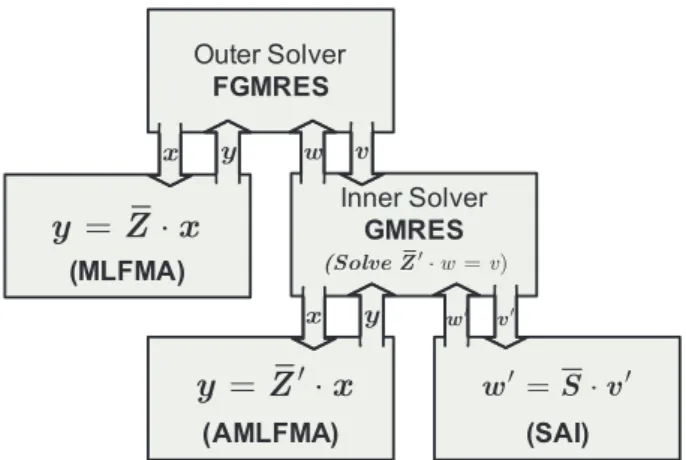
One way to make use of the far-field interactions is to embed cheaper versions of MLFMA in an inner-outer solver scheme depicted in Fig. 1 [15], [16]. The outer solver should be a flexible one to allow variations in preconditioning [4]. MLFMA with good accuracy is used here for matrix-vector multiplication. The inner solver uses a cheaper version of MLFMA, hence, compared to the near-field system, a system
that is closer to the original dense system is solved for preconditioning. The inner solver can be accelerated using an available sparse preconditioner, such as SAI.
Outer Solver FGMRES (MLFMA) Inner Solver GMRES
y
=
Z x
⋅
(AMLFMA) (SAI)y
=
Z
′
⋅
x
w′=S v⋅ ′ y x w v y x w′ v′ w v (Solve Z′ ⋅ = )Fig. 1. Inner-outer solution scheme.
Inexpensive versions of MLFMA can be obtained by relax-ing the accuracy, which can be performed in several ways. In our approach, we balance the accuracy and efficiency in a flexible way by redefining the truncation number for level l as
L0
l= L1+ af(Ll− L1), (19)
where L1 is the truncation number defined for the first level,
Llis the original truncation number for the level l calculated
by using the translation function
L ≈ 1.73ka + 2.16(d0)2/3(ka)1/3. (20)
In the above, a is the cluster size of the level and d0 is the
number of accurate digits [17]. The approximation factor af is
defined in the range from 0.0 to 1.0. As af increases from 0.0
to 1.0, the AMLFMA becomes more accurate but less efficient,
while it corresponds to the full MLFMA when af = 1. Hence,
this parameter provides us important flexibility in designing the preconditioner. Moreover, the truncation number of the lowest level is not modified, hence AMLFMA does not require extra computation load for the radiation and receiving patterns of the basis and testing functions when it is used in conjunction with MLFMA in a nested manner.
We compare the change in truncation numbers for different approaches in Fig. 2. IMLFMA represents the “incomplete MLFMA,” which is obtained by completely ignoring the interactions after the fifth level for this problem. We note that the computation time of the operations for a level is
proportional to L2[18]. Therefore, we expect significant gains
for low approximation factors, especially as the number of levels increase.
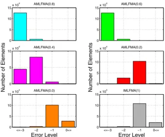
To demonstrate the accuracy of AMLFMA, we analyze the relative error in the output vector y for the matrix-vector product y = A · x, where x is a vector of ones. In Fig. 3, we show the number of elements of the output vector y satisfying different error levels. We also show radar-cross-section (RCS) results for several approximation factors and
1 2 3 4 5 6 0 20 40 60 80 100 120 Levels Truncation Number MLFMA AMLFMA(0.8) AMLFMA(0.6) AMLFMA(0.4) AMLFMA(0.2) AMLFMA(0.0) IMLFMA
Fig. 2. Comparison of truncation numbers for different approximation strategies. The geometry is a 12λ-sphere with 132,003 unknowns.
their comparisons with analytical results in Fig. 4. Since we consider the worst-case scenario for the positions of the basis and testing functions to guarantee the desired level of accuracy, we achieve moderately accurate matrix-vector multiplications with low approximation factors such as 0.2. On the other hand, these approximations do not provide accurate enough results for RCS. Hence, this strategy is useful in designing powerful preconditioners, where the accuracy is not critical.
0 5 10 15x 10 4 AMLFMA(0.8) 0 5 10 15x 10 4 AMLFMA(0.6) 0 5 10x 10 4 AMLFMA(0.4) Number of Elements 0 5 10 15x 10 4 AMLFMA(0.2) Number of Elements <=−3 −2 −1 0<= 0 5 10 15x 10 4 AMLFMA(0.0) Error Level <=−3 −2 −1 0<= 0 5 10 15x 10 4 IMLFMA(1) Error Level
Fig. 3. Error levels of AMLFMA with various values of affor a 12λ-sphere
with 132,003 unknowns. The reference is MLFMA with three accurate digits.
By analyzing the error plots in Fig. 3, we can make a good choice for the stopping criteria of the inner solver. For AMLFMA with 0.2 approximation factor, almost all elements of the output vector y are computed with less than 0.1 error with respect to full MLFMA, while the computation time is significantly reduced. Hence, if we fix the error threshold of the inner solver at 0.1, AMLFMA(0.2) seems to be the best choice. A more rigid stopping criterion would necessitate a more accurate matrix-vector multiplication, whose computa-tion time cannot be reduced so much.
We should mention that there are other studies in the context
−60 −40 −20 0 20 40 Approximation Factor: 1.0 Analytical Computational Error −60 −40 −20 0 20 40 Approximation Factor: 0.8 −60 −40 −20 0 20 40 Total RCS (dB) Approximation Factor: 0.6 −60 −40 −20 0 20 40 Total RCS (dB) Approximation Factor: 0.4 0 45 90 135 180 −60 −40 −20 0 20 40 Approximation Factor: 0.2 Bistatic Angle 0 45 90 135 180 −60 −40 −20 0 20 40 Approximation Factor: 0.0 Bistatic Angle
Fig. 4. RCS plots and their comparisons with the analytical solution for a 12λ-sphere with 132,003 unknowns.
of MLFMA that make use of both near-field and far-field information [19], [20]. In those studies, spectral information is explicitly computed via iterative eigensystem solvers and then this information is used to obtain a two-level preconditioner. Since the setup time of this preconditioner can be very high, these preconditioners suit for monostatic RCS calculations involving many RHS vectors.
C. Preconditioning EFIE Systems
In Fig. 5, we show the pseudospectra [21] of an EFIE matrix related to a problem with 930 unknowns. The matrix properties are very unfavorable for the iterative solution. The eigenvalues are scattered, especially along the left half-plane, making the matrix highly indefinite. Moreover, the 0.1-pseudospectrum includes the origin, signalling the near-singularity of the matrix. Hence preconditioning is indispensable for EFIE not only for efficiency but also for robustness.
Because of the high indefiniteness of EFIE matrices, ILU(0) is very likely to fail, though it is reported to work well for small problems [22]. The more robust preconditioner, ILUT, may also fail due to small pivots. Hence, pivoting may be necessary to increase the robustness [5].
We stress that SAI is a robust preconditioner and does not suffer from the instability problem. However, for highly
-2 -1.5 -1 -0.5 0 0.5 1 -0.2 0 0.2 0.4 0.6 0.8 1 EFIE -1.5 -1.25 -1
Fig. 5. Pseudospectrum of an EFIE matrix. The problem is a sphere with 930 unknowns.
indefinite problems, it is shown that SAI is not as effective as ILU-type preconditioners [23]. To provide a better
ap-proximation to the ZNF, we solve the near-field system in
an inner-outer solution scheme. We use SAI for the iterative solution of the near-field system and then the original system is preconditioned by this near-field solution. This scheme, which we call the iterative near-field preconditioner, yields a forward-type preconditioner, similar to ILU. The difference is that, in ILU, the preconditioner that approximates the near-field matrix is already in factorized form and for a given RHS vector y, the system (11) is solved by using backward and forward solves. On the other hand, for the preconditioning scheme described, the preconditioner is the exact near-field matrix, i.e.,
M = ZN F, but we approximately solve the system (11) by an iterative method. Here, again, the preconditioning operation changes from iteration to iteration, hence a flexible Krylov method should be used. The effectiveness of SAI is further improved with this scheme for EFIE systems [24], [25].
For very large problems with millions of unknowns, the near-field itself becomes a crude approximation to the dense system matrix. Hence, it is not unlikely that neither SAI, nor the iterative near-field preconditioner succeed to converge iterative solvers. Hence, it is obligatory to use preconditioners that make use of far-field elements, such as AMLFMA.
D. Preconditioning CFIE Systems
The pseudospectra of a CFIE matrix is shown in Fig. 6. In contrast to EFIE, the eigenvalues of the CFIE matrix are fairly clustered and they are closer to the right half-plane. Moreover, the CFIE matrix is closer to being normal, which is advantageous for non-symmetric solvers such as GMRES.
-2 -1.5 -1 -0.5 0 0.5 1 -0.2 0 0.2 0.4 0.6 0.8 1 CFIE -1.5 -1.25 -1
Fig. 6. Pseudospectrum of a CFIE matrix. The problem is a sphere with 930 unknowns.
Considering these favorable properties, it is not difficult to foresee that ILU(0) works well for CFIE matrices. For parallel applications, a SAI preconditioner that uses the same nonzero
pattern of ZNF works well for large problems. However, it
may be advantageous to use stronger AMLFMA precondi-tioner that makes use of the far-field elements for efficiency.
IV. RESULTS
In this section, we demonstrate the performance of the aforementioned preconditioners on integral-equation formu-lations. Among the problems considered here, the square patch (P) and the half sphere (HS) have open surfaces. Therefore, they are inevitably modelled by EFIE. The closed targets Flamme (F), which is a stealth geometry [26], and the helicopter (H) are modelled by CFIE. These open-surface and closed-surface problems are illustrated in Figs. 7 and 8, respectively. PATCH (P)
x
y
z
L = 0.3mFig. 7. Open geometries used in the numerical experiments.
Fig. 8. Closed geometries used in the numerical experiments.
In our experiments, we use the GMRES solver for its robustness. We try to reduce the norm of the initial residual
by 10−6 in a maximum of 1,000 iterations, unless stated
otherwise.
A. Solution of Open Problems via EFIE
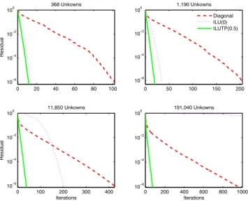
As discussed in Section III-C, ILU(0) is not expected to succeed in EFIE problems. We confirm this in Figs. 9 and 10, where we present the residual plots for the patch and the half sphere with increasing number of unknowns. For the patch, since pivoting does not change the results, we provide only the ILUT results. From the figures we see that, due to unfavorable spectral properties of EFIE matrices, even robust iterative solvers such as the no-restart GMRES, cannot succeed with
simple preconditioners, such as the diagonal preconditioner. Regarding the ILU-type preconditioners, it is evident that as
the number of unknowns increases and ZNFbecomes sparser,
ILU(0) becomes useless. Sometimes ILUT or ILUTP with 1.0 pivoting fails as in the half-sphere case. On the other hand, we find ILUT with 0.5 pivoting tolerance (ILUTP(0.5)) very successful on all EFIE problems.
In Table I, we show the condest values and iteration counts for the patch and the half sphere. From the large condest values of Table I, we understand that the failure of ILU(0) and ILUT (for the half sphere) is because of the instable factors. For ILUTP(0.5), condest values are low and we have convergence in reasonable numbers of iterations.
0 20 40 60 80 100 10−6 10−4 10−2 100 368 Unkowns Residual 0 50 100 150 200 10−6 10−4 10−2 100 1,190 Unkowns Diagonal ILU(0) ILUTP(0.5) 0 100 200 300 400 10−6 10−4 10−2 100 11,850 Unkowns Iterations Residual 0 200 400 600 800 1000 10−6 10−4 10−2 100 191,040 Unkowns Iterations
Fig. 9. Plots of residual versus iterations for diagonal and ILU-type preconditioners. The target object is a patch.
0 50 100 150 200 250 10−6 10−4 10−2 100 1,564 Unkowns Residual 0 100 200 300 400 10−6 10−4 10−2 100 6,320 Unkowns Diagonal ILU(0) ILUT ILUTP(0.5) 0 200 400 600 10−6 10−4 10−2 100 25,408 Unkowns Iterations Residual 0 200 400 600 800 1000 10−6 10−4 10−2 100 101,888 Unkowns Iterations
Fig. 10. Plots of residual versus iterations for diagonal and ILU-type preconditioners. The target object is a half sphere.
For parallel implementations, we first compare SAI and NF/SAI preconditioners on larger problems in Table II. We
TABLE I
NUMBER OF ITERATIONS ANDcondestVALUES FORILU-TYPE PRECONDITIONERS
Geo- ILU(0) ILUT ILUTP(0.5)
metry N condest Iter condest Iter condest Iter
P1 368 40 9 40 7 39 7 P2 1,190 117 27 56 12 57 11 P3 11,850 5,015 202 375 28 307 23 P4 191,040 2.E+07 - 4,559 49 755 46 HS1 383 36 24 32 19 29 17 HS2 914 154 49 67 33 56 26 HS3 25,408 8,670 620 2.E+06 758 220 67 HS4 239,624 7.E+06 - 1.E+11 - 894 150
Note: “-” indicates that convergence is not attained in 1,000 iterations. TABLE II
PERFORMANCE COMPARISON OFSAIANDNF/SAIPRECONDITIONERS
Geo- NF-LU SAI INF
metry N Iter Iter Time (s) Iter Time (s)
P1 12,249 26 44 12 29 9 P2 137,792 53 91 336 59 253 P3 3,164,544 - 253 7,621 165 5,387 HS1 9,911 38 60 24 40 17 HS2 116,596 93 156 510 103 383 HS3 2,554,736 - 547 17,404 380 12,286
Note: “-” indicates that the solution cannot be obtained since the memory limitation is exceeded.
TABLE III
PERFORMANCE COMPARISON OFSAIANDAMLFMAPRECONDITIONERS
SAI AMLFMA
Geo- Iter
metry N Iter Time (s) Outer Inner Time (s)
P1 197,424 89 104 15 141 67 P2 790,656 128 654 23 222 388 P3 3,164,544 195 5,679 36 354 2,740 P4 12,662,016 275 33,557 53 526 16,184 P5 21,965,824 - - 9 85 24,689 HS1 159,452 174 306 24 238 168 HS2 638,392 321 2,243 44 439 1,076 HS3 2,554,736 547 17,352 70 700 6,634 HS4 10,221,280 - - 44 440 20,774
Note: “-” indicates that the solution cannot be obtained due to memory limitations. P5 and HS4 is solved with 10−3stopping tolerance.
also give the number of iterations for the exact solution of the near-field system (NF-LU) for benchmarking. For SAI, we use the same sparsity pattern as the original system. For the iterative near-field preconditioner (INF), the stopping criteria of the inner solver is set to one order residual drop or a maximum of five iterations. The results presented in Table II reveal that such a crude solution of the near-field system outperforms SAI and produces iteration counts that are very close to those of NF-LU. The solution times are also significantly reduced compared to SAI.
Then, we compare SAI to the AMLFMA preconditioner in Table III. The large problems P4 and HS3 that are solvable with SAI can be solved two times and three times faster, re-spectively, with the AMLFMA preconditioner. This is because of the insufficiency of the near-field matrix for large systems,
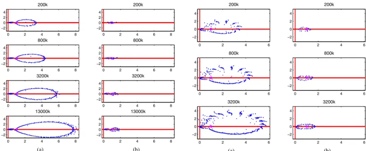
0 2 4 6 8 −2 0 2 4 200k 0 2 4 6 8 −2 0 2 4 200k 0 2 4 6 8 −2 0 2 4 800k 0 2 4 6 8 −2 0 2 4 800k 0 2 4 6 8 −2 0 2 4 3200k 0 2 4 6 8 −2 0 2 4 3200k 0 2 4 6 8 −2 0 2 4 13000k 0 2 4 6 8 −2 0 2 4 13000k (a) (b)
Fig. 11. Approximate eigenvalues computed by the GMRES solver for the patch problem employing (a) SAI and (b) AMLFMA preconditioners.
−0.2 −0.1 0 0.1 0.2 −0.2 0 0.2 200k −0.2 −0.1 0 0.1 0.2 −0.2 0 0.2 200k −0.2 −0.1 0 0.1 0.2 −0.2 0 0.2 800k −0.2 −0.1 0 0.1 0.2 −0.2 0 0.2 800k −0.2 −0.1 0 0.1 0.2 −0.2 0 0.2 3200k −0.2 −0.1 0 0.1 0.2 −0.2 0 0.2 3200k −0.2 −0.1 0 0.1 0.2 −0.2 0 0.2 13000k −0.2 −0.1 0 0.1 0.2 −0.2 0 0.2 13000k (a) (b)
Fig. 12. Approximate eigenvalues near the origin computed by the GMRES solver for the patch problem employing (a) SAI and (b) AMLFMA precon-ditioners.
as discussed in Section III-B. For the largest problems H5 and S4, the SAI preconditioner requires too many iterations. H5 and S4 could not be solved with the no-restart GMRES, which stores the previous Krylov vectors to generate next iterate. Hence, these problems can only be solved with AMLFMA, since it requires fewer iterations. We emphasize that the largest patch problem involves approximately 22 million unknowns and it is the largest problem solved with EFIE, to the best of our knowledge.
To provide more insight to the SAI and AMLFMA pre-conditioners, Figs. 11–14 present approximate eigenvalues computed by the GMRES solver as a by-product. These are actually the eigenvalues of the Hessenberg matrix, which is
0 2 4 6 −2 0 2 4 200k 0 2 4 6 −2 0 2 4 200k 0 2 4 6 −2 0 2 4 800k 0 2 4 6 −2 0 2 4 800k 0 2 4 6 −2 0 2 4 3200k 0 2 4 6 −2 0 2 4 3200k (a) (b)
Fig. 13. Approximate eigenvalues computed by the GMRES solver for the half-sphere problem employing (a) SAI and (b) AMLFMA preconditioners.
−0.2 −0.1 0 0.1 0.2 −0.2 −0.1 0 0.1 0.2 200k −0.2 −0.1 0 0.1 0.2 −0.2 −0.1 0 0.1 0.2 200k −0.2 −0.1 0 0.1 0.2 −0.2 −0.1 0 0.1 0.2 800k −0.2 −0.1 0 0.1 0.2 −0.2 −0.1 0 0.1 0.2 800k −0.2 −0.1 0 0.1 0.2 −0.2 −0.1 0 0.1 0.2 3200k −0.2 −0.1 0 0.1 0.2 −0.2 −0.1 0 0.1 0.2 3200k (a) (b)
Fig. 14. Approximate eigenvalues near the origin computed by the GMRES solver for the half-sphere problem employing (a) SAI and (b) AMLFMA preconditioners.
the projection of the system matrix onto the Krylov subspace. These eigenvalues are known to approximate well the bound-ary of the spectra [2], hence providing useful information regarding the convergence of iterative solutions. From Figs. 11 and 13, we see that AMLFMA is more successful than SAI in clustering the eigenvalues. Moreover, the zoomed plots in Figs. 12 and 14 indicate that SAI leaves many eigenvalues close to zero, hence requiring high numbers of iterations for convergence.
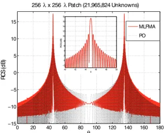
To verify the accuracy of the largest patch problem, we compare the MLFMA solution with a physical-optics (PO) solution in Fig. 15. The incoming field is a y-oriented plane
0 20 40 60 80 100 120 140 160 180 −15 −10 −5 0 5 10 15 θ 256 λx 256 λ Patch (21,965,824 Unknowns) RCS (dB) MLFMA PO 40 42 44 46 48 50 −2 0 2 4 6 8 10 12 14 16 18 θ RCS (dB)
Fig. 15. Comparison the MLFMA solution with the PO solution for the 256λ patch.
this is a 256λ patch, we expect the PO solution to be accurate
for the specular reflection (θ = 45◦, φ = 180◦) and forward
scattering (θ = 135◦, φ = 180◦). Hence, the accuracy of the
MLFMA solution is verified with a good agreement between the two methods at these points.
B. Solution of Closed Problems via CFIE
Due to the better conditioning of CFIE, ILU(0) is expected to be free from instability problems. In fact, the condest values and the iteration counts turn out to be very similar for all ILU-type preconditioners [12]. Therefore, we prefer to use ILU(0), which has a very low setup time.
In Fig. 16, we compare ILU(0) to the block-diagonal and SAI preconditioners. ILU(0) performs remarkably better com-pared to the block-diagonal preconditioner. The total solution time is halved for Flamme, and is reduced by 75% for the helicopter. Even though SAI has iteration numbers close to those of ILU(0), the setup time of SAI is much larger than ILU(0). Hence, the total solution time of SAI exceeds those of the other two preconditioners.
Flamme Helicopter 0 10 20 30 40 50 60 70
Total Time (minutes)
SAI
Block−Diagonal ILU(0)
Fig. 16. Total sequential solution times (setup + iterations) for Flamme with 197,892 unknowns and helicopter with 185,532 unknowns.
Flamme Helicopter 0 50 100 150 200
Total Time (minutes) Block−Diagonal
SAI AMLFMA
Fig. 17. Total parallel solution times (setup + iterations) for Flamme with 3,581,628 unknowns and helicopter with 2,957,616 unknowns.
For parallel implementations, the block-diagonal precondi-tioner is commonly used for CFIE, because of its ease of parallelization and the low setup time. On the other hand, particularly for complex targets, such as Flamme and heli-copter, we observe that the solution times can be significantly improved by using a better preconditioner, such as SAI or the AMLFMA preconditioner. We support this claim by compar-ing the solution of large closed-surface problems in Fig. 17. For Flamme, even though the iteration counts of SAI are much smaller than those of the block-diagonal preconditioner, because of the larger setup time of SAI, there is not a significant difference between the total solution times of these preconditioners. However, for helicopter the gain is around 40% with SAI. Furthermore, for bistatic RCS calculations, the gains can be much higher.
On the other hand, the AMLFMA preconditioner performs outstandingly better with respect to the block-diagonal precon-ditioner. The solution times are reduced by 35% for Flamme and 75% for the helicopter. Hence, for large-scale problems, it is wise to construct preconditioners that make use of more than the sparse near-field matrix in an efficient manner.
V. CONCLUSIONS
In this paper, we evaluate several preconditioners for integral-equation problems. We consider both the EFIE for-mulation that is essential for open geometries and the better-conditioned CFIE formulation that is applicable to both open and closed geometries.
The EFIE formulation yields highly indefinite matrices, for which preconditioning is crucial for the convergence of iterative methods. Even though the CFIE matrices are better conditioned, rapid solution of large real-life problems neces-sitates preconditioning.
Our experiments with the sequential programs reveal that ILU preconditioners can be safely applied to integral-equation methods, provided that pivoting is applied to ILUT for EFIE systems. For CFIE, ILU(0) is a very strong alternative to the block-diagonal preconditioner. ILU-type preconditioners are the most widely used and established methods in numerical analysis, and they are available in solver packages, such as
PETSc [10]. Hence, we strongly recommend their use for sequential problems.
For larger problems, on the other hand, one should resort to SAI preconditioners, which can be efficiently parallelized. Up to certain sizes, SAI enables fast convergence for both CFIE and EFIE. For EFIE, SAI can be made even stronger by embedding it in an inner-outer solution scheme that uses the iterative solution of the near-field system for preconditioning. On the other hand, for very large problems, the near-field system does not provide a good approximation to the dense system matrix. Therefore, preconditioners that are built from the near-field interactions cannot be effective. Considering this fact, we develop the AMLFMA preconditioner. Taking into account the far-field interactions as well as near-field interactions, AMLFMA preconditioner succeeds to solve ultra large EFIE and CFIE systems in reasonable solution times. In particular, we are able to solve a patch problem involving approximately 22 million unknowns in less than seven hours. We verify the accuracy of the solution by comparing the problem with a PO solution. To the best of our knowledge, this is the solution of the largest EFIE problem ever reported.
ACKNOWLEDGMENT
This work was supported by the Scientific and Technical Research Council of Turkey (TUBITAK) under Research Grant 105E172, by the Turkish Academy of Sciences in the framework of the Young Scientist Award Program (LG/TUBA-GEBIP/2002-1-12), and by contracts from ASELSAN and SSM. Computer time was provided in part by a generous allocation from Intel Corporation.
REFERENCES
[1] W. C. Chew, J.-M. Jin, E. Michielssen, and J. Song, Eds., Fast and Efficient Algorithms in Computational Electromagnetics. Norwood, Ma, Usa: Artech House, Inc., 2001.
[2] L. N. Trefethen and David Bau, III, Numerical Linear Algebra. Philadelphia, USA: SIAM, 1997.
[3] M. Benzi, “Preconditioning techniques for large linear systems: a survey,” J. Comput. Phys., vol. 182, no. 2, pp. 418–477, 2002. [4] Y. Saad, Iterative Methods for Sparse Linear Systems, 2nd ed.
Philadel-phia, USA: SIAM, 2003.
[5] E. Chow and Y. Saad, “Experimental study of ILU preconditioners for indefinite matrices,” J. Comput. Appl. Math., vol. 86, no. 2, pp. 387–414, 1997.
[6] E. Chow, “A priori sparsity patterns for parallel sparse approximate inverse preconditioners,” SIAM J. Sci. Comput., vol. 21, no. 5, pp. 1804– 1822, 2000.
[7] M. J. Grote and T. Huckle, “Parallel preconditioning with sparse approximate inverses,” SIAM J. Sci. Comput., vol. 18, no. 3, pp. 838– 853, 1997.
[8] E. Chow, “Parallel implementation and practical use of sparse approxi-mate inverse preconditioners with a priori sparsity patterns,” Int. J. High Perform. Comput. Appl., vol. 15, no. 1, pp. 56–74, 2001.
[9] K. Chen, Matrix Preconditioning Techniques and Applications, 2nd ed., ser. Cambridge Monographs on Applied and Computational Mathemat-ics. Cambridge, UK: Cambridge University Press, 2005, vol. 19. [10] S. Balay, W. D. Gropp, L. C. McInnes, and B. F. Smith, “PETSc
users manual,” Argonne National Laboratory, Tech. Rep. ANL-95/11 - Revision 2.1.5, 2004.
[11] M. Bollh¨ofer and Y. Saad, “ILUPACK - preconditioning software pack-age,” 2004, available online at http://www.math.tu-berlin.de/ilupack/.
[12] T. Malas and L. G¨urel, “Incomplete LU preconditioning with the multilevel fast multipole algorithm for electromagnetic scattering,” SIAM J. Sci. Comput., vol. 29, no. 4, pp. 1476–1494, 2007, DOI: 10.1137/060659107.
[13] J. Lee, J. Zhang, and C.-C. Lu, “Incomplete LU preconditioning for large scale dense complex linear systems from electromagnetic wave scattering problems,” J. Comput. Phys., vol. 185, no. 1, pp. 158–175, 2003.
[14] ——, “Sparse inverse preconditioning of multilevel fast multipole al-gorithm for hybrid integral equations in electromagnetics,” IEEE Trans. Antennas and Propagation, vol. 52, no. 9, pp. 158–175, 2004. [15] B. Carpentieri, I. S. Duff, L. Giraud, and G. Sylvand, “Combining fast
multipole techniques and an approximate inverse preconditioner for large electromagnetism calculations,” SIAM J. Sci. Comput., vol. 27, no. 3, pp. 774–792, 2005.
[16] V. Simoncini and D. B. Szyld, “Flexible inner-outer krylov subspace methods,” SIAM J. Numer. Anal., vol. 40, no. 6, pp. 2219–2239, 2002. [17] M. L. Hastriter, S. Ohnuki, and W. C. Chew, “Error control of the translation operator in 3D MLFMA,” Microwave Opt. Technol. Lett., vol. 37, no. 3, pp. 184–188, 2003.
[18] ¨O. S. Erg¨ul, “Fast multipole method for the solution of electromag-netic scattering problems,” Master’s thesis, Bilkent University, Ankara, Turkey, 2003.
[19] I. S. Duff, L. Giraud, J. Langou, and E. Martin, “Using spectral low rank preconditioners for large electromagnetic calculations,” CERFACS, Toulouse, France, Technical Report TR/PA/03/95, 2003, preliminary version of the article published in IJNME, vol. 62, nber 3, pp 416-434. [20] P.-L. Rui, R.-S. Chen, D.-X. Wang, and E. K.-N. Yung, “Spectral two-step preconditioning of multilevel fast multipole algorithm for the fast monostatic RCS calculation,” IEEE Trans. Antennas Propogat., vol. 55, no. 8, pp. 2268–2275, Aug. 2007.
[21] L. N. Trefethen, “Computation of pseudospectra,” Acta Numerica, vol. 8, no. 1, pp. 247–295, 1999.
[22] K. Sertel and J. L. Volakis, “Incomplete LU preconditioner for FMM implementation,” Microw. Opt. Tech. Lett., vol. 28, pp. 265–267, 2000. [23] M. Benzi and M. Tuma, “A comparative study of sparse approximate inverse preconditioners,” Applied Numerical Mathematics: Transactions of IMACS, vol. 30, no. 2–3, pp. 305–340, 1999.
[24] T. Malas and L. G¨urel, “Strengthening near-field preconditioners using flexible solvers,” Bilkent University, Tech. Rep., 2006.
[25] Z. H. Fan, R. S. Chen, E. K. N. Yung, and D. X. Wang, “Inner-outer GMRES algorithm for MLFMA implementation,” in IEEE Antennas and Propagation Society International Symposium, 2005, pp. 463–466. [26] L. G¨urel, H. Ba˜gcı, J.-C. Castelli, A. Cheraly, and F. Tardivel,
“Valida-tion through comparison: Measurement and calcula“Valida-tion of the bistatic radar cross section of a stealth target,” Radio Science, vol. 38, no. 3, pp. 1046–1058, 2003.