A HYBRID HAIR MODEL USING THREE
DIMENSIONAL FUZZY TEXTURES
a thesis
submitted to the department of computer engineering
and the institute of engineering and science
of bilkent university
in partial fulfillment of the requirements
for the degree of
master of science
By
Medeni Erol Aran
January, 2007
I certify that I have read this thesis and that in my opinion it is fully adequate, in scope and in quality, as a thesis for the degree of Master of Science.
Assoc. Prof. Dr. U˘gur G¨ud¨ukbay (Advisor)
I certify that I have read this thesis and that in my opinion it is fully adequate, in scope and in quality, as a thesis for the degree of Master of Science.
Prof. Dr. Enis C¸ etin
I certify that I have read this thesis and that in my opinion it is fully adequate, in scope and in quality, as a thesis for the degree of Master of Science.
Asst. Prof. Dr. Tolga C¸ apın
Approved for the Institute of Engineering and Science:
Prof. Dr. Mehmet B.Baray Director of the Institute
ABSTRACT
A HYBRID HAIR MODEL USING THREE
DIMENSIONAL FUZZY TEXTURES
Medeni Erol Aran M.S. in Computer Engineering
Supervisor: Assoc. Prof. Dr. U˘gur G¨ud¨ukbay January, 2007
Human hair modeling and rendering have always been a challenging topic in computer graphics. The techniques for human hair modeling consist of explicit geometric models as well as volume density models. Recently, hybrid cluster models have also been successful in this subject. In this study, we present a novel three dimensional texture model called 3D Fuzzy Textures and algorithms to generate them. Then, we use the developed model along with a cluster model to give human hair complex hairstyles such as curly and wavy styles. Our model requires little user effort to model curly and wavy hair styles. With this study, we aim at eliminating the drawbacks of the volume density model and the cluster hair model with 3D fuzzy textures. A three dimensional cylindrical texture map-ping function is introduced for mapmap-ping purposes. Current generation graphics hardware is utilized in the design of rendering system enabling high performance rendering.
Keywords: Hair modeling, hair rendering, curly hair, wavy hair, cluster hair model, volume density model, 3D texture, 3D texture mapping.
¨
OZET
¨
UC
¸ BOYUTLU BULANIK DOKULAR KULLANAN
KARMA SAC
¸ MODEL˙I
Medeni Erol Aran
Bilgisayar M¨uhendisli˘gi, Y¨uksek Lisans Tez Y¨oneticisi: Do¸c. Dr. U˘gur G¨ud¨ukbay
Ocak, 2007
˙Insan sa¸cının modellenmesi ve ı¸sıklandırılması bilgisayar grafi˘gi alanında daima ilgi ¸ceken konulardan biri olmu¸stur. A¸cık geometrik modeller ve kapalı hacim yo˘gunlu˘gu modelleri, insan sa¸cının modellenmesi ve ı¸sıklandırılması i¸cin geli¸stirilen tekniklerdendir. Bu tekniklerle birlikte, karma tutam modelleri de son zamanlarda bu konuda ba¸sarılı olmu¸stur. Bu ¸calı¸smada, 3 Boyutlu Karma¸sık Dokular ismini verdi˘gimiz yeni bir ¨u¸c boyutlu doku modeli ve bunun ¨uretilmesi anlatılmaktadır. Daha sonra, bu doku modeli kullanılarak kıvırcık ve dalgalı sa¸c modeli gibi karma¸sık sa¸c ¸sekilleri karma tutam modeliyle birle¸stirilerek kul-lanılmaktadır. Geli¸stirdi˘gimiz model, kıvırcık ve dalgalı sa¸c modelleme i¸cin gereken kullanıcı eforunu azaltmaktadır. Bu ¸calı¸sma ile, hacim yo˘gunlu˘gu mod-elinin ve karma tutam modmod-elinin yetersizliklerini gidermeyi hedeflemekteyiz. Dokuların ¨ort¨u¸st¨ur¨ulmesi amacıyla ¨u¸c boyutlu bir silindirik doku ¨ort¨u¸st¨urme fonksiyonu sunulmaktadır. I¸sıklandırma sisteminin tasarımında, yeni nesil ekran kartlarının sa˘gladı˘gı imkanlardan yararlanılarak y¨uksek performanslı ı¸sıklandırma sa˘glanmı¸stır.
Anahtar s¨ozc¨ukler: Sa¸c modelleme, sa¸c ı¸sıklandırma, kıvırcık sa¸c, dalgalı sa¸c, karma tutam sa¸c modeli, hacim yo˘gunlu˘gu sa¸c modeli, ¨u¸c boyutlu doku, ¨u¸c boyutlu doku ¨ort¨u¸st¨urme.
Acknowledgement
I gratefully thank to my supervisor Assoc. Prof. Dr. U˘gur G¨ud¨ukbay for his instructive comments and endless support in the supervision of the thesis.
I am gratefully thankful to Prof. Dr. B¨ulent ¨Ozg¨u¸c for introducing me the fundamental concepts on fur and hair modeling and reviewing the thesis.
I would also like to give special thanks to my thesis committee members Prof. Dr. Enis C¸ etin and Asst. Prof. Dr. Tolga C¸ apın for their valuable comments.
Besides, I would like to thank Yusuf Bediz for his invaluable support.
Finally, I would like to express my deepest thanks to my father and mother for making it possible.
Contents
1 Introduction 1
1.1 Motivation . . . 2
1.2 Organization of the Thesis . . . 3
2 Related Work 4 2.1 Explicit Geometric Models . . . 4
2.2 Volume Density Models . . . 5
2.3 Cluster Models . . . 6
3 3D Fuzzy Textures 8 3.1 The Texels Approach . . . 8
3.2 Splines as Hair Strands . . . 9
3.2.1 Parametric Curves . . . 9
3.3 Growing Hairs within 3D Textures . . . 13
3.3.1 Seed Hairs for the Unit Cube . . . 14
3.4 From Cardinal Splines to Texels . . . 17
CONTENTS vii
3.4.1 Intersecting Cardinal Splines with Texels . . . 18
3.4.2 Marching Cells . . . 19
3.4.3 Antialiasing during Texel Conversion . . . 19
4 Limitations of Single Level Abstraction 23 4.1 Cloth Simulation for 3D Texture Mapping . . . 23
5 Second Level of Abstraction 28 5.1 The Cluster Hair Model . . . 28
5.2 Generalized Cylinders . . . 29
5.3 Generalized Cylinders as Hair Clusters . . . 31
5.4 Slicing of Generalized Cylinders . . . 33
5.5 Global Hair Cluster Placement . . . 34
5.6 Mapping of Fuzzy Textures onto Slices . . . 36
6 Rendering 38 6.1 System Overview . . . 38 6.1.1 Hair Renderer . . . 39 6.1.2 Non-Hair Renderer . . . 43 6.1.3 Image Compositor . . . 43 6.2 Shading . . . 44 7 Experimental Results 46
CONTENTS viii
7.1 Visual Results For 3D Fuzzy Textures . . . 46
7.2 Visual Results for Single Level Abstraction with Fuzzy Textures . 49
7.3 Visual Results for Two Level Abstraction with Fuzzy Textures . . 50
7.4 Performance Considerations . . . 53
7.5 Implementation Details . . . 55
List of Figures
2.1 Shells and fins approach (adopted from [15]) . . . 7
3.1 A cubic spline generated from eight control points . . . 11
3.2 A cardinal spline segment . . . 12
3.3 Effect of tension parameter for a Cardinal spline . . . 14
3.4 Some seed strands for the unit cube . . . 14
3.5 Sample hair root placements for different Poisson distance con-straints: (a) d = 0.02; and (b) d = 0.07. . . 16
3.6 Self similar clusters of seed hairs . . . 17
3.7 Marching cells algorithm. (a)Marching starts at strand root; (b)texel conversion for two cells; (c) conversion is getting closer to end; and (d) completed conversion. . . 21
4.1 A triangular mesh head model . . . 24
4.2 A rectangular grid over the model . . . 25
4.3 Simulation of cloth over the head model: (a) A frame from the simulation study; (b) steady state. . . 25
LIST OF FIGURES x
4.4 A closer look of the steady state at the top of the target surface . 26
4.5 A short punky hair style . . . 26
5.1 A generalized cylinder with some of its contours (reprinted from [4]) 32 5.2 A generalized cylinder . . . 33
5.3 Slicing between the contours of a generalized cylinder . . . 35
5.4 An example global cluster placement . . . 35
5.5 Mapping of a 3D texture onto a generalized cylinder . . . 37
6.1 The framework of the rendering system . . . 40
6.2 The framework for the slice rendering process . . . 41
6.3 Meta textures rendering process model . . . 42
6.4 Non-hair rendering process model . . . 43
6.5 Image composition process model . . . 44
7.1 3D texture with straight texels . . . 47
7.2 A 3D fuzzy texture without clustering in the unit cube . . . 47
7.3 A 3D fuzzy texture with clustering in the unit cube . . . 48
7.4 Multiple 3D fuzzy textures . . . 48
7.5 Single level abstraction with 3D fuzzy textures . . . 49
7.6 Generalized cylinder mapped with a 3D fuzzy texture . . . 51
LIST OF FIGURES xi
7.8 A head model with fine detailed hair grown with fuzzy textures . 52
7.9 A front facing head model with long wavy hair . . . 52
Chapter 1
Introduction
In the last decade, there have been great achievements in the area of computer graphics. These achievements appear in our everyday lives. Films full of visual effects and computer games with natural looking artificial scenes enrich our lives. Besides, scientific visualization provides very valuable information for physicians to save people’s lives.
Modeling and visualization of complex data has always been a very challenging problem in computer graphics. Human hair is one of such examples and there has been significant progress in modeling realistic human hair in the last decade [12, 24, 15, 17]. However, there are some unresolved issues in this subject. For example, modeling curly and wavy hair styles are still very difficult and time consuming with classical techniques.
The main difficulty of hair modeling is the fact that hair may be in very differ-ent styles. Besides, there are a lot of hair strands in sub pixel size even within a small volume of hair group. Optic characteristics of hair are also complex. Since hair is transparent and there are so many of them in a small volume, interaction of these transparent strands with light results in an extraordinary bidirectional reflection distribution function (BRDF). Dynamic simulation is also problematic because of physical interaction of huge number of hair strands. Realistic hu-man hair representation contains problems in all aspects of computer graphics
CHAPTER 1. INTRODUCTION 2
technologies, i.e. shape modeling, rendering and animation.
During nearly the thirty years of study, several methods have been developed for generating hair. From early times of fur modeling and rendering until now, re-searchers generated breathtaking images of human hair using different techniques. However, most of these methods are applicable only to particular types of hair under specific conditions. Curly and wavy hairstyles have always been problem-atic in hair modeling since it requires a lot of user interaction when styling the hair. Some procedural methods have also been developed. However, it is usually difficult to estimate the resulting hairstyle by using these procedural techniques. To get realistic results, one has to consider creating randomness for hair as well as preserving the main sketches of the hairstyle.
1.1
Motivation
In this study, we develop a new hair model especially for wavy and curly hair and propose a rendering architecture for the developed model. Our proposal is a hybrid model based on cluster hair model and volume density model. This study also shows the limitations of both models and discusses new techniques to eliminate the observed problems.
Our new model aims at providing the fine details of hair in a generalized 3D texture (texels) at first level of abstraction. As a second level of abstraction, these texels are mapped onto generalized cylinders that are used as global shape definers.
We develop an algorithm for creating texels from cardinal splines. Curliness of hair can easily be obtained by using these cardinal splines for fine detail. To give hair a realistic appearance we construct self similar clusters in the generalized 3D texture. Then, the conversion of geometry information to density information is performed with our curve following algorithm we developed for following a cardinal spline through a 3D texture.
CHAPTER 1. INTRODUCTION 3
Global shape definition for second level of abstraction is performed with gen-eralized cylinders. We again use cardinal splines for trajectories of gengen-eralized cylinders. Circles and ellipses are used as cross sections. Generation of 3D texture coordinates and mapping of fine detailed 3D texture for generalized cylinders is performed with a mapping function that we propose.
This study also proposes a rendering architecture for the developed model. Although ray casting gives very satisfactory visual results, it is almost impossible to get a render shot without waiting for hours. Therefore, we approximate the vol-ume characteristics of hair with polygonal slices through the generalized cylinder and use the power of conventional scan line hardware. We design and implement a generic dynamic pixel buffering algorithm [28] for Graphical Processing Units (GPU).
Shading is performed in the GPU using Kajiya and Kay’s illumination model [12] for thin cylinders. We implement image composition techniques from film industry to get final renderings in the GPU.
1.2
Organization of the Thesis
The thesis is organized as follows: Chapter 2 reviews existing hair modeling techniques in the literature. In Chapter 3, we introduce our 3D fuzzy texture model as the first level of abstraction. Chapter 4 presents the limitations of 3D textures when they are used directly as rendering primitives and offers some impermanent solutions for these limitations. Chapter 5 focuses on the second level of abstraction with generalized cylinders and our 3D texture mapping function for a permanent mapping solution. In Chapter 6, rendering architecture we propose is discussed. Chapter 7 gives the experimental results of our study. Chapter 8 presents conclusions and future research areas. Finally, Appendix gives the implementation details of the study.
Chapter 2
Related Work
The research results in modeling human hair could simply be divided into three main categories: explicit geometric models, volume density (implicit) models and cluster models. In this chapter, these approaches will be described with their advantages and disadvantages.
2.1
Explicit Geometric Models
Explicit hair models are brute force methods that try to model the geometry of each individual strand of hair using lines, curves, cylinders or surfaces. Csuri et al. [6] was the first in trying to render tribbles using triangular primitives to our knowledge. In their system, a group of tribbles were rendered with 500,000 triangles. Gavin Miller [19] stated a model by representing the individual hair strands as three forward-facing triangles arranged in the form of a cone. Although his paper was on the dynamics of snakes and worms, rendering part of his work for an artic caterpillar by such a method was also recognized by the academy. Both of these models’ problems were that they suffered from high aliasing artifacts and they were applicable only for short, straight, thick fur. Aliasing artifacts and modeling difficulty for long hair have always been an open problem for this method and there has been a great effort to eliminate these problems until today.
CHAPTER 2. RELATED WORK 5
Le Blanc et al. [13] tried to model long hair with curved cylinders.
Hadap and Thalmann used a flow-based technique for hair shape modeling [9, 10]. In their work, the hair shape is modeled as streamlines of a fluid flow. Then, the streamlines are rendered as hair strands.
In explicit models, each of the hair strands has to be defined and stored in-dividually. This was a big problem when computers had very limited memory. However, advances in computer hardware have directed researchers to focus on other problems related with this model. Aliasing is such a problem. Area antial-ising was used first to overcome this problem. Supersampling would also be used to antialias the scenes. However, even with today’s computers, rendering huge number of primitives by explicit models with oversampling is not bearable. High computational cost is another drawback of this method for the same reason.
2.2
Volume Density Models
Volume density models appeared from the fact that high complexity scenes behave more like volumetric textures. Kajiya and Kay [12] were the ones to create the state-of-the-art image known as the Teddy bear of computer graphics on fur rendering. They realized that modeling natural phenomena through density volumes created the painter’s illusion and that would be suitable for sub pixel size renderings. Meanwhile, Perlin and Hoffert [24] invented the Hypertexture and obtained very successful renderings with their method.
Kajiya and Kay named their generalized 3D volume densities as texels and used it for rendering straight fur on the Teddy bear. On the other side, hy-pertexture had the capability to model wavy fur through turbulence functions. However, both of the methods suffered from the same restriction that they were not directly suitable for modeling complex hairstyles, especially the long ones. Other restriction with those approaches was the high rendering times resulting from the volume rendering approaches used with these methods. Both the texel approach and the hypertexture approach created the state-of-the-art images on
CHAPTER 2. RELATED WORK 6
fur rendering. However, as Kajiya and Kay stated, conversion of geometry data to density data was a big problem which resulted in only straight fur with the texels approach. Also, using bilinear patches as fur containing volumes resulted in mapping problems with triangular meshes and required intensive artist effort for proper mapping.
Fabrice Neyret [21] proposed a general solution for converting geometry data to density data. In his doctorate research, he extended the texel idea for arbitrary patterns and successfully prefiltered these patterns for multiresolution texels.
2.3
Cluster Models
Cluster models aim to use the powerful sides of both explicit methods and im-plicit methods. Exim-plicit methods have the advantage of using hardware support. However, direct rendering through geometry does not produce qualified images. On the other hand, volume density methods produce images with high visual quality, but rendering time is very high because of volume rendering approaches.
Cluster models approximate the volume properties of hair by polygonal slices. As a result, since the required phenomenon is modeled with polygons, hardware-supported operations can be utilized. Besides, approximation on volume data enhances the image quality.
Lengyel [14] rendered a series of transparent layers upon the surface with equal distance that is called as the shells approach. In fact this approach was the starting point for cluster based approaches. Since this method used scan line hardware as the renderer, almost real time fur renderings were obtained with this approach. Problem with this method was view dependent artifacts. Lengyel et al. [15] developed the shells and fins approach to avoid this artifact (See Figure 2.1). Perpendicular slices were added to shells called as fins in this method. However, other artifacts were introduced for combing angles greater than 45 degrees.
CHAPTER 2. RELATED WORK 7
Figure 2.1: Shells and fins approach (adopted from [15])
al. [29]. In this model, a generalized cylinder is used to represent the global guides of hair clusters. The fine detail is given by a distribution map on the cross-section along the axis curve. With this method, modeling long hair with small storage requirements was achieved in a very compact form. However, since it used volume rendering for ray tracing the cylinders, rendering time was high with this method. This problem was partially resolved by Wang and Yang [28] with a sweeping algorithm. Although long hair was modeled successfully with this method, randomness and irregularity of hair clusters were uncontrollable resulting in straight hair. Generation of curly or wavy hair models required a lot of user interaction and high number of hair clusters resulting in unavoidable high rendering times.
Another interesting cluster model was developed by Patrick et al. [23] for modeling and rendering African hairstyles. They used 2D opacity maps to give curliness to hair clusters by using Lengyel’s shells method. The results they obtained were quite convincing but controlling the curliness within a cluster still remained as an open problem.
To sum up the literature, after nearly the 30 years of study, researchers have come to a point that realistic hair modeling in reasonable rendering times would be possible by using both explicit methods and implicit methods at the same time. Modeling and rendering of straight long hair is resolved by such a hybrid method called as the cluster method. Our study will mainly focus on sub cluster geometry control in the following chapters.
Chapter 3
3D Fuzzy Textures
3.1
The Texels Approach
The texel idea was introduced by Kajiya and Kay [12]. Further references go to Blinn [3] for his idea to render volume densities. To obtain images of rings of Saturn, he developed an algorithm to approximate the appearance of dusty and cloudy volumes formed by a vast number of microscopic spherical particles. This was the key idea for Kajiya and Kay to develop the texel model.
Kajiya and Kay realized that volume densities introduced by Kajiya and Von Herzen [11] were capable of rendering many complex objects, not only dust and smoke particles. However, some generalizations were needed. At this point, the term ”texel” was defined as generic as possible. A texel is an approximation to a volume cell that contains microsurfaces. Therefore, a texel’s values are a representation for the microsurfaces contained. To define these microsurfaces’ characteristics, there exist three components:
1. A scalar density ρ: An approximation to relative projected area of the microsurfaces contained within a volume cell.
2. A field of frames B: The local orientation of the microsurface within a
CHAPTER 3. 3D FUZZY TEXTURES 9
volume cell.
3. A field of lighting models Ψ: The bidirectional light reflection functions that determine how light scatters from the current microsurface.
Although the suggested texel model encapsulates all of the characteristics of microsurfaces for every point in space, in practice, it is usually the case that lighting model for a group of texels is the same. Especially if the texel contains a single microsurface type. In their original work, Kajiya and Kay embed only the density and field of frames information into the texels and use the same lighting model for each microsurface, too. When rendering hair, desired BRDF may be used through all the texels provided that the hair color and material properties does not vary greatly.
In our study, we suggest a method to generate texels from cardinal spline geometry. This will allow us to form sub cluster density information for hair modeling in a user controlled way.
3.2
Splines as Hair Strands
In our study, we use cardinal splines for giving fine detail to hair as the first level of abstraction. In this way, it will be very easy to define the desired wavy perturbations in sub cluster level. In the following lines, we discuss the general properties of cubic splines and especially the characteristics of cardinal splines as our choice of curve geometry.
3.2.1
Parametric Curves
A parametric curve is usually defined by a polynomial. We represent a polynomial of order k as:
Q(u) = p0+ p1u + p2u 2
CHAPTER 3. 3D FUZZY TEXTURES 10
In computer graphics, we usually use cubic polynomials, i.e., polynomials having a degree of 3. As a result, wider shape flexibility is provided. However, it is not easy and intuitive to represent the curve directly using the polynomial coefficients in graphics applications. Instead, cubic polynomial is rearranged in such a form that shape manipulation becomes possible through control points and basis functions.
3.2.1.1 Cubic Splines
Different kinds of basis functions have been valuable tools in several computer graphics applications. From low-level control of motion in animation [18] to shape definition, they are used for several different purposes. One of the most extensively used splines is the cubic splines. When compared to other curve definitions, cubic splines give more power to user to control the shape of the curve locally. They also have less storage requirements.
The set of all (k + 1)th-order polynomials consisting of polynomials up to and including those of degree k in equation 3.1 forms a vector space Ωk+1. If we can
represent Q(u) in such a way that each pk stands for a position in that vector
space and each power basis uk stands for a collection of linearly independent
polynomials, then we will be able to rearrange our polynomial with control points and basis functions. For a cubic polynomial (k = 3), our polynomial reduces to a cubic spline definition such that:
Q(u) =
3
X
i=0
pibi(u) (3.2)
Cubic splines are generated by the help of control points, also known as knots (pi in equation 3.2). The resulting shape is a piecewise polynomial curve that
passes through all the control points. The basis functions (bi in equation 3.2)
stands for interpolating descriptors that determine the interpolation rules between two control points. There are many basis functions resulting in different curve characteristics.
CHAPTER 3. 3D FUZZY TEXTURES 11
mathematical representation of draftsman’s spline. It requires two adjacent curve segments have the same first and second derivatives. In this way, it guarantees C2
continuity at control points. However, it has the drawback of changing the shape of the curve globally. A natural cubic spline generated from eight control points is showed in Figure 3.1.
Figure 3.1: A cubic spline generated from eight control points
Hermite basis is yet another spline basis function. This basis interpolates the cubic polynomial with a specified tangent at each control point. It provides local control over the shape since each curve segment is interpolated only between its adjacent two control points. Hermite basis is widely used in graphics applications. However, obtaining the required curve forces the user to define the tangents at the control points, which is not very intuitive.
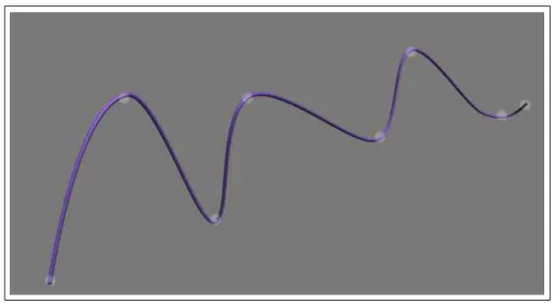
3.2.1.1.1 Cardinal Splines : A more intuitive way to create a cubic spline can be achieved through the Cardinal basis. Cardinal splines are much like Her-mite splines except that there is no need to define tangents at control points. Cardinal splines have the ability to calculate the tangents at control points from the coordinates of two adjacent points. As a result, only the manipulation of control points is necessary to define the spline shape.
A Cardinal spline segment is specified with four consecutive points. Only the middle points act as endpoints and the other two are used to calculate the
CHAPTER 3. 3D FUZZY TEXTURES 12
tangents of the endpoints (See Figure 3.2). At first, it may be thought that one must still deal with more than just the endpoints for slope calculation. However, considering that a final spline will have several segments, it can be seen that endpoints of one segment will be used for tangent calculation of the adjacent segments reducing the effort to define extra points for tangent calculation.
Figure 3.2: A cardinal spline segment
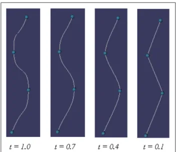
There is another parameter for cardinal splines called as the tension parameter that defines how tightly the spline fits the control points.
If we represent the parametric cubic function for the curve segment between endpoints pkan pk+1 with P (u), and the tension parameter as t, then, the
bound-ary conditions for the cardinal spline segment can be formulated as follows:
P (0) = pk, (3.3) P (1) = pk+1, P′(0) = 1 2(1 − t)(pk+1− pk−1), P′(1) = 1 2(1 − t)(pk+2− pk),
CHAPTER 3. 3D FUZZY TEXTURES 13
Then, we can derive the boundary conditions formulation as:
P (u) =hu3 u2 u 1i·MC · pk−1 pk pk+1 pk+2 , (3.4)
where the cardinal matrix is:
MC = −s 2 − s s − 2 s 2s s − 3 3 − 2s −s −s 0 s 0 0 1 0 0 , (3.5) and s = 1 − t 2 (3.6)
When the tension parameter t = 0, cardinal spline is called as the Catmull-Rom spline. In our experiments, we observed that a tension parameter value between 0.8 and 1.0 is the best value for curly and wavy hair styles. Tension parameter value between 0.1 and 0.3 is the best value for straight hair styles. See Figure 3.3 for the effects of tension parameter.
3.3
Growing Hairs within 3D Textures
After observing that Cardinal splines have the capability to model any kind of curly/wavy curve, it is necessary to find a way to convert spline geometry to texels information. Our aim is to construct a reference 3D texture that will reveal the hair details in final renderings. First, we form a 3D texture full of texels information. Then, this reference 3D texture will be mapped to global hair guides.
CHAPTER 3. 3D FUZZY TEXTURES 14
Figure 3.3: Effect of tension parameter for a Cardinal spline
3.3.1
Seed Hairs for the Unit Cube
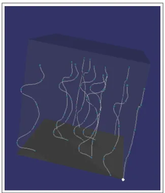
Generating the reference 3D texture starts with the definition of the seed hair strands for the unit cube. Since we use cardinal splines as hair geometry defini-tion, any desired curve may be defined in this step. Some example seed strands are shown in Figure 3.4.
CHAPTER 3. 3D FUZZY TEXTURES 15
After the seeds are introduced, all the remaining process is performed auto-matically. Our modeler program takes the seeds as guides and accepts them as clusters. In this way, we bind a clustering concept into the 3D texture as well. There are some user defined parameters for customizing the texel such as each cluster’s area, number of clusters and cluster density. According to the user de-fined parameters, our modeler program grows hair strands in the unit cube and waits for the command to convert the geometry information to texel information. During hair growing, there are two important steps for avoiding generation of regular patterns:
1. Placement of hair roots,
2. Clustering in the unit cube by deformations.
3.3.1.1 Placement of Hair Roots
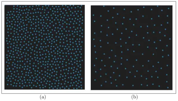
The first step in growing hairs in the reference unit cube is to decide about the positions of hair roots. We observe that positioning the hair roots is very impor-tant for breaking the regular unrealistic appearance. It must also be considered that random or very regular placement of hair roots results in aliasing artifacts during rendering if some ray casting algorithm is to be used. To overcome this problem, we place the hair roots in a Poisson disk sampling pattern.
Yellott [30] proposed that a Poisson disk distribution (a Poisson distribution with a minimum-distance constraint between points) is ideal for fixed-density (nonadaptive) sampling. According to his studies, Poisson disk distribution is also observed in retinal cells and using this pattern for high frequency data would yield more aliasing free images. More information on antialiasing patterns can be found in Mitchell [20].
In this work, we realized Poisson disk distribution with a ”dart-throwing” algorithm when placing the hair roots. Positions of the hair roots are generated randomly with a uniform distribution over the area being filled and each new point is rejected if it falls within a certain distance of any previously chosen
CHAPTER 3. 3D FUZZY TEXTURES 16
points, otherwise it is added to the pattern, and the process continues. Two example root placements with distance constraints d = 0.02 and d = 0.07 are shown in Figure 3.5. The dense one contains 707 hair roots and the coarse one contains 132 hair roots.
(a) (b)
Figure 3.5: Sample hair root placements for different Poisson distance con-straints: (a) d = 0.02; and (b) d = 0.07.
3.3.1.2 Clustering in the Unit Cube by Deformations
The second step for growing hairs within the unit cube is to fill in the seed clusters with hair strands. After the user sketches the guiding clusters, each cluster is copied in the unit cube as many as the user defined parameter numClusters. Only copying and placing with a Poisson distribution is not enough for getting convincing results. Curly or wavy hair contains so many clusters even within a one large cluster. Therefore, when copying the seed clusters, we deform them as to produce self similar clusters. Deformation of a seed cluster is performed by rotating its control points around the up vector axis with a random angle. Self similar clusters for cardinal splines given in Figure 3.4 can be seen in Figure 3.6.
CHAPTER 3. 3D FUZZY TEXTURES 17
Figure 3.6: Self similar clusters of seed hairs
3.4
From Cardinal Splines to Texels
The last step in constructing the reference texels is the conversion step. When generating the texels, it is necessary to determine the volume cells that each cardinal spline intersects. Whenever an intersection is discovered, it means that the density of that cell shall be increased by an amount equal to the hair strand’s opacity. This scalar will correspond to ρ (microsurface projected area) in Kajiya’s texel definition. By finding the intersection, we also have the chance to calculate and store the tangent at that point.
In scientific visualization, we usually get only the volume density information in a 3D array, and then it requires calculation of tangents by taking gradients in volume density. However, in our approach, we already have the surface geometry. Therefore finding the tangents simply reduces to calculation of the derivative of the parametric curve at the desired point. We are required to find the tangents since they will be used in rendering.
CHAPTER 3. 3D FUZZY TEXTURES 18
way to eliminate the unnecessary tests. It is extremely inefficient to traverse each volume cell and check that cell’s intersection with each hair strand.
We introduce a spline following algorithm named ”marching cells” to realize an optimization. Name is inspired from the well-known algorithm ”marching cubes”. Before stating the algorithm, we suggest a method for calculating the intersection of a cardinal spline with a texel.
3.4.1
Intersecting Cardinal Splines with Texels
Assuming that the unit cube is positioned at the origin without any deformations and the resolution of the unit cube is n3
for n ≥ 0, each side of the volume cell shall have the plane equation:
x = a or y = b or z = c, where a, b, c are the constants proportional to the cell indices.
Cardinal spline equation given in 3.4 may also be expressed as:
P (u) =hu3 u2 u 1i | {z } ~ U · ~ A ~ B ~ C ~ D , | {z } ~ Γ (3.7)
As ~Γ being the multiplication of the cardinal matrix MC with the knots vector.
Note that ~A, ~B, ~C and ~D are triples.
Then, we can write each component of the cardinal spline in the direction of the unit vectors as:
P (u)x·x = ~~ U · ~Γx·~x, (3.8)
CHAPTER 3. 3D FUZZY TEXTURES 19
P (u)z·z = ~~ U · ~Γz·~z,
Since the spline will intersect either the plane x = a or y = b or z = c, finding the intersection point reduces to solving the cubic equations:
(of the form m x3
+ n x2 + p x + r = 0) ~ U · ~Γx = a, (3.9) ~ U · ~Γy = b, ~ U · ~Γz = c,
Then, any numerical method can be applied for finding the intersection plane and the intersection point [25].
3.4.2
Marching Cells
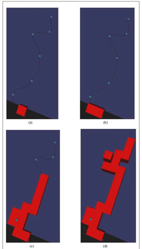
As stated before, main purpose of the algorithm is to reduce the intersection tests by following the cardinal splines through the unit cube. This enables only the calculation of intersections that are certain to occur. The algorithm is shown in Algorithm 1. The functions in the algorithm are simple 3D functions that test the existence of a point inside a cube except that F indSplineT exelIntersection(). The implementation details of this is given in Subsection 3.4.1. Figure 3.7 shows the marching cells algorithm for a cardinal spline during the conversion process. Red cells are the ones that were subject to march and converted to texel.
3.4.3
Antialiasing during Texel Conversion
Marching cells algorithm generates texels for each volume cell over the cardinal splines. However, spline curves are much thinner than a size of a volume cell. Therefore, aliasing problems are caused by the inadequate sampling of continu-ous information. Increasing the resolution of the unit cube along with a super-sampling process may be a solution but this solution will require high memory
CHAPTER 3. 3D FUZZY TEXTURES 20
Algorithm 1The Marching Cells Algorithm
1: procedure MarchingCells(hairs) 2: for all hairStrand ∈ hairs do
3: hairRoot ← getStrandRoot(hairStrand)
4: currentCell ← getCellF rom3DP oint(hairRoot) 5: strandEnded ← f alse
6: while strandEnded 6= true do
7: U pdateT exelInf o(currentCell, hairStrand)
8: isecP oint ← F indSplineT exelIntersection(currentCell, hairStrand) 9: nextCell ← getCellF rom3DP oint(isecP oint)
10: currentCell ← nextCell 11: if nextCell = N IL then 12: strandEnded ← true 13: end if 14: end while 15: end for 16: end procedure
17: procedure UpdateTexelInfo(cell, strand) 18: cellDensity ← cellDensity + strandOpacity
19: cellT angent ← cellT angent + strandT angent ⊲ Tangents are normalized 20: end procedure
CHAPTER 3. 3D FUZZY TEXTURES 21
Figure 3.7: Marching cells algorithm. (a)Marching starts at strand root; (b)texel conversion for two cells; (c) conversion is getting closer to end; and (d) completed conversion.
CHAPTER 3. 3D FUZZY TEXTURES 22
requirements and computational power. Instead, we apply a three dimensional convolution kernel to each texel during conversion.
We use Gaussian smoothing operator as the convolution operator. In our experiments, we observed that the size of the convolution kernel depends on the resolution of the unit cube, but 33
sized kernel is usually sufficient for unit cube resolutions up to 2563
.
An isotropic (i.e., circularly symmetric) Gaussian in 3D has the form:
G(x, y, z) = 1 2πσ2 ·e −x 2 +y2+z2 2σ2 , (3.10) For a 33
kernel, we obtain 27 filtering values. Therefore, when the conversion takes place, setting a volume cell’s texel information also affects 27 neighbor-ing volume cells’ texel information around it. We find this method extremely successful for eliminating the aliasing artifacts.
After these processes, cardinal spline geometry has been converted to texel information successfully. Rendered 3D fuzzy texture examples are presented in Chapter 7.
Chapter 4
Limitations of Single Level
Abstraction
This chapter aims at describing the limitations of the single level abstraction. As it is seen in the experimental results section, our 3D fuzzy texture model is successful at giving fine details to hair and fur. However, rendering of texels alone is not very useful when one is not able to map those texels onto a target object.
In our study, we first tried to construct a hair and fur modeling framework using only the 3D fuzzy textures. We offer some solutions for mapping problem of 3D fuzzy textures onto triangular meshes. Although these solutions are successful for some hairstyles, they are far from being a general solution for using our textures efficiently. However, the work explained here reveals the necessity for hybrid models for generic hair styles.
4.1
Cloth Simulation for 3D Texture Mapping
When fuzzy textures are considered directly as rendering primitives, the first problem to be faced is finding an easy mapping method. Conventional techniques require a lot of user interaction for mapping each corner of 3D texture volume
CHAPTER 4. LIMITATIONS OF SINGLE LEVEL ABSTRACTION 24
to a target object. Our solution accepts the target surface (human head for this case) as a triangular mesh which is the most common modeling primitive today and avoids 3D texture coordinate generation on target surface with a method taken from cloth simulation applied to hair modeling. We find this method very useful for short hair or fur. Since the fuzzy texture contains the necessary fine details, there is no need to model any perturbations.
In the following lines, we explain using cloth simulation for 3D fuzzy texture mapping step by step.
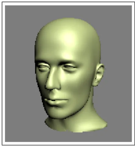
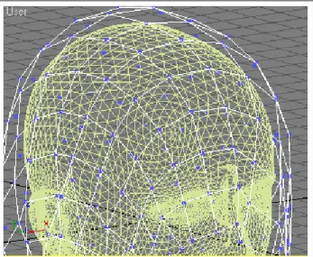
Step 1: An arbitrary triangular mesh acts as the target surface over which the hair shall be grown. Figure 4.1 shows such a model.
Figure 4.1: A triangular mesh head model
Step 2: A rectangular grid over the model is created. It is a plane whose vertices are connected with the well known mass-spring systems. This way it will behave as a deformable surface while intersecting with the head model. Friction constant for the head model is maximized and damping ratio for the springs is minimized since our aim is to find the intersections of the rectangular grid with the head model. We neither want the plane to skip over the surface nor to damp on the surface unnecessarily. Another approach would be projecting the head model to several planes. However, we found this method impractical especially for the problems we face with edges intersecting the projection planes. Figure 4.2 shows the initial state of deformable plane over the head model.
CHAPTER 4. LIMITATIONS OF SINGLE LEVEL ABSTRACTION 25
Figure 4.2: A rectangular grid over the model
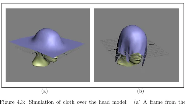
In this method, we can adapt the resolution of the rectangular grid without being dependent on the target surface complexity or geometry. In Figure 4.2, a 10 by 10 rectangular grid is over the target model. As soon as the system enters a stable state, we record the intersections of the rectangular grid with the target surface. In Figure 4.3, system’s states at some arbitrary times are shown.
(a) (b)
Figure 4.3: Simulation of cloth over the head model: (a) A frame from the simulation study; (b) steady state.
CHAPTER 4. LIMITATIONS OF SINGLE LEVEL ABSTRACTION 26
Figure 4.4: A closer look of the steady state at the top of the target surface
Step 3: The basic appearance and length to hair volumes are given at this point. An example short punk model is given in Figure 4.5. Polygon extrudes with rotations and transformations can be applied for getting the desired global shape. Note that it is not necessary to give the detailed curves at this level because it shall already be provided by the 3D fuzzy texture.
Figure 4.5: A short punky hair style
After this point, 3D textures shall be mapped to the extruded meta model which is straightforward. Rendering results with this method is presented in Chapter 7.
CHAPTER 4. LIMITATIONS OF SINGLE LEVEL ABSTRACTION 27
As stated before, trying to generate long hair with this method does not produce very good results. For a more flexible system, we need one more level of abstraction.
Chapter 5
Second Level of Abstraction
In this chapter, we suggest a method to combine the proposed 3D fuzzy texture with a second level of abstraction for human hair. Although 3D fuzzy textures are successful at giving fine detail to hair in a user controlled way, we observed that different hair styles, especially the long ones require a more flexible definition of hair clusters.
5.1
The Cluster Hair Model
The cluster hair model was introduced by Yang et al. [29]. Their suggestion is to represent human hair with a volume density model embedded within a generalized cylinder. The cluster model allows the design and styling of hair to be performed efficiently via generalized cylinders. Yang et al. modeled the details of hairs within the generalized cylinder by a randomly generated base density distribution map. This model especially enabled them interactive design and styling of long hair styles.
The cluster model was very successful at modeling long hair styles. However as they stated in their paper, the limitation of the cluster model is that modeling curly hair is almost impossible with this model since curly hair consists of a very
CHAPTER 5. SECOND LEVEL OF ABSTRACTION 29
large number of small clusters. Therefore it is not possible to approximate the volume properties of curly hair with clusters. Effort to make this would require hours of artist effort along with very long rendering times. Another drawback of the model was difficulty with estimating the effects of randomness parameters. The performance of the model was slow and they tried to improve it in a later work with a sweeping algorithm [28].
In this thesis, we propose a method to eliminate the problems of the current cluster models with our 3D fuzzy texture model. Since fuzzy textures are very successful at giving the required degree of curliness, a combination with a cluster model would result in successful modeling of complex hair styles.
5.2
Generalized Cylinders
There has been an extensive research on computational geometry to describe the geometric form of objects when a 2D contour is moved or swept along a 3D trajectory. The contour stands for the cross section of the object and the trajec-tory is for the axis. The most common particular cases of sweeping algorithms are translational sweeping and rotational sweeping. In translational sweeping an arbitrary 2D contour is translated along a curve. In rotational sweeping, the con-tour is rotated around an axis or equivalently moved along a circular trajectory. For further details of sweeping algorithms, readers may refer to Akman and Ar-slan’s paper [1]. Also, Bronsvoort and Klok [4] discussed the generalized cylinders along with a ray tracing algorithm. We use their notation for the definition of generalized cylinders in this study.
Generalized cylinders are defined by an arbitrary 2D contour and an arbitrary 3D trajectory along which to sweep it.
The 3D trajectory t can be defined in terms of a parametric function:
CHAPTER 5. SECOND LEVEL OF ABSTRACTION 30
tx, ty and tz trace out the trajectory for different values of u ranging from ui
to uf.
The 2D contour c to define the cross section can also be defined in terms of a parametric function:
c(v) = (cx(v), cy(v)), vi ≤v ≤ vf. (5.2)
Likewise, tracing out the contour is performed with different values of v rang-ing from vi to vf.
The contour itself is not enough for a sweeping to occur appropriately. Besides the given parametrizations above, its orientation at every point on the trajectory has to be specified. This requires to choose a local coordinate system for the contour at each point t(u) of the trajectory. It is necessary to define a coordi-nate system with the plane of the contour perpendicular to the trajectory, and the orientation of the contour in the plane following the local behaviour of the trajectory. A good choice of such a coordinate system is the Frenet frame. It is a good choice because it is independent of the coordinate system that the trajec-tory is defined. The Frenet frame is also independent of the parameterization of the trajectory. Its only dependency is on the local shape of the trajectory. The Frenet frame can be established by the following argument:
The vector ~t′(u) is in the direction of the tangential of t at t(u), the vector
~
t′′(u) is linearly independent of ~t′(u), and not being necessarily orthogonal to it.
~t′(u) and ~t′′(u) span the plane which is closest to points on the trajectory, in the
neighborhood of t(u). We use ~t′(u) and ~t′′(u) to form an orthogonal system of
unit vectors ( ~e1(u), ~e2(u), ~e3(u)) for the Frenet frame with origin at t(u) in the
order given in 5.4.
Unless otherwise stated, we omit the explicit dependence of t on u for simpli-fying the notation.
CHAPTER 5. SECOND LEVEL OF ABSTRACTION 31 ~ e1 = ~t′ ~t′ , (5.3) ~ e3 = ~ e1× ~t′′ e~1× ~t′′ , ~ e2 = ~e3×e~1, ~
e3 is orthogonal to the plane spanned by ~t′ and ~t′′. ~e2 is in the spanning plane
and directed towards the center of curvature at t.
These vectors provide the condition that the Frenet frame is independent of the coordinate system and parameterization of t [5].
For the generalized cylinder, it is the Frenet frame that determines the position of the contour at each point of the trajectory. Therefore, boundary condition for a generalized cylinder is obtained as:
~Γ(u, v) = ~t(u) + cx(v) ~e2(u) + cy(v) ~e3(u). (5.4)
See Figure 5.1 for a generalized cylinder with its trajectory and contours with associated Frenet frames.
5.3
Generalized Cylinders as Hair Clusters
Generalized cylinders are very efficient in defining the global shape of hair clus-ters. However, it is important to select the trajectory and the contour geometries appropriately. To make cluster definition as flexible as possible, we selected car-dinal splines as trajectories of generalized cylinders. Definition of carcar-dinal splines and their advantages in hair modeling is discussed in Chapter 3, so we will not go
CHAPTER 5. SECOND LEVEL OF ABSTRACTION 32
Figure 5.1: A generalized cylinder with some of its contours (reprinted from [4])
into the details in this chapter. We use circles for the 2D contour of generalized cylinders.
If we define a cardinal spline as described in equation 3.7, its normalized tangential at u can be obtained by:
~ T (u) = d ~P (u) du = h 3u2 2u 1 0i· ~Γ (5.5)
Then, we get the Frenet frame basis vectors as:
~ e1 = ~ T (u) T (u)~ , (5.6) ~ e3 = ~ e1× ~t′′ e~1× ~t′′ , ~ e2 = ~e3×e~1.
CHAPTER 5. SECOND LEVEL OF ABSTRACTION 33
cx(v) = R cos v, (5.7)
cy(v) = R sin v.
R being the radius of the cross sectional contour.
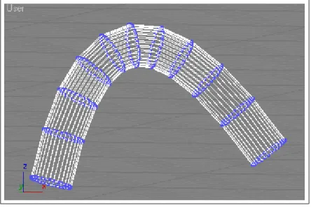
Now, we have all the parameters to obtain the boundary conditions for the generalized cylinder defined in equation 5.4. A generalized cylinder with its boundary vertices painted in blue can be seen in Figure 5.2
Figure 5.2: A generalized cylinder
5.4
Slicing of Generalized Cylinders
There are mainly two methods to approximate the volume characteristics of hair as explained in Chapter 2. One of them is using directly the volume data and ray cast it as Kajiya [12] and Perlin [24] did in the early works. The other one is to slice the volume as polygons and use the hardware support for blending them as Lengyel [14] introduced as shells method. The method used directly affects the rendering times. Direct volume rendering [16, 7] is a very costly method and we
CHAPTER 5. SECOND LEVEL OF ABSTRACTION 34
do not find it practical for the stated reason. We use slicing of volume data and try to approximate the volume with the help of transparent polygonal slices.
There can be many slicing schemes for the hair clusters depending on the type of the cluster geometry used. Wang et al. [28] sliced the hair clusters represented by generalized cylinders by the cross sectional contours of the trajectory. We find this method unpractical some cases especially at some viewing angles. Instead we slice the generalized cylinders with planes perpendicular to the cross sectional contour.
In our study, slicing of generalized cylinders is performed every time the view-ing angle changes. We calculate the nearest point on the circular contour that is subject to construct the slice edge and we form parallel polygonal slices in the direction of eye vector. Arc length between adjacent polygonal slices is taken to be the same for preventing high saturation around the nearest and the furthest slices.
Slicing distance is an important factor for the visual quality of rendered im-ages. According to our experiments, we observed that a slicing angle of 4 or 5 degrees is sufficient for getting good visual results. We also observed that after some point, it makes no difference how small the slicing angle is. We see the same effect of sampling distance in volume ray casting here. See Figure 5.3 for the slicing scheme.
5.5
Global Hair Cluster Placement
Generalized cylinders are excellent tools for giving the global shape of hair. Our system accepts hair clusters as generalized cylinders and converts them to polyg-onal slices as described in the previous section. To realize that and to be able to render hair and fur with other objects, we realized a simple scene graph compat-ible with Pixar’s RenderMan interface scene definition [27, 2].
CHAPTER 5. SECOND LEVEL OF ABSTRACTION 35
Figure 5.3: Slicing between the contours of a generalized cylinder
clusters required is reduced by a great amount with our approach thanks to 3D fuzzy textures. The need to generate curly hair styles with hundreds of clusters is also eliminated. An example global cluster placement can be seen in Figure 5.4.
CHAPTER 5. SECOND LEVEL OF ABSTRACTION 36
5.6
Mapping of Fuzzy Textures onto Slices
In Chapter 4, we stated the problems to be faced when 3D fuzzy textures are directly used as rendering primitives. In this section, we suggest to generate 3D texture coordinates for the cluster slices and map the fuzzy texture to these slices.
Today, every graphics card provides support for 3D textures. To be able to use this capability, every vertex of the textured polygon must be given a texture coordinate. This coordinate specifies the point in the 3D texture from where the data will be fetched. Texture coordinates of the fragments between the vertices are interpolated by the hardware.
Although it is common that 2D and 3D textures store color data, it has recently become popular to use textures for general purpose computational data storage [8]. At this point, texel information is just a 3D texture for the hardware and implementation of this data is application dependent. We derive a cylindrical mapping scheme for a 3D texture as follows.
We aim at deriving a projection function F () such that:
(s, t, r) = F (x, y, z), (5.8)
where (x, y, z) are the coordinates of points on the generalized cylinder. We map the reference texture such that data through its height is mapped along the trajectory of the generalized cylinder (i.e. cardinal spline in our case) and data through the horizontal slices is mapped to the cross sections of the cylinder (i.e cross sectional circles in our case).
Any point on our generalized cylinder can be expressed as P (θ, u) where θ is the circular cross section angle and u is the spline interpolator. According to the constraints above, the mapping function we derive turns out to be:
CHAPTER 5. SECOND LEVEL OF ABSTRACTION 37
Figure 5.5: Mapping of a 3D texture onto a generalized cylinder
(s, t, r) = (1, θ−7π/4π/2 , u), 7π/4 ≤ θ ≤ 2π (1, θ+π/4π/2 , u), 0 ≤θ ≤ π/4 (1 −θ−π/4π/2 , 1, u), π/4 < θ ≤ 3π/4 (0, 1 − θ−3π/4π/2 , u), 3π/4 < θ ≤ 5π/4 (θ−5π/4π/2 , 0, u), 5π/4 < θ < 7π/4 (5.9)
The generalized cylinder mapping for a 3D texture can be seen in Figure 5.5.
As a result, we succeeded in mapping 3D fuzzy textures onto global hair clus-ters. Therefore, limitation of mapping problems faced in one level of abstraction and limitation of modeling only straight hair in the cluster hair model is avoided.
Chapter 6
Rendering
This chapter describes the rendering architecture we suggest for the cluster hair model combined with 3D fuzzy textures. Besides realizing some algorithmic op-timizations to improve rendering times, we try to utilize the new programmable shader capabilities of current generation GPUs.
6.1
System Overview
In the previous chapters, we explained our proposal for hair modeling. To be able to generate images of these models, we need a stable renderer along with an appropriate scene definition. For storing the scene definition, we developed a simple scene graph compatible with Pixar’s RenderMan Interface Scene Hierarchy.
Input to the system is a scene definition consisting of hair and non-hair objects and the 3D fuzzy texture that holds the texels information. The output is a rendered image. As stated before, scene definition is implemented by a scene graph.
A scene graph is simply a tree structure that holds the scene objects in a hierarchical way. Scene graphs are very good abstractions of large scenes with a lot of objects. Through this abstraction, data model becomes independent of the
CHAPTER 6. RENDERING 39
rendering system used. Our scene graph makes use of an abstraction in the level of global hair clusters and other objects that are non-hair.
When the system starts, it first reads the modeled and saved scene before. During the parsing process, scene graph is constructed. At this step, hair nodes and non-hair nodes are realized by the system. Then 3D fuzzy textures associated with the hair nodes that are loaded. During scene traversal, slicing of global hair clusters along with 3D texture coordinate generation are performed by hair slicer and sliced polygonal data along with 3D fuzzy textures are directed to the hair renderer. Meanwhile, if a nonhair object is encountered during scene traversal, it is directed to non-hair renderer. After all the scene is traversed and rendering is completed, both of the renderers’ outputs are delivered to image compositor. Here, final blending operations are performed and the output image is constructed. The process diagram of the whole system is shown in Figure 6.1. In the following lines, hair rendering and image composition processes will be detailed.
6.1.1
Hair Renderer
After the global hair clusters are sliced by hair slicer, polygonal slices are fed into the hair renderer. There are two main steps in our hardware hair rendering algorithm;
1. Rendering of polygonal slices and insertion to a sorted map,
2. Creation and rendering of meta textures from sorted fragments map.
6.1.1.1 Rendering of Slices
Initially all the polygonal slices are set to be totally transparent with no color information. All the polygon vertices have their 3D texture coordinates assigned at this stage. First, 3D fuzzy texture is bounded as the active texture. We bound this texture as alpha texture and consider the density information for each texel as
CHAPTER 6. RENDERING 40
CHAPTER 6. RENDERING 41
Figure 6.2: The framework for the slice rendering process
opacity of the texel. Then all the polygonal slices are rendered to the frame buffer with hardware blending disabled and depth testing enabled. However, after each polygon is rendered, we perform some post operations for correct depth sorting and blending. As soon as a polygonal slice is rendered to the frame buffer, we read its alpha channel from the color buffer and its depth information from the depth buffer into two separate textures. Then, taking each rendered fragment’s depth value as a key, we insert the rendered alpha map into a sorted map and clear the color and depth buffers. This way, we guarantee that the map contains the fragments in a depth sorted order. In fact, we realize a kind of ray casting algorithm in scan line hardware here. In ray casting, it is not necessary to think about depth sorting since the casted ray already visits the volume cells from front to back order. Process model for slice rendering can be seen in Figure 6.2.
CHAPTER 6. RENDERING 42
Figure 6.3: Meta textures rendering process model
6.1.1.2 Creation and Rendering of Meta Textures
After all the slices are rendered and inserted into the sorted fragments map, we create new meta textures for all the sorted slices existing in the sorted fragment map.
Then, these textures are rendered as view port sized quads with depth test-ing and blendtest-ing disabled. At this stage, we bind our hair shadtest-ing vertex and fragment shaders and send them the necessary data. After this point we use the frame buffer as a temporary render target and it always holds the latest state of the accumulated color and opacity data of hairs. Within a feedback loop, a final texture unit is updated from the frame buffer and blended with the hair shading calculations in the fragment shader. When all the textures are rendered, the final texture holds the rendered hair texture and sends it to image compositor. Process model of meta textures rendering can be seen in Figure 6.3.
CHAPTER 6. RENDERING 43
Figure 6.4: Non-hair rendering process model
6.1.2
Non-Hair Renderer
Non-hair renderer is simply acts as a scan line renderer with depth testing enabled. After all the non-hair objects are rendered to frame buffer, this renderer copies the frame buffer content to a texture and sends it to image compositor. Figure 6.4 gives non-hair rendering process model.
6.1.3
Image Compositor
When hair renderer and non-hair renderer feed their output textures to image compositor, image composition shader programs are bounded. Non-hair texture is sent to the fragment shader and hair texture is rendered as a view port quad. For each fragment of the hair texture, fragment processors work with the loaded composition program and blend the fragments with the non-hair texture. After this stage, frame buffer contains the final rendered image. See Figure 6.5 for the process model.
CHAPTER 6. RENDERING 44
Figure 6.5: Image composition process model
6.2
Shading
There have been many research in computer graphics to understand the bidirec-tional reflection distribution function (BRDF) of human hair fibers. There are some primitive ad hoc methods as well as the experimental studies.
The most common hair illumination model up to date has been the Kajiya and Kay [12] model because of its simplicity and convincing visual results. They suggested diffuse and specular components for the hair fibers by accepting the hair as a cylindrical surface.
To our knowledge, the most recent work on the experimental studies is the one carried at Stanford University by Marschner et al. [17]. Their work reveals some unknowns about the human hair fibers’ BRDF. Especially, they emphasize the importance of the second specular component for approximating the reflection characteristics of human hair. However, the model they propose is very costly and impractical for real-time purposes for now. Kajiya and Kay’s model for cylindrical surfaces and hair is more applicable to current applications. Therefore, we shall use their lighting model for hair illumination.
We can separate the fundamental components of hair illumination as diffuse and specular. The diffuse component is derived essentially from the Lambert
CHAPTER 6. RENDERING 45
shading model applied to a very small cylinder. The specular component is an ad hoc model similar to the Phong reflection model that has been modified for cylindrical surfaces. According to Kajiya and Kay’s model, the diffuse component used for hair illumination is:
Ψdif f use = Kd·sin(~t,~l), (6.1)
where Kd is the diffuse reflection coefficient, ~t is the hair tangent and l is the
lighting vector from the illuminated point on the hair to the light source. sin(~t,~l) is the sine between the light and tangent vectors. The specular component is:
Ψspecular = ka((~t · ~l)(~t · ~e) + sin(~t,~l) sin(~t, ~e))p, (6.2)
where ka is some specular reflection coefficioent, ~e is the vector pointing to the
eye and p is the Phong exponent specifying the sharpness of the highlight.
We realize these calculations for every hair fragment in the fragment processor of the graphics cards. For the details of the illumination model, readers may refer to [12].
Chapter 7
Experimental Results
7.1
Visual Results For 3D Fuzzy Textures
Figure 7.1 shows a 3D texture filled with straight texels information, this image is nothing more than implementation of [12]. Figure 7.2 shows a 3D fuzzy texture without clustering in unit cube. Figure 7.3 shows the effect of clustering in unit cube for fuzzy textures. Figure 7.4 render results for multiple fuzzy textures.
CHAPTER 7. EXPERIMENTAL RESULTS 47
Figure 7.1: 3D texture with straight texels
CHAPTER 7. EXPERIMENTAL RESULTS 48
Figure 7.3: A 3D fuzzy texture with clustering in the unit cube
CHAPTER 7. EXPERIMENTAL RESULTS 49
7.2
Visual Results for Single Level Abstraction
with Fuzzy Textures
Figure 7.5 illustrate the rendering obtained with single level abstraction and mapping results when cloth simulation is used as an intermediate tool.
CHAPTER 7. EXPERIMENTAL RESULTS 50
7.3
Visual Results for Two Level Abstraction
with Fuzzy Textures
Figure 7.6 shows a generalized cylinder mapped with a 3D fuzzy texture. It consists of one cluster and the mapped 3D fuzzy texture’s resolution is 643
. The image resolution is 256 by 256 and the rendering time is 45 seconds.
Figure 7.7 shows a sphere with global hair clusters grown and fuzzy textures mapped. It consists of one cluster and the mapped 3D fuzzy texture’s resolution is 643
. No low-pass filtering was applied to the fuzzy texture during texel conversion process. Therefore, some aliasing artifacts are obvious in the rendered image. The image resolution is 256 by 256 and the rendering time to obtain that image is 47 seconds.
Figure 7.8 shows a head model with hairs grown. There are two clusters on the head. Finer details are all given by the 3D fuzzy texture. Fuzzy texture resolution is 643
and rendering time is 2.5 minutes for that 256 by 256 image.
Figure 7.9 shows a front facing head model with long wavy hairs. There are five clusters on the head. 3D Fuzzy texture resolution is 643
and rendering time is 35 minutes for that 256 by 256 image.
Figure 7.10 shows a head model with long wavy hairs rendered from back. There are five clusters on the head. 3D Fuzzy texture resolution is 643
and ren-dering time is 40 minutes for that 256 by 256 image.
CHAPTER 7. EXPERIMENTAL RESULTS 51
Figure 7.6: Generalized cylinder mapped with a 3D fuzzy texture
CHAPTER 7. EXPERIMENTAL RESULTS 52
Figure 7.8: A head model with fine detailed hair grown with fuzzy textures
CHAPTER 7. EXPERIMENTAL RESULTS 53
Figure 7.10: A head model with long wavy hair from back
7.4
Performance Considerations
The rendering system described works fine with image sizes up to 64 by 64 pixels. However, when the image size gets larger, we face with memory shortage because of the map used for holding the sorted fragments. Shortage of memory results in page swapping and this swapping process makes the rendering times unnecessarily very high. To eliminate this problem, we realize an optimization like Pixar’s REYES architecture [2] performs. This optimization is also suggested by Wang and Yang [28] as dynamic pixel buffering. To reduce the amount of data to be sorted, viewport is divided into regions called buckets. There becomes as many render passes as the number of buckets, but this is much preferable to page swapping performed by the operating system. With this method, sorted fragment map size is reduced and page swapping is prevented.
One other optimization we performed is for multiple render passes. For each bucket, there is no need to render all the polygonal slices. Therefore, we only render the slices that are in the viewing frustum of the current bucket.
CHAPTER 7. EXPERIMENTAL RESULTS 54
Besides the algorithmic optimizations stated above, there are also optimiza-tion opportunities that can be done using the graphics hardware. The main bottleneck of the rendering system described above is the Copy to Texture pro-cesses. With the evolution of hardware, this functionality becomes faster and faster every day. The first implementation for getting the frame buffer content to a texture was to copy it directly. However, this is the slowest method. Then, the method called as render to texture appeared. For this purpose, a new buffer called p-buffer was introduced by NVIDIA [22]. This buffer aimed at speeding up texture copying by binding itself to the frame buffer but this method did not meet the expectations either. Recently, the problem seems to be solved by the concept Frame Buffer Objects (FBOs). These objects are seen as render targets by the video card and direct offline rendering becomes possible with this new hardware concept. In our study, we did not use FBOs since some cards still does not support it. However, implementation with FBOs would make the rendering process much faster.
We performed our tests on a notebook with a Pentium-IV with 1 GB of RAM. The graphics card used is ATI-X300 with 256 MB of memory. Even with a note-book, we obtained the rendering in Figure 7.8 in 2.5 minutes. When compared to other methods in the literature, to our knowledge, our method is the only one that enables cluster hair rendering within a single CPU system in minutes. We obtain this speed up thanks to the proposed rendering architecture and the fuzzy texture model since it reduces the high number of clusters taking the responsibility for giving fine details for hair.
![Figure 5.1: A generalized cylinder with some of its contours (reprinted from [4]) into the details in this chapter](https://thumb-eu.123doks.com/thumbv2/9libnet/5786838.117615/44.892.284.604.166.503/figure-generalized-cylinder-contours-reprinted-details-chapter.webp)