T K 7 ^ 8 2
■S6S
e ? 9
A DISSERTATION
SUBMITTED TO THE DEPARTMENT OF ELECTRICAL AND ELECTRONICS ENGINEERING
AND THE INSTITUTE OF ENGINEERING AND SCIENCE OF BILKENT UNIVERSITY
IN PARTIAL FULFILLMENT OF THE REQUIREMENTS FOR THE DEGREE OF
DOCTOR OF PHILOSOPHY
By
Engin Erzin
September 1995
ί -ѵз e s s
dissertation for the degree of Doctor of Philosophy.
A. Enis Çetin, Ph. D. (Supervisor)
I certify that I have read this thesis and that in my opinion it is fully adequate, in scope and in quality, as a dissertation for the degree of Doctor of Philosophy.
Orhan Arikan, Ph. D.
I certify that I have read this thesis and that in my opinion it is fully adequate, in scope and in quality, as a dissertation for the degree of Doctor of Philosophy.
dissertation for the degree of Doctor of Philosophy.
I certify that I have read this thesis and that in my opinion it is fully adequate, in scope and in quality, as a dissertation for the degree of Doctor of Philosophy.
Miibeccel Demirekler, Ph. D.
Approved for the Institute of Engineering and Science:
____________________ __________________________
Mehmet Baray, Ph. D /
NEW METHODS FOR ROBUST SPEECH RECOGNITION
Engin Erzin
Ph. D. in Electrical and Electronics Engineering
Supervisor:
Assoc. Prof. Dr. A. Enis Çetin
September 1995
New methods of feature extraction, end-point detection and speech enhcince- ment are developed for a robust speech recognition system.
The methods of feature extraction and end-point detection are based on wavelet analysis or subband analysis of the speech signal. Two new sets of speech feature parameters, SUBLSF’s and SUBCEP’s, are introduced. Both parameter sets are based on subband analysis. The SUBLSF feature parameters are obtained via linear predictive analysis on subbands. These speech feature parameters can produce better results than the full-band parameters when the noise is colored. The SUBCEP parameters are based on wavelet analysis or equivalently the m ultirate subband analysis of the speech signal. The SUBCEP parameters also provide robust recognition performance by appropriately deemphasizing the frequency bands corrupted by noise. It is experimentally observed that the subband analysis based feature parameters are more robust than the commonly used full-band analysis based parameters in the presence of car noise.
The a-stable random processes can be used to model the impulsive nature 111
of the public network telecommunication noise. Adaptive filtering are developed for Q-stable random processes. Adaptive noise cancelation techniques are used to reduce the mismacth between training and testing conditions of the recognition system over telephone lines.
Another important problem in isolated speech recognition is to determine the boundaries of the speech utterances or words. Precise boundary detection of utterances improves the performance of speech recognition systems. A new distance measure based on the subband energy levels is introduced for endpoint detection.
Keywords : Speech recognition, linear prediction, endpoint detection, speech enhancement, subband decomposition, wavelet trans form, line spectrum frequencies, a-stable distributions.
KONUŞMA TANIMA İÇİN GÜRÜLTÜYE DAYANIKLI YENİ
YÖNTEMLER
Engin Erzin
Elektrik ve Elektronik Mühendisliği Bölümü Doktora
Tez Yöneticisi:
Doç. Dr. A. Enis Çetin
Eylül 1995
Dayanıklı konuşma tanıma sistemleri için öznitelik parametrelerinin elde edilmesi, sözcük sınırlarının belirlenmesi ve konuşma iyileştirilmesi alanlarında yeni yöntemler geliştirilmiştir.
Öznitelik parametrelerinin elde edilmesi ve sözcük sınırlarının belirlenmesi yöntemleri altbant analizine dayalı biçimde geliştirilmiştir. Altbant analizine dayalı iki yeni konuşma öznitelik parametre vektörü (SUBLSF ve SUBCEP) oluşturulmuştur. SUBLSF öznitelik parametrelerini elde etmek için konuşma işareti alt ve üst bantlara ayrılır. Her iki' bant için doğrusal öngörü analizi yapılır ve bu analizlerden elde edilen Çizgisel Spektrum Frekansları birleştirilerek SUBLSF öznitelik vektörü oluşturulur. Diğer öznitelik parametre vektörü, SUBCEP, dalgacık analizi veya eşdeğer anlamda altbant analizi kullanılarak oluşturulur. SUBCEP parametreleri gürültülü bantları bastırarak dayanıklı bir başarım sağlamışlardır. Yapılan deneyler sonunda araç gürültüsü altında altbant analizi ile elde edilen öznitelik parametrelerinin yaygın olarak kullanılan tam-bant
parametrelerinden daha dayanıklı olduğu görülmüştür.
Telefon kanallarındaki gürültünün modellenmesinde a-kararlı rasgele süreçler kullanılabilir. o;-kararlı rasgele süreçler için geliştirilen uyarlamalı süzgeçler gürültülü konuşmanın iyileştirilmesinde kullanılmış ve konuşma tanım a başarımı artırılm ıştır.
Dayanıklı konuşma tanım a sistemlerinde bir diğer önemli problem de sözcük sınırlarının belirlenmesidir. Sözcük sınırlarının hatasız belirlenmesi konuşma tanım a başarımmı artırmaktadır. Sözcük sınırlarını belirlemeye yönelik, konuşma işaretinin altbant enerji değerlerine bağlı, yeni bir uzaklık ölçüsü sunulmuştur.
A nahtar sözcükler: Konuşma tanıma, doğrusal öngörü, sınır belirleme,
konuşma iyileştirme, altbant ayrışımı, dalgacık dönüşümü, çizgisel spektrum frekansları, a-kararlı dağılımlar.
I would like to express my deepest gratitude to Dr. A. Enis Çetin for his supervision, guidance, suggestions and encouragement throughout the development of this thesis, and also for that he introduced me to the signal processing society in various international conferences from which I gained experience and motivation.
I would like to thank to Dr. Orhan Ankan, Dr. Yasemin Yardımcı, and my project group in METU, especially to Prof. Dr. Miibeccel Demirekler, Burak Tüzürı and Bora Nakipoglu, for their valuable technical support and discussions.
I like to acknowledge to ASELSAN (Military Electronics Industry Inc.) for their financial supports to our research.
Thanks to all my friends who have been with me during my Ph.D. study, especially to Fatih, Gem, Aydın, Suat, and Ayhan for their morale support and friendship, and to Tuba, Zafer, and Esra for making me smile even if I feel so desperate and for their friendship.
Finally, it is a pleasure to express my sincere thanks to my family for their continuous morale support throughout my graduate study.
A b stract iii
Ö zet V
A cknow ledgm ent vii
List o f Figures xi
List o f Tables xiv
1 IN T R O D U C T IO N 1
1.1 Linear Predictive Modeling of Speech 4 1.1.1 Linear P re d ictio n ... 7
1.1.2 Line Spectral Frequencies 11
1.2 Speech R ecognition... 12
1.2.1 Hidden Markov Model (HMM) 14
1.3 Speech Recognition Research in T u rk e y ... 24
2 LINE SP E C T R A L FREQ UENC IES IN SPEECH R E C O G N I
T IO N 26
2.1 LSF Representation of S p e e c h ... 27
2.2 LSF Representation in Subbands for Speech R e c o g n itio n ... 29
2.2.1 Performance of LSF Representation in Subbands 31 2.2.2 Conclusion... 32
3 W AVELET ANALYSIS FOR SPEECH R EC O G N ITIO N 34 3.1 Subband Analysis based Cepstral Coefficient (SUBCEP) Repre sentation 35 3.1.1 Frequency Characteristics of the Iterated Filter Bank Structure ... 41
3.2 Simulation S t u d i e s ... 43
3.2.1 Experiments over the TI-20 Database 44 3.2.2 Performance over the Data Set Recorded in a C a r ... 47
3.2.3 Conclusion... 48
4 A D A P T IV E NO ISE C A N C ELIN G FOR R O B U ST SPEEC H R E C O G N IT IO N 49 4.1 Adaptive Filtering for non-Gaussian Stable P ro c e s se s... 50
4.1.1 Adaptive Filtering for a-stable Processes... 52
4.2 Adaptive Noise Canceling for Speech R e co g n itio n ... 55
4.3 Simulation S t u d i e s ... 58
5 W AVELET ANALYSIS FOR E N D PO IN T D E T E C T IO N OF ISOLATED U T T E R A N C E S 61 5.1 A New Distance Measure based on Wavelet Analysis 62 5.2 Simulation E x a m p le s... 65
5.4 The energy measure of the noise free utterance “four” is plotted in (a). The new distance measure and the energy measure for different SNR levels are plotted in (b) and (c), respectively. The solid (dashed) [dash-dotted] {dotted}line corresponds to 30 dB (15
dB) [10 dB] {8 dB}noise level. 66
5.5 The energy measure of the noise free utterance “start” is plotted in (a). The new distance measure and the energy measure for different SNR levels are plotted in (b) and (c), respectively. The solid (dashed) [dash-dotted] {dotted}line corresponds to 30 dB (15
dB) [10 dB] {8 dB)noise level. 67
5.6 The recording of the Turkish word “hayır : / h a y i r / ” (no) inside a car is plotted in (a), the new distance measure and the energy measure are plotted in (b) and (c), respectively... 68 5.7 (a) The new measure Dk for a utterance recorded inside a car, (b)
the histogram of the new measure Dk- 69 5.8 Flowchart for the endpoint algorithm. 71 5.9 The distance measure Dk for the Turkish word “'evet” and the
end-point locations that are detected by the algorithm. 72 B.l Transient behavior of tap weight adaptations in the NLMP,
NLMAD, LMAD, LMP and LMS algorithms for AR(1) process. . 82 B.2 Transient behavior of tap weight adaptations in the NLMP,
NLMAD, LMAD, LMP and LMS algorithms for AR(2) process. . 83 B.3 The adaptation performances of LMAD, NLMAD and NLMP
2.1 Recognition rates of SUBLSF, MELCEP and LSF representations
in percentage. 32
3.1 The average recognition rates of speaker dependent isolated word recognition system with SUBCEP and MELCEP representations for various SNR levels with Volvo noise recording. 45 3.2 The average recognition rates of speaker dependent isolated word
recognition system with SUBCEP and MELCEP representations for various SNR levels with Skoda noise recording.
3.3 The performance evaluation of speaker independent isolated word recognition system with SUBCEP and MELCEP representations for various SNR levels with Volvo noise recording.
46
16 3.4 The performance evaluation of speaker independent isolated word
recognition system with SUBCEP and MELCEP representations for various SNR levels with Skoda noise recording. 47 4.1 The average recognition rates of speaker dependent isolated word
recognition system with SUBCEP and MELCEP representations for various SNR levels with a-stable noise (a = 1.95). 59 4.2 The average recognition rates of speaker dependent isolated word
recognition system with SUBCEP and MELCEP representations for various SNR levels with a-stable noise (a = 1.5). 59
4.3 The average recognition rates of speaker dependent isolated word recognition system v.dth SUBCEP and MELCEP representations for various SNR levels with a-stable noise (a = 2.0). 60 A.l The angular offset factors which are used in simulations 80 A.2 Codebook sizes for each subvector at different r a t e s ... 80 A.3 Spectral Distortion (SD) Performance of our method 80 A.4 Spectral Distortion (SD) Performance of the Vector Quantizers
IN T R O D U C T IO N
Speech is the central component of the field of telecommunications, as it is the most effective interface between human beings. How humans produce, process and recognize speech has been an active research area since the classical ages [1]. Advances in digital signal processing technology bring new challenges to the speech processing with wider application areas. Today the essential application areas of speech processing are compression, enhancement, synthesis and recognition [2].
The successful modeling of the vocal tract with the linear predictive (LP) analysis techniques brought simple and effective solutions to the speech coding and synthesis [3, 4]. Lower bit rates, acceptable quality and security are rather important objectives that are achieved in a satisfactory way with linear prediction of speech signals.
Although the speech production system is successfully modeled, the human perception and recognition system is not well understood [5]. The first experiments regarding human speech recognition was done by Harvey Fletcher in early 19th century. These recognition tests were in the form of an empirical probabilistic analysis of speech recognition scores obtained from a series of listening experiments. Flecther used the word articulation in the perceptual context to mean the probability of correctly identifying nonsense speech sounds.
Human phone recognition rate for nonsense consonant-vowel-consonant syllables, under best conditions, was reported to be 98.5% [1, 6].
As the speech is becoming an important interface between human beings and machines, speech recognition stands as an important cornerstone of the speech processing. In the last 20 years, considerable progress has been achieved in this field. However, in terms of linguistic, natural language and understanding, speech recognition is a complicated application area, but when the dimensions are reduced, such as limited vocabulary and context, reliable recognition systems can be formed [7].
Automation of operator services, stock quotation services and voice control on mobile telephones can be considered as the current application areas of the limited vocabulary speech recognition systems.
In a recent review [8] on the challenges of spoken language systems by the leading authors in speech recognition field, the robustness in speech recognition is defined as minimal graceful degradation in performance due to changes in
input conditions caused by different microphones, room acoustics, background or channel noise, different speakers or other small systematic changes in the acoustic signal. At present, one of the major drawback of speech recognition systems is the
robustness. Their performance degrades suddenly and significantly with a minor mismatch between training and testing conditions [9]. Although signal processing strategies carry out some progress for more robust systems [10, 11, 12], the key point is to understand the many sources of variability in speech signal better for improving robustness. Variability is typically due to the speaker and the nature of the task, the physical environment, and the communication channel between user and the machine.
In this thesis, the sources of variability in car environment and telephone channels will be addressed and the methods on feature extraction, end-point detection and speech enhancement will be investigated for a robust speaker independent isolated word recognition system. In most cases, background noise is modeled as additive stationary perturbation which is uncorrelated to the speech signal. With this assumption, we tried to construct robust recognition systems in the presence of car noise and telephone channel noise. The current research
in robust speech recognition includes the car noise and the telephone channel environment due to the practical importance of these application areas [13, 14]. T hat is the main reason, these environments are considered in this thesis. In this chapter, vocal tract modeling and a speech recognition system based on the Hidden Markov Modeling (HMM) structure are reviewed.
In Chapter 2, robust feature extraction in subbands with LP analysis is investigated. Subband analysis is employed in order to separate the noisy and noise-free bands in the presence of car noise. The performances of the LSF’ representation and the cepstral coefficient representation of speech signals are comparable for a general speech recognition system [34, 35]. However, we obtain the SUBLSF feature parameters by first dividing the speech signal into low and high frequency bands, and then a linear predictive analysis will be performed on each subband. Consequently, the resulting two sets of LSF parameters are combined to form the SUBLSF feature parameters.
M ultirate signal processing based feature extraction is presented in Chapter 3. The new feature set, SUBCEP, is obtained from the root-cepstral coefficients derived from the wavelet analysis of the speech signal [37]. The performance of the new feature representation is compared to the mel scale cepstral representation (MELCEP) in the presence of car noise. The SLIBCEP parameters are realized in a computationally efficient manner by employing fast wavelet analysis techniques. Also, in the root cepstral analysis a fixed root value is used [13]. On the other hand the frequency bands are weighted by the proper selection of pi values. This increases the robustness of the speech feature parameters against the colored environmental noise. Therefore, our main contributions to the derivation of SUBCEP parameters are the subband decomposition based time-frequency analysis, and the weighted root nonlinearity.
Chapter 4 will cover the adaptive filtering type enhancement strategies which are applied to speech recognition system. The o-stable random processes are used to model the impulsive nature of the public network telecommunication noise [45]. Recently, adaptive filtering techniques are developed for a-stable random processes [48, 49]. In Chapter 4, we mainly investigate some adaptive noise cancelation structures to eliminate the mismatch between training (noise-free training) and testing conditions of a speech recognition system for telephone
channel conditions.
In Chapter 5, the new distance measure for end-point detection based on the subband energy levels are presented. To determine the boundaries of the speech utterances or words is an important problem in isolated speech recognition. The energy measure and the zero-crossing rate are the widely used distances in endpoint detection algorithms [55]. They perform fairly well at high SNR levels, however their performance degrades drastically in many practical cases, such as car noise which is usually concentrated at low frequency bands. Instead of using the full-band energy a me/-frequency weighted energy measure is introduced in Chapter 5. In order to obtain the me/-scale frequency division in a computationally efficient manner, multirate signal processing based methods are employed.
Conclusions and discussions are given in Chapter 6.
In the following sections, the LP modeling of the speech signal is introduced and LP feature parameterization of the speech signal is given. Also, a general overview of a speech recognition system is given.
1.1
Linear P r e d ic tiv e M odeling o f S p eech
The speech production system has been successfully modeled by the linear predictive (LP) analysis which found large application areas that cover coding, synthesis and recognition. Computationally efficient and accurate estimation of the speech parameters, such as pitch, reflection coefficients, and formant frequencies, makes this method a widely used one [4].
The basic idea of linear predictive (LP) analysis is that the current speech sample, s(n) at time instant n can be estimated as a linear combination of past
p speech samples, such that
s { n ) — Y^ais{n - i) + Gu{n), (1.1)
1=1
analysis frame and u(n) is the excitation with gain G. By expressing Equation 1.1 in the z-domain, we write the relation
S{z) = Y^aiZ 'S{z) + GU{z)
¿=1
(
1.
2)
leading to the transfer function 5(z)
H{z) =
GU(z) i - E L i « . · ^ - · (1.3)
Applying an error minimization criterion over a block of speech data one can come up with a set of predictor coefficients for an all-pole, linear, time-varying filter model.
Pitch
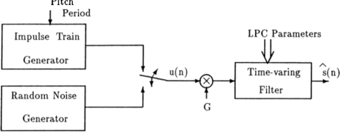
Figure 1.1: LP Vocoder Synthesizer.
A simple model of speech can be constructed using a linear predictor. For
example, in LP vocoders (voice-coders) [4], the all pole linear predictor is excited by c[uasi-periodic pulses during voiced speech, and by random noise during unvoiced speech to generate synthetic speech.
The basic block diagram of an LP vocoder is shown in Figure 1.1. In LP vocoders the human vocal tract is modeled as an all-pole linear predictor as in Equation (1.3), where A{z) is a minimum phase polynomial. In vocoders the coefficients of the filter are obtained by LP analysis which is carried out over speech frames of duration 20 to 30 msec. It is assumed that the statistical characteristics of the speech signal do not vary during a speech frame. Speech
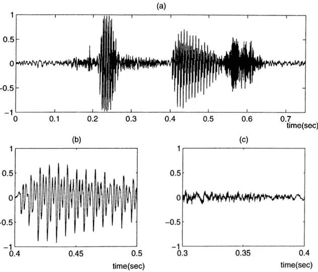
frames are first characterized as voiced or unvoiced frames which are modeled differently. As it can be seen in Figure 1.2-(b) the speech signal is almost periodic in voiced regions. The “period” is called the pitch of the voiced frame. In unvoiced speech the time series exhibit such a pattern as shown in Figure 1.2-(c). It is assumed that the vocal tract or the linear filter is excited by an impulse train whose period is the same as the pitch value for voiced speech and by random noise for unvoiced speech. Voiced/unvoiced decision, pitch period calculation, can be carried out either in the time or the frequency domains.
0.7
time(sec)
Figure 1.2: (a) An example of a speech signal corresponding to the Turkish
utterance “sıfır”, (b) A voiced segment of the speech signal, (c) An unvoiced segment of the speech signal.
In the next section a commonly used LP analysis procedure is described for determining the filter coefficients, a^’s.
1.1.1
Linear P r e d ic tio n
The estimate s(n) of the speech signal s(n) is defined as the linear combination of past speech samples
p
= J2 ^ks{n - k), (1.4)
k = l
by the speech model of Equation (1.3), Consequently the prediction error e{n) is defined as,
p
e(n) = s{n) — s{n) = s{n) — ^ aks{n — k) (1.5) A := l
with the error transfer function
(1.6)
A r= l
If s{n) were actually generated by a linear system as in Figure 1.1, then the prediction error, e(n), would be equal to Gu{n), the scaled excitation.
The basic problem of the LP analysis is to determine the predictor coefficients, {a^:}, directly from the speech signal. Since the spectral characteristics of the speech signal vary over time, the predictor coefficients at time instant, n, must be estimated from a short segment of the speech signal occuring around the same time instant. A set of predictor coefficients can be found by minimizing the mean-squared prediction error over a short speech frame.
Let us define short-time speech and error segments at time n as s„(m) = s(n -f m)
e„(m) = e(n-l-m ), m = 0 ,1 ,2 ,..., - 1, and try to minimize the mean-squared error signal at time n
(1.7)
(1.8)
which can be written as K = T , 1 2 Sn{m) - akSn{m - k) k=l (1.10)
Equation (1.10) can be solved for the predictor coefficients by differentiating En with respect to each ak and setting the results to zero,
dEn dak = 0, A: = l , 2 , . . . , p giving Y s„(m - ¿)s„(m) = Y o k Y Sn{m. - i)s„(m - A:). m rn (1.11) (1.12)
By defining k) = s„(m — — k) as the short-time covariance of
Sn{m), Equation (1.12) can be expressed in the compact form
^n(«',0) = Y d k ^ n { i ,k ) , i = 0,1,2, . . , p - 1 /:=!
(1.13) which describes a set of p equations in p unknowns. A widely used method based on the autocorrelation analysis is described below in order to solve Equation (1.13) for optimum predictor coefficients.
By defining the limits on m from 0 to — 1 in the summation of Equation (1.10) it is inherently assumed that the speech segment, s„(m), is identically zero outside the interval 0 < m < — 1. This is equivalent to assuming that the speech signal is multiplied by a finite length window w{n)
s„(m) = s(n + m)w{m), 0 < m < N — I
0, otherwise
(1.14)
Based on the Equation (1.14) the covariance, $„(z,A·), can be expressed as yv-i+p Y Sn{rn - i)sn{m - A:), (1.15) m:=0 Y Sn{m)sn{m + i - k ) , (1.16) m=0 r„(i — k), 1 < i < p, 0 < A; < p (1.17)
where the covariance function, reduces to the autocorrelation function
rn{i — h). Since the autocorrelation function is symmetric, i.e., r„(A:) = r„ (—A;),
the LP analysis equations can be represented as p
^ y ^n(|^ 1 f ^ Pi (1.18)
¿=1
and can be expressed in matrix form as ^•n(0) rn{2) ^n(l) i’n(O) ^n(l) rn{2) rn{l) rn{0) 7 n ( p - l ) r „ ( p - 2 ) r „ ( p - 3 ) rnip - 1) ^n(p - 2) rn{p - 3) rn(0) 0 .1 ^ n ( 1 ) «2 r n { 2 ) 0.3 rn(3) O p _ ^n(p) _ (1.19) The m atrix of autocorrelation values in (1.18) form a p x p Toeplitz matrix (symmetric with all diagonal elements equal) and the predictor coefficients can be solved efficiently through one of the several well-known procedures. One such procedure that provides the predictor coefficients is the Levinson-Durbin algorithm which is described next:
L evinson-D urbin Algorithm :
In 1947, Levinson published an algorithm for solving the problem Ax = 6 in which /1 is a Toeplitz positive definite matrix, and b is an arbitrary vector [15]. The Autocorrelation Equations (1.18) have this form, with b having a special relation to the elements of A. In 1960, Durbin extended Levinson’s algorithm to this special case and developed an efficient algorithm [16]. Durbin’s algorithm is widely known as the Levinson-Durbin recursion.
In Levinson-Durbin recursion the solution for the desired model order M is successively built up from lower order models. The basic steps of the recursion are as follows:
Initialization: i = 0
Recursion: For i = 1, 2, . . . , M
1. Compute the ¿th reflection coefficient (or the parcor coefficient),
^.-1 HO - 51«} - i l
J = l
2. Generate the order i set LP parameters,
a) = a) - ki a] _j , j - l , . . . , i - l a, = LP coefficients = I < i < M ki = Reflection coefficients. ( 1.20)
(
1.
21)
(1.22)3. Compute the error energy associated with the order i solution,
E^ = E ^ ~ 0 l - k ^ ) (1.23) 4. Return to step 1 with i = г' + 1 if i < M.
W ith this recursion the final solution is given as
(1.24) (1.2.5) The reflection coefficients have some important properties:
• The coefficients {A:,·} uniquely determine the predictor coefficients {«*,·}, or equivalently the linear predictor,
• the predictor filter can be implemented in lattice form [4] by the. reflection coefficients without using the predictor coefficients and
• the reflection coefficients are bounded, —1 < A:, < 1 (whereas the filter coefficients can take any value).
Since the reflection coefficients form a model of the vocal tract, in 1960’s they were used as a speech feature set in speech coding and recognition. In the LPC-10 speech vocoder standard, the predictor coefficients are represented through the
reflection coefficients [17]. However, speech coding results were not satisfactory [4].
In the next subsection another set of coefficients, which uniquely characterize the linear predictor, is described.
1.1.2
Line S p ectra l F requencies
The LP filter coefficients can be represented by Line Spectral Frequencies (LSF’s) which were first introduced by Itakura [18]. For a minimum phase order LP polynomial, Am{z) = 1 + aiz~^ H---+ a,„2“”" one can construct two (m + I)"** order LSF polynomials, Pm+i(z) and Qm+i{z), by setting the (m + 1)*‘ reflection coefficient to 1 and —1 in Levinson-Durbin algorithm as follows
and
Pm-\-\{z) — Am{z) Z ^),
= A„{z)
-(1.26)
(1.27) This is equivalent to setting the vocal tract acoustic tube model completely closed or completely open at the (m + 1)®' stage [4]. It is clear that Pm+i{z) is a symmetric polynomial and Qm+i{z) is an anti-symmetric polynomial. There are three important properties of Pjn+i{z) and Qm+i(z)'·
(i) all of the zeros of the LSF polynomials are on the unit circle,
(ii) the zeros of the symmetric and anti-symmetric LSF polynomials are interlaced, and
(iii) the reconstructed LP all-pole filter maintains its minimum phase property, if the properties (i) and (ii) are preserved during the quantization procedure. As the roots of Pm+i{z) and Qm+i(z) are on the unit circle, the zeros of
Pm+i{z) and Qm-\-i{z) can be represented by their angles which are called the line
spectral frequencies. Therefore the LSF’s are also bounded, 0 < /, < 27t similar
It is also observed that the line spectral frequencies are closely related to the speech formants which are the resonant frequencies of the human vocal tract and hence the LSF’s provide a spectrally meaningful representation of the LP filter.
Due to the above reasons, the LSF’s are widely used in speech compression and recognition as speech feature parameters. For example it is possible to code coefficients of the LP filter by 24 bits for a speech frame of duration 20 msec without introducing any audible distortion. Details of the coding method [19, 20, 21] are described in Appendix A.
1.2
S p eech R eco g n itio n
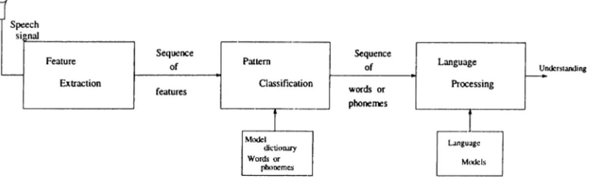
Speech recognition is mainly a pattern classification problem. The general recognition process can be divided into three sub-tasks, feature extraction, pattern classification and language processing, as shown in Figure 1.3.
Figure 1.3: The block diagram of a speech recognition system.
The first step in speech recognition is to extract meaningful features from the speech signal. Feature extraction is usually based on the short-time spectral information of the speech signal. The spectral information is used to be modeled by either linear predictive analysis or Short-Time Fourier Transform (STFT) based features. LP filter derived or Short-Time Fourier Transform (STFT) based
feature sets are used to model the spectral information [7]. In this thesis subband analysis or equivalently wavelet based feature sets are constructed from the speech signal as an alternative to the commonly used Fourier domain feature sets. There are two important sub-tasks that should be done before and after the feature extraction process. Channel adaptation is a front-end process for feature extraction. The end-point detection should be performed by using the extracted features. In this thesis adaptive noise cancelation techniques are developed for channel adaptation, and a new distance measure based on the subband energy levels for the end-point detection is introduced.
The recognizer is first trained by a set of data containing the words in the vocabulary of the system. A dictionary of feature sequences is constructed from the training data corresponding to the words and phonemes in the vocabulary. Then task of pattern classifier is to match the observed sequence of feature sets with the sequences in the dictionary, and to chose the most likely dictionary entry. Hidden Markov Models (HMM), artificial neural-nets, template matching methods based on dynamic programming are the basic pattern classifier methods used in speech recognition. The HMM formalism is the most widely used one among these methods [5]. This statistical approach achieves quite satisfactory recognition rates [7, 22].
The last block of the speech recognition system is the language processing unit. The complexity of the language processing unit is application dependent. For simple applications, such as isolated word recognition, it is only a decision mechanism. For large vocabulary continuous speech recognition systems, it can be a set of rules verifying the grammar of the language [23].
Basic dimensions of the speech recognition problem can be considered as follows
• Degree of speaker independence : The performance of the speaker depen dent recognition systems are superior.
• Size of vocabulary : Large vocabulary increase the error rates.
• Speaking rate and coarticulation : Recognition of isolated words are easier than that of continuous speech.
• Speaker variability and stress : Only for very simple cases, machines can handle these conditions as good as humans.
• Channel conditions : Noise strongly affects the performance of the recogni tion process.
Each of these dimensions should be considered before the planning of the applications, as the robustness of the speech recognizer will be determined according to the above parameters.
In this thesis, the feature extraction problem is considered. Speech feature parameters which are robust to variations in the original speech model assumptions are introduced. The performance of the new feature sets are evaluated using an isolated word recognition system based on an HMM structure. In the following subsection the HMM formalism is briefly reviewed.
1.2.1
H id d en M arkov M o d el (H M M )
The pattern classification block is one of the key elements of a speech recognition system. In this block the speech feature vectors previously extracted from the speech signal vectors are processed. The recognition problem is to associate the sequence of feature vectors a word or a phoneme in the vocabulary.
Starting from the 1970s and mostly in 1980s, researchers working in the field of speech processing concentrated on the modeling of speech signal with stochastic approaches to address the problem of variability. The use of probabilistic modeling brought some advantages over the deterministic approaches. There are mainly two stochastic approaches in the speech recognition research. The first. Hidden Markov Model (HMM), is the stochastic finite state automaton, and the second is the Artificial Neural Networks (ANN). In this subsection the overview of the HMM formalism is given, since the HMM formalism is used as the pattern classifier in this thesis.
The HMM was first introduced to speech recognition field with the independent works of Baker at Carnegie-Melon University (1975) and Jelinek at IBM (1975). The HMM became popular in the last two decades and formed
the basis of many successful, large-scale speech recognition systems.
The HMM is a stochastic finite state automaton that is used to model the speech utterances such as word or subwords. In the HMM formalism the speech utterance is first reduced to a sequence of features. These speech features are also called observations,
{!/(l),!/(2),...,!,(r)} (1.28) where y(i) is the feature vector corresponding to the z-th speech frame and T is the total number of frames in the speech utterance. Entries of the vector, y(i), may be the reflection coefRcients, the LSF’s or the new parameters described in Chapter 2-4 in this thesis. In this formalism, it is assumed that this sequence of observations is generated by a “hidden” finite state automaton. The classification problem is to determine the finite state automaton which produces the current observation sequence with the highest likelihood. It is important to note that every word or subword in the vocabulary is uniquely associated with an HMM, and in order to obtain a reliable speech recognition system the HMM’s corresponding to the words in the vocabulary should be trained over a large population.
a(4l4)
F’igure 1.4: Left to right HMM model.
Although the finite state automaton can be in any configuration, in speech recognition usually the left-to-right model is used. The structure of a typical left-to-right HMM with four states is shown in Figure 1.4. The HMM can be characterized by a two stage probabilistic process. The first one is the allowable state transitions which are occured in the model at each observation time. The
likelihoods of these transitions are stated as the state transition probabilities, where a(i |i) is defined as the transition probability from state j to i as follows:
a (i|i) = P{x{t) = i\x{t - 1 ) = j ) (1.29) where x{t) is the state at time t. And the state transition matrix is given by
a ( l|l) a(l|2) «(1|5)
<i(5|l) a(S|2) ■·■ <i(5|5)
(1.30)
where S is the total number of states in the model. An important property of this matrix is = 1· That is, the entries of columns sum to 1 since, a ( / |j ) ’s are probabilities. The state transition probabilities are assumed to be stationary in time, that is a ( i|j) ’s do not depend upon the time t. Due to this the random sequence is called a first order Markov process.
The second stage of the stochastic process is the generation of observations in each state. An observation probability density function /y|£(f)(ClO is assigned to each state i. Therefore the occurrence of the observations is governed by the pdf of each state. For the completeness of the HMM formalism, the state probability vector at time t is defined as follows,
n(() = P i r n = 1) P (x(i) = 2) P{x(t) = S) 1) and U{t) = A‘- 'n ( l ) .
In summary an HMM, A, is characterized by the following parameters
A = { 5 . I I ( l ) , / l , { 4 | , ( C | i ) , l < i < 5 } }
(1.31)
(1.32)
(1.33)
where S is the total number of states in the model, 11(1) is the initial state probability matrix, A is the state transition matrix, and /y|x’s are the observation probability density functions.
HM M Problem s:
As indicated before, two key problems appear. These are the training and recognition problems.
The Training Problem:
Given a series of training observations for a given word, how do we construct an HMM for this word?
The Recognition Problem:
Given the trained HMM’s for each word in the vocabulary, how do we find the HMM which produces the current observation sequence with the highest likelihood?
These questions will be examined in the following subsections.
T he D iscrete O bservation HMM;
A multidimensional observation probability density function is associated with each state of the finite state automaton. When a particular state is reached an observation vector is generated according to this multidimensional pdf. The HMM is called the discrete (continuous) observation HMM when the observation pdf is a discrete (continuous) pdf. The discrete pdf’s are usually constructed using vector quantization methods.
Let the observation pdf generate K distinct vectors for state i. In other words, the observation pdf for state i reduces to the form of K impulses on the real line for the discrete observation HMM. These observation probabilities are defined as.
6(^|г) = Pi yi t ) = ¿|x(i) = г), k =
and the observation probability matrix is formed as.
(1.35)
B =
6(1|1) 6(1|2) 6(115)
6(i:|i) 6(/i|2) ·■■ 6(A-|5)
In the case of discrete observation HMM, the model, A, can be modified as, A = { 5 ,n (l),A ,5 ,{ t/fc ,l < k < K ] ] (1.37) where {?/*:,] ^ k < K } represents the K possible observation vectors or equivalently the VQ codebook constructed in the training phase.
R ecognition
Given the fully trained HMMs for each word in the vocabulary and the quantized observation sequence (?/(l), j/(2) , ..., ?/(r)}, it is tried to find the likelihood that each model could have produced the observation sequence in the recognition phase.
The partial observation sequences are defined for simplicity of the analysis as follows.
y\ = {i^(l),y(2) r - - , y (0 }
i^i+i = {y{t + l),y{t + 2),· ·· ,y{ r) }
(1.38) (1.39) where y{ and yf^^ are called as forward and backward partial sequences of observations, respectively.
Forward-Backward (F-B) Approach:
An efficient way of computing the likelihood, P(y\A), is the so-called forward- backward (F-B) algorithm of Baum et.al. [24]. It is necessary to define a forward going and a backward-going probability sequence for this method. The joint probability of having generated the partial forward sequence y[ and having arrived at state i at time t, given HMM A, is defined aa.
" (2/1 , 0 = P{y!-i = y{,x{t) = i|A). (1.40) Similarly, the probability of generating the backward partial sequence yj^_^ is defined as,
= Pia.1, = S.+iWO = ‘.A)· (!■«) Although, we only need the ex sequence to compute the /^(j/jA), we define /3 sequence for a future use in the training algorithm.
Suppose we are at time t + 1 and wish to compute for some state
j. We should add up all the probabilities for all of the possible paths to state j
at i + 1, that arising from all of the possible states at t. Then, clearly
+ 1) = i)P{y{t + 1) = y{t + l)|x (i + 1) = j )
1=1
5
= W ) · (1-42)
t=l
Hence, the ot sequence can be computed with a lattice type structure and the recursion is initiated by setting.
= -PU(l) = i)i>(2/(l)li)
1 < i < 5.
Similarly, the backward recursion can be derived for the /3 sequence:
^(yS-ilO = S^(2/i+2»Oa(iN)%(^+ l)li)
i=i where the recursion is initiated as,
^(i/T+ilO =
Now, it is clear that.
1 if i is a legal final state
0 else
Piy,x{t) = i|A) = a{yl,i)/3{yl^^\i)
for any state i. Therefore,
P{y\^) = Z ;« (i/i>0^ (2/t+il0 ·
t=l
Also, we can express the likelihood as,
p ( y \ ^ ) = L ! oc{yj,i).
all legal final i
(1.43) (1.44) (1.45) (1.46) (1.47) (1.48)
Training
Training a particular HMM to correctly represent its designated word is equivalent to finding the appropriate model matrices A and B, and the initial state probability vector 11(1). The F-B algorithm provides an iterative estimation procedure for computing a model, A.
Let us define some new sequences to build up the estimation procedure,
= P{u{t) = Uj\,\y,A)
= P (u(i) = u,|,,i/|A)/P(2/|A)
P{y\A) , U-4Jj
where u{t) represents the transition at time i, Uj|¿ is the transition from state i to j and ^ is the probability of making a transition from state i to state j at time
= P{u{t) eu.\i\y,A)
i=l
0‘(y\A)/3{yI+i\j) K t < c T - l
p { y m ‘
where u.^i is the set of transitions exiting state i and 7 is the total probabilit}^ of making transitions from state i to all other states at time
= j \y ^ ^ )
7( i; 0 i < i < T - i
t = T
0‘{y\J)l^{yI+i\j) K t < T
P{y\^)
where v is the probability of being at state j at time t,
6U, k-t ) = P{y^{t) = k\y,A)
u{j\ t) if y{t) = k and 1 < t < T 0
(1.51)
where y_j{t) models the observation being emmited at state j and at time t, and
6 is the probability of observing A;-th observation vector at state j and at time t.
From these sequences four related key results can be computed: T - J
(1.53) t = l
where ·) is the total probability of making a transition from state i to state T - l
7 (11 ■) = P{u{·) e A ) = Y ^ lit; i) (1.54)
i = \
where 7(z; ·) is the total probability of making a transition from state i to all possible states,
>'(};■) = r i u i · ) € tij|.|!/,A) = (1.55)
i=l
where u{j\ ·) is the total probability of making a transition from all possible states to state j, and
= P ( i y ) i ( · ) = ' ’ I f ' ' ' ) = (1.56)
i=l
where ¿{j, k] ·) is the total probability of observing the A:-th observation while making a transition to state j.
With these interpretations, the following reestimation equations can be written, a(ilO = b(k\j) = P{x{l) = г) = 7(*; ·) (^{yl,i)a{j\i)b{y{t + l)\j)^{yj^2\j) ·) i:i=,Mt)=k^iyUMyI+i\j) E L · o/{y\J)^{yI+i\j) t(*; 1) P(y\^) ■ (1.57) (1.58) (1.59)
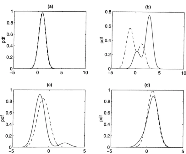
(a)
(b)(c)
(d)Figure 1.5: Observation probability densities of digit zero (line), and four (dotted) for states (a) one, (b) two, (c) three, and (d) four.
The Continuous Observation HMM:
In the more general case in which the observations are continuous, the distributions of observations within each state characterized by a multivariate pdf. In the recognition problem, the likelihood of generating observation y{t) in state j is simply defined as
% ( 0 li) = 4ix(i/(0l;)·
(1.60)The most widely used form of observation pdf is the Gaussian mixture density, which is of the form
M
I
771 = 1
where Cim is the mixture coefficient for the m-th component for state and Ai{·) denotes a multivariate Gaussian pdf with mean pim and covariance matrix Cim· With this formulation the training problem can be solved with simple reestimation procedures [25]. A detailed description of the training problem can be found in [5, 22].
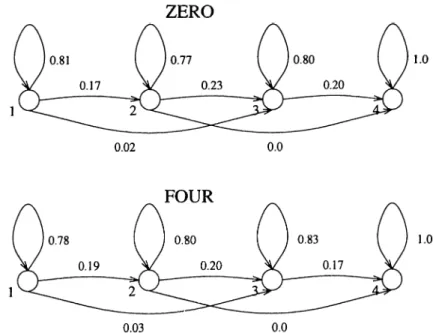
An illustrative example for the observation probability densities of a four- state HMM structure with 3 mixture densities are given in F'igure 1.5. These observation densities correspond to the fourth element of the observation vector for two English digits zero and four. The state transition probabilities for these digits are given in Figure 1.6.
ZERO
1.0
1.0
Figure 1.6: HMM structures for English digits zero and four.
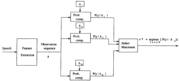
In the isolated word recognition systems the elements of the vocabulary are discrete words. Consider a recognition system with a F-word vocabulary. First, for each word in the vocabulary an HMM model, A„ 1 < u < F , is built using the training data as described in subsection 1.2.1. A graphical description of this procedure is depicted in Figure 1.7. During the recognition process the observation sequence y = ?/(l), y(2), · · ·. j/(T) is extracted from the speech signal, and the probabilities P(y|A,,) a.re evaluated for each word. The result
is determined according to the HMM word model which produces the highest likelihood [5].
Figure 1.7: HMM recognizer.
The elements of the vocabulary may be phonemes as well. In many large vocabulary continuous speech recognition systems the continuous speech signal is first segmented into phonemes. Then the current phoneme is determined over the vocabulary containing all possible phonemes. Both in English and Turkish, the spoken language can be represented by about 40 phonemes. Given a good phoneme segmentation method, an HMM based recognition system can easily handle 40 phonemes when the speech is noise-free.
1.3
S p eech R eco g n itio n R esearch in T urkey
During the last 10 years several researchers have developed speech recognition systems for Turkish. All of these systems consider isolated word recognition and vowel recognition [26, 27, 28, 29, 30]. These systems are described in a speech workshop that was held in Middle East Technical University (METU) on May 1995 [31]. The studies in Hacettepe University cover the isolated word recognition systems based on discrete density HMM structures with LP deri^·ed cepstral
features [31]. Isolated word and vowel recognition systems based on dynamic time warping and artificial neural networks are also investigated in Osmangazi University [27, 30, 31].
We recently finished voice dialing project for mobile telephones in cooperation with TÜBİTAK-BİLTEN [26, 31]. This project was also supported by ASELSAN, and some of the techniques developed in this thesis are successfully used in this project. The Turkish speech databases collected for this project are used in the simulation studies in Chapter 2 and Chapter 3.
One of the important result of the METU speech workshop was the lack of a speech corpus for Turkish speech recognition studies. In this workshop the need to construct a national speech corpus which is extremely important for speech recognition research was pointed out and TUBITAK-BILTEN will prepare a speech corpus. Besides this, Hacettepe University, and Osmangazi University have their own recordings that include the isolated Turkish digits and some control words.
LINE SPE C T R A L
FR E Q U E N C IE S IN SP E E C H
R E C O G N IT IO N
As indicated in Chapter 1, extraction of feature parameters from the speech signal is the first step in speech recognition. The feature parameters are desired to have perceptually meaningful parameterization and yet robust to variations in environmental noise. In this chapter, a new set of speech feature parameters based on the Line Spectral Frequency (LSF) representation in subbands, SUBLSF's, is introduced.
The LSF representation of speech is reviewed in Section 2.1. The new speech feature parameters, SUBLSFs are described in Section 2.2. The parameters are used in a speaker independent continuous density Hidden Markov Model (HMM) based isolated word recognition system operating in the presence of car noise. The simulation results are described in Section 2.2.1.
2.1
LSF R ep resen ta tio n o f Speech
Linear ¡predictive modeling techniques are widely used in various speech coding, synthesis and recognition applications. The Line Spectral Frequency (LSF) representation of the linear prediction (LP) filter is introduced by Itakura [18]. LSFs are closely related to formant frequencies and they have some desirable properties which make them attractive to represent the Linear Predictive Coding (LPC) filter. The quantization properties of the LSF representation is recently investigated in [19, 20, 32].
Let the m -th order inverse filter Am(z),
Am{^) — 1 + dlZ ^ + · · · + UmZ (2.1)
be obtained by the LP analysis of speech. As defined in Section 1.1.2, the LSF polynomials of order (m + 1), Pm+i{z) and Qm+\{z)^ are constructed by setting the (m + l)-s t reflection coefficient to 1 or —1. In other words, the polynomials,
Pm^i{z) and Qm+i(z), are defined as.
and
P^+^(z} = Am{z) + z-^”^+^^A^{z-%
Q„,+ l{z) = A^{z) - Z-^^+^Umiz-^).
(2.2)
(2.3) The zeros of Pm+\{z) and Qm+i{z) are called the Line Spectral Frequencies (LSFs), and they uniquely characterize the LPC inverse filter Am{z and
Qm+i{z) are symmetric and anti-symmetric polynomials, respectively. Therefore,
it is possible to decompose the power spectrum |Am(i^)P as
(2.4) Roots of the LP polynomial corresponds to the peaks or the formants of the spectra of the speech signal. By examining Equation (2.4) it can be seen that the roots of Am{z) (or the formants) are related with the roots of the Pm+\iz) and
Qm+-i{z)· In order to illustrate this relationship between formants and the LSFs
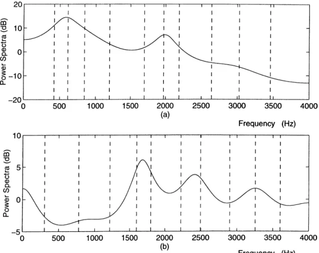
more clearly, the LP spectrum and the associated LSFs are plotted in Figure
that the cluster of (two to three) LSFs characterizes a formant frequency and the bandwidth of a given formant depends on the closeness of the corresponding LSFs. In addition, the spectral sensitivities of LSFs are localized. That is, a change in a given LSF produces a change in the LP power spectrum only in its neighborhood.
Frequency (Hz)
Figure 2.1: LP power spectrum and the associated LSFs for (a) vowel / a / and (b) fricative /s h /.
2.2
LSF R ep resen ta tio n in Subbands for S p eech
R ecogn ition
In this section, a new set of speech feature parameters is constructed from subband analysis based Line Spectral Frequencies (LSFs) [33]. The speech signal is divided into several subbands and the resulting subsignals are represented by LSFs. The performance of the new speech feature parameters, SUBLSFs, is compared with the widely used Mel Scale Cepstral CoefTicients (MELCEPs). SUBLSFs are observed to be more robust than the MELCEPs in the presence of car noise.
It is well known that LSF representation and cepstral coefficient represen tation of speech signals have comparable performances for a general speech recognition system [34, 35]. Car noise environments, however, have low-pass characteristics which may degrade the performance of a general full-band LSF or mel scaled cepstral coefficient (MELCEP) representations [5]. In this section, LSF based representation of speech signals in subbands is introduced.
The speech signal is filtered by a low-pass and a high-pass filter and the LP analysis is performed on the resulting two subsignals. Next, the LSFs of the subsignals are computed and the feature vector is constructed from these LSFs. More emphasis to the high-frequency band is given by extracting more LSFs from the high-band than the low-frequency band.
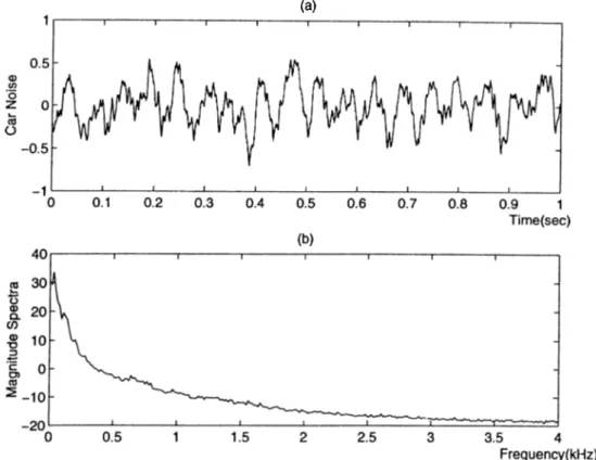
The mel scale is accepted as a transformation of the frequency scale to a perceptually meaningful scale, and it is widely used in feature extraction [36]. However the environmental noise may effect the performance of the mel scale derived features. It is experimentally observed that significant amount of the spectral power of car noise^ is localized under 500 Hz. Figure 2 .2 shows an utterance from the Volvo 340 recording, and the average spectra of this recording. Due to this reason the LP analysis of speech signal is performed in two bands, a low-band (0-700 Hz) and a high-band (700-4000 Hz). In this case the high-band can be assumed to be noise-free.
'This noise is recorded inside a Volvo 340 on a rainy asphalt road by In stitu te f o r P e r c e p t io n - T N O . T h e N eth erlan ds.
This kind of frequency domain decomposition can be generalized to cases in which the noise is frequency localized.
(a)
Figure 2.2: (a) Car noise time series, (b) Car noise spectra for Volvo 340 recording.
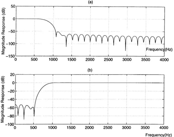
In simulation studies a continuous density Hidden Markov Model (HMM) based speech recognition system is used with 5 states and 3 mixture densities. Simulation studies are performed on the vocabulary of ten Turkish digits (Oisifir, l:bir, 2:iki, 3:ug, 4:dort, 5:be§, 6:alti, 7:yedi, 8:sekiz, 9:dokuz) from the utterances of 51 male and 51 female speakers. The isolated word recognition system is trained with 25 male and 25 female speakers, and the performance evaluation is done with the remaining 26 male and 26 female speakers. The speech signal is sampled at 8 kHz and the car noise is assumed to be additive. The low-pass and high-pass filters are chosen as 5Tth order linear phase FIR filters. The magnitude responses of the low-pass and the high-pass filters are shown in Figure 2.3(a) and
Figure 2.3(b), respectively.
(a)
Figure 2.3: Magnitude responses of the (a) low-pass and the (b) high-pass filters.
2.2.1
P erform an ce o f LSF R ep re sen ta tio n in Subbands
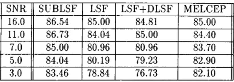
Both 12-th and 2 0-th order LP analyses are performed on every 10 msec with a window size of 30 msec (using a Hamming window) for low-band (noisy band) and high-band (noise free band) of the speech signal, respectively. The first 5 LSFs of the low-band and the last 19 LSFs of the high-band are combined to form the Subband derived LSF feature vector (SUBLSF). The recognition rate of SUBLSFs are recorded in Table 1 under various SNRs.
feature sets. The recognition rates of four feature sets, SUBLSF, LSF, LSF-fDLSF, and MELCEP, for various SNR values are also given in Table 2.1.
Table 2.1: Recognition rates of SUBLSF, MELCEP and LSF representations in percentage. SNR 16.0 11.0 7.0 5.0 3.0 SUBLSF 86.54 86.73 85.00 84.04 83.46 LSF 85.00 84.04 80.96 80.19 78.84 LSF+DLSF 84.81 85.00 80.96 79.23 76.73 MELCEP 85.00 84.40 83.70 82.90 82.10
In column 2 of Table 1 the full-band LSF representation is investigated. The size of the LSF vector is 24 which is obtained by a 24-th order LP analysis. The recognition rate of LSFs with their time derivatives, DLSFs, is also obtained. In this case 1 2-th order LP analysis is carried out to construct the 24-th order DLSF feature vector. The results are summarized in column 3 of Table 1.
In column 4 the results of MELCEP representation is given. Frequency domain cepstral analysis is performed to extract 1 2 me/ scale cepstral coefficients and a 24-th order MELCEP feature vector is obtained from 1 2 me/-scale cepstral coefficients and their time derivatives.
In our simulation studies we observed that the SUBLSFs have the highest recognition rate.
2 .2 .2
C on clu sion
In this chapter, a new set of speech feature parameters based on LSF representation in subbands, SUBLSFs, is introduced. It is experimentally observed that the SUBLSF representation provides higher recognition rate than the commonly used MELCEP, LSF, LSF+DLSF representations for speaker independent isolated word recognition in the presence of car noise. Since the car noise is concentrated in low frequencies, the high frequency bands can be
assumed to be noise free. This property is exploited in this chapter to achieve robustness against noise.
The computational compIexiW the SUBLSF scheme is clearly higher than the LSF and cepstral analysis methods, because two LP analyses are carried out in two subbands. In the next chapter a computationally efficient method for feature parameter extraction is introduced. The method is also based on subband analysis.
W AVELET A N A LY SIS FO R
SPE E C H R E C O G N IT IO N
In this chapter, a new set of feature parameters for speech recognition is presented. The new feature set is obtained from the root-cepstral coefficients derived from the wavelet analysis of the speech signal [37]. The performance of the new feature representation is compared to the mel scale cepstral representation (MELCEP) in the presence of car noise. Subband analysis based parameters are observed to be more robust than the commonly employed MELCEP representation.
The first step in automatic speech recognition is the extraction of acoustic features which characterize the speech signal in a perceptually meaningful manner. Many feature parameter sets including Linear Predictive Coding (LPC) parameters, Line Spectral Frequencies (LSF’s), and cepstral parameters were used for speech recognition in the past [2 2, 34, 35, 38]. Among these methods the ones based on cepstral analysis are the most widely used in applications where noise is present [39]. This is due to the compatibility of some cepstral methods with the human auditory system. The new parameters are based on wavelet analysis or equivalently the multirate subband analysis which provides robust recognition performance by appropriately deemphasizing frequency bands that are corrupted by noise.
The new feature parameters are obtained via a two stage procedure. First, the frequency domain is partitioned into nonuniform regions using a basic half band filter bank in a tree structured manner. As a result a family of subband signals are obtained. In order to incorporate the properties of the human auditory perceptual system the frequency range lower than IkHz is uniformly divided whereas a logarithmic partition is applied above 1 kHz. The resulting frequency bands are very similar to the commonly used mel-scale division [36]. After this step, a set of cepstral-like parameters are obtained from the subband signals. This procedure is described in detail in Section 3.1.
The performance of the new Subband based Cepstral parameters, SUBCEPs, is tested in the presence of car noise. The SUBCEPs are compared to the short-time Fourier Analysis based methods. The SUBCEP parameters are observed to produce better recognition rates than other currently employed feature parameters. Simulation examples are presented in Section 3.2.
3.1
Subband A n alysis based C ep stral C oefficien t
(S U B C E P ) R ep resen ta tio n
It is well known that the Fourier transform provides information about the frequency content of the signal, but it does not provide any temporal information due to the infinite extent of the Fourier basis functions. Therefore, in many applications including speech processing the short-time Fourier analysis is performed with overlapping time windows to obtain temporal information. On the other hand the wavelet transform is ideally suited for the analysis of signals with time varying characteristics. The new speech feature parameters described in this section are derived from the wavelet transform coefficients.
The wavelet analysis associated with a subband decomposition filter bank provides a fast and computationally efficient structure for decomposing the frequency domain along with the temporal information. The basic building block of a wavelet transform which is a multirate signal processing techniq\ie is realized by a subband decomposition filter bank as shown in Figure 3.1. The
filter bank structure consists of a lowpass and a highpass filter, and downsampling units. The passbands of the low and high pass filters are [0, tt/2] and [7t/2. tt],
respectively, so that the frequency domain is divided into two halfbands. In the subband decomposition filter bank structure the input signal is first filtered by the complementary low-pass and high-pass filters and then the outputs of the filters are passed to the downsampling units which drop every other sample of their inputs reducing the sampling rate by a factor of two. In this way two tem poral subsignals containing the low and high frequency components of the original signal are obtained. The simple filter bank structure of Figure 3.1 provides a time-frequency decomposition of the original signal with the frequency regions, [0, Tr/2] and [7t/2, 7t]. Each of the subsignals can be further decomposed into two new subsignals using the same filter bank once again, and this analysis procedure can be repeated until the desired frequency domain decomposition is obtained. Resulting temporal subsignals constitute the so-called wavepacket representation uniquely characterizing the original signal [40]. The original signal in turn can be perfectly reconstructed (or synthesized) from the subsignals, if the lowpass and highpass filters are properly selected [40, 41].
Figure 3.1: Basic block of subband decomposition.
In this work, a subband decomposition filter bank corresponding to a biorthogonal wavelet transform [41, 42] is used in simulation studies. The low- pass filter, Ho(z), and the high-pass filter, for this filter bank have the form
(3.1) 1