Optical implementations of two-dimensional fractional Fourier transforms and linear canonical transforms with arbitrary parameters

(1)

Optical implementations of two-dimensional fractional

Fourier transforms and linear canonical transforms

with arbitrary parameters

Aysegul Sahin, Haldun M. Ozaktas, and David Mendlovic

We provide a general treatment of optical two-dimensional fractional Fourier transforming systems. We not only allow the fractional Fourier transform orders to be specified independently for the two dimen-sions but also allow the input and output scale parameters and the residual spherical phase factors to be controlled. We further discuss systems that do not allow all these parameters to be controlled at the same time but are simpler and employ a fewer number of lenses. The variety of systems discussed and the design equations provided should be useful in practical applications for which an optical fractional Fourier transforming stage is to be employed. © 1998 Optical Society of America

OCIS code: 070.2590.

1. Introduction

The fractional Fourier transform has received consid-erable attention since 1993.1–13 _Several

applica-tions of the fractional Fourier transform have been suggested. In particular, many signal- and image-processing applications have been developed on the basis of the fractional Fourier transform.14 –25

Sev-eral two-dimensional ~2-D! optical implementations have been discussed previously,1,4,6,8,11,26 –28 _{but a}

comprehensive and systematic treatment did not ex-ist until Ref. 29, in which we provided a detailed examination of the 2-D fractional Fourier transform. In this paper we provide a very general treatment of optical 2-D fractional Fourier transforming systems. We allow the fractional Fourier transform orders to be specified independently for the two dimensions. We also allow the input and output scale parameters and the residual spherical phase factors to be controlled. We further discuss systems that do not allow all of these parameters to be controlled at the same time but are simpler and employ a fewer number of lenses.

We begin by reviewing the properties of the 2-D fractional Fourier transform. Some of these are trivial extensions of the corresponding one-dimensional ~1-D! property or have been discussed elsewhere, although they do not appear collectively in any single source. For this reason we list them with minimum comment.

In Section 3 we present optical realizations of linear canonical transforms. Since linear canonical trans-forms can be interpreted as scaled fractional Fourier transforms with additional phase terms, these systems can realize fractional Fourier transforms with desired orders, scale factors, and residual phase terms. In Section 4 we consecutively consider systems with two, four, and six cylindrical lenses. In each case we dis-cuss which parameters it is possible to specify inde-pendently and which parameters we have no control over. One can choose from among these systems the one that provides the required flexibility with the min-imum number of lenses.

2. Two-Dimensional Fractional Fourier Transform The 2-D fractional Fourier transform with the orders

axfor the x axis and ayfor the y axis, for 0, uaxu , 2

and 0, uayu , 2, respectively, is defined as

^ax,ay@ f~x, y!#~x, y! 5

*

2` `

*

2` ` Bax,ay~x, y; x9, y9! 3 f~x9, y9!dx9dy9, (1)

When this research was performed, A. Sahin and H. M. Ozaktas were with the Department of Electrical Engineering, Bilkent Uni-versity, TR-06533 Bilkent, Ankara, Turkey; D. Mendlovic was with the Faculty of Engineering, Tel-Aviv University, 69978 Tel-Aviv, Israel. A. Sahin is now with the Department of Economics, Uni-versity of Rochester, Rochester, New York 14627.

Received 17 June 1997; revised manuscript received 4 December 1997.

(2)

where

Bax,ay~x, y; x9, y9! 5 Bax~x, x9!Bay~y, y9!, (2)

Bax~x, x9! 5 Afxexp@ip~x 2_cot_f x 2 2xx9 csc fx1 x9 2 cotfx!#, (3)

Bay~y, y9! 5 Afyexp@ip~y

2_cot_f

y

2 2yy9 csc fy1 y92cotfy!#, (4)

A_f_x5exp@2i~pfˆxy4 2 fxy2!#

~usin fxu!1y2

,

A_f_y5exp@2i~pfˆyy4 2 fyy2!#

~usin fyu!1y2

, (5)

fx 5 axpy2, fy 5 aypy2, fˆx 5 sgn~fx!, and fˆy 5

sgn~fy!. As Eq. ~2! suggests, the kernel Bax,ay is a

separable kernel.

The definition may be simplified by use of vector-matrix notation: ^@ f~r!#~r! 5

*

2` ` A_f_rexp@ip~rTCtr2 2r T Csr* 1 r*T Ctr*!#f~r*!dr*, (6) where A_f_r5 A_f_xA_f_y, r5 @x y#T_, _r_{* 5 @x9 y9#}T_, Ct5

F

cotfx 0 0 cotfy

G

, Cs5

F

cscfx 0 0 cscfy

G

. Two-~and higher-! dimensional30_{fractional Fourier}

transforms were first considered with equal orders

ax5 ay, and their optical implementations involved

spherical lenses and graded-index media~see the ref-erences in the first paragraph of Section 1!. The possibility of different orders was mentioned in Ref. 4 and discussed in Refs. 26 –28.

A. Properties of Two-Dimensional Fractional Fourier Transforms

Most of the following properties are straightforward generalizations of the 1-D versions.31–33

1. Additivity

^ax1,ay1^ax2,ay2_f~x, y! 5 ^ax11ax2,ay11ay2_f~x, y!. ₍₇₎

2. Linearity

For arbitrary constants ckwe find

^ax,ay

(

k ckf~x, y! 5

(

k ck^ax,ayf~x, y!. (8) 3. Separability If f~x, y! 5 f~x! f~y!, then ^ax,ay_f~x, y! 5 @^ax_f~x!#@^ay_f~y!#. ₍₉₎ 4. Inverse Transform Bax,ay 21_{~x, y; x9, y9! 5 B} 2ax,2ay~x, y; x9, y9!. (10) 5. Unitarity

The 2-D kernel is unitary, as shown by

Bax,ay

21_{~x9, y9; x, y! 5 B}

2ax,2ay~x9, y9; x, y! 5 B*ax,ay~x, y; x9, y9!, (11)

where the asterisk denotes the complex conjugate.

6. Parseval Relation

*

2` `

*

2` ` f~r*!*g~r*!dr* 5

*

2` `

*

2` ` $^ax,ay_f~r*!%* 3 $^ax,ay_g~r*!%dr*, ₍₁₂₎

*

2` `

*

2` ` uf~r*!u2 dr* 5

*

2` `

*

2` ` u^ax,ay_f~r*!u2_dr*. (13)

7. Effect of the Coordinate Shift

The fractional Fourier transform of f~x 2 x₀, y2 y₀! can be expressed in terms of the fractional Fourier transform of f~x, y! as ^ax,ay@ f~r 2 r 0!#~r! 5 exp

H

2i2p

F

rs T

S

r21 2rc

DGJ

3 ^ax,ay@ f~r!#~r 2 r c!, (14) where r05 @x0 y0#T, rc5 @x0cosfx y0cosfy#T, rs5 @x0sinfx y0sinfy#T.

8. Effect of Multiplication by a Complex Exponential

If a function f~x, y! is multiplied by an exponential exp@i2p~mxx1 myy!#, the resulting fractional Fourier

transform becomes ^ax,ay@exp~i2pmT_r! f~r!# 5 exp$ip@m cT~ms1 2r!#% 3 ^ax,ay@ f~r!#~r 2 m s!, (15) where m5 @mx my# T , c5 @mxcosfx mycosfy# T , ms5 @mxsinfx mysinfy#T.

(3)

9. Multiplication by Powers of the Coordinate Variables

The fractional Fourier transform of xm_yn_f_{~x, y! for m,}

n$ 0 is ^ax,ay@xm_yn_f~x, y!# 5

S

_{x cos}f x1 i psinfx ] ]x

D

m 3

S

y cosfy1 i psinfy ] ]y

D

n 3 ^ax,ay_f~x, y!. ₍₁₆₎ 10. Derivative of f~x, y!

The fractional Fourier transform of the term ~]m_y]m_x_!~]n_y]n_y_{! f~x, y! is} ^ax,ay

F

] m ]xm ]n ]ynf~x, y!

G

5

S

i2px sin fx1 cos fx ] ]x

D

m 3

S

i2py sin fy1 cos fy ] ]y

D

n 3 ^ax,ay_f~x, y!. ₍₁₇₎ 11. Scaling

The fractional Fourier transform of f~k_xx, k_yy! can be

represented in terms of the fractional Fourier trans-form of f~x, y! with different orders a_x9 and a_y9 as

^ax,ay@ f~Kr!#~r! 5 C exp~iprT_Dr!^ax9,ay9@ f~r!#~K*r!, (18) where C5 AfxAfy ukxuukyuAfx9Afy9 , K5

F

kx 0 0 ky

G

, fx9 5 arctan~kx2tanfx!, ax9 5 2a_f_x₉ p , fy9 5 arctan~ky2tanfy!, ay9 5 2a_f_y₉ p , D5

3

cotfx kx42 1 kx41 cot2fx 0 0 cotfy ky42 1 ky 4 1 cot2 fy

4

, K* 5

3

sinfx9 kxsinfx 0 0 sinfy9 kysinfy

4

. 12. Rotation Let R5

F

cosu sinu 2sin u cos u

G

;

then f~Rr! 5 f~cos ux 1 sin uy, 2sin ux 1 cos uy! represents the rotated function with the angle u. When it is the case that a_x5 a_y5 a, then

^a

@ f~Rr!#~r! 5 ^a

~r!~Rr!. (19)

13. Wigner Distribution and Fractional Fourier Transform

Let W_f~x, y; n_x,n_y! be the Wigner distribution of f~x, y!. If g~x, y! is the fractional Fourier transform of f~x, y!, then the Wigner distribution of g~x, y! is related to that of f~x, y! through the following:

Wg~r, n! 5 Wf~Ar 1 Bn, Cr 1 Dn!, (20) where r5 @x y#T_, _{n 5 @n} x ny#T, (21) A5

F

cosfx 0 0 cosfy

G

, B5

F

2sin fx 0 0 2sin fy

G

, (22) C5

F

sinfx 0 0 sinfy

G

, D5

F

cosfx 0 0 cosfy

G

. (23) As Eq.~20! suggests, the effect of the fractional Fou-rier transform on the Wigner distribution is a coun-terclockwise rotation with the angle fx in the x–nx

plane and the anglefyin the y–nyplane.

14. Projection

The projection property of a 1-D kernel34_{states that}

the projection of the Wigner distribution function on an axis making an angle f with the x axis is the absolute square of the fractional Fourier transform of the function with the order a~f 5 apy2!. This effect can be represented in terms of the Radon transform as

5f@W~x, n!# 5 u^a@ f~x!#u2, (24)

where the Radon transform of a 2-D function is its projection on an axis making an anglef with the x axis. The separability of the 2-D kernel can be used to derive the corresponding property for the 2-D case. If the Radon transform is applied successively to the Wigner distribution W~x, y; nx,ny!, then the property

becomes

5fy$5fx@W~x, y; nx,ny!#% 5 u^

ax,ay@ f~x, y!#u2_. ₍₂₅₎ Thus the projection of the Wigner distribution W~x, y; nx,ny! of any function f~x, y! on the plane determined

by two lines—the first making an anglef_xwith the x axis and the second making an anglefy with the y

axis—is the absolute square of its 2-D fractional Fou-rier transform with the orders axand ay.

(4)

15. Eigenvalues and Eigenfunctions

Two-dimensional Hermite–Gaussian functions are eigenfunctions of the 2-D fractional Fourier trans-form:

*

2` `

*

2` ` Bax, ay~x, y; x9, y9!Cnm~x, y9!dx9dy9 5 lnmCnm~x, y!, (26) where Cnm~x, y! 5 21y2 ~2n₂m_n!m!_!1y2Hn~

Î

2px!Hm~

Î

2py! 3 exp@2p~x2_{1 y}2_!#, ₍₂₇₎

lnm5 exp~2ipaxny2!exp~2ipaymy2!. (28)

B. Linear Canonical Transforms and Fractional Fourier Transforms

Fractional Fourier transforms, Fresnel transforms, chirp multiplication, and scaling operations are used widely in optics to analyze systems composed of sec-tions of free space and thin lenses. These linear integral transforms belong to the class of linear ca-nonical transforms. The definition for a 2-D linear canonical transform is g~x, y! 5

*

2` `

*

2` ` h~x, y; x9, y9! f~x9, y9!dx9dy9, h~x, y; x9, y9! 5 exp~2ipy4!bx1y2

3 exp@ip~axx22 2bxxx9 1 gxx92!#

3 exp~2ipy4!by1y2exp@ip~ayy2

2 2byyy9 1 gyy92!#, (29)

where ax, bx, gx and ay, by, gy are real constants.

Any linear canonical transform is completely speci-fied by its parameters. Alternatively, linear canon-ical transforms can be specified by use of a transformation matrix. The transformation matrix of such a system, as specified by the parametersax,

bx,gxanday,by,gy, is T;

3

Ax 0 Bx 0 0 Ay 0 By Cx 0 Dx 0 0 Cy 0 Dy

4

;

3

gxybx 0 1ybx 0 0 gyyby 0 1yby 2bx1 axgxybx 0 axybx 0 0 2by1 aygyyby 0 ayyby

4

, with AxDx2 BxCx5 1 and AyDy2 ByCy5 1.35,36

Propagation in free space and through thin lenses can also be analyzed as special forms of linear canon-ical transforms. Here both the kernels and the transformation matrices of the optical components

are given. The transformation kernel for free-space propagation of length d is expressed as

hf~x, y, x9, y9! 5 Kfexp

H

ip

F

~x 2 x9!2 ld 1 ~y 2 y9!2 ld

GJ

, (30) and its corresponding transformation matrix is

Tf~d! 5

3

1 0 ld 0 0 1 0 ld 0 0 1 0 0 0 0 1

4

. (31)

Similarly, the kernel for a cylindrical lens with focal length fxalong the x direction is

hxl~x, y, x9, y9! 5 Kxld~x 2 x9!exp~2ipx2ylfx!, (32)

with its transformation matrix given by

Txl~ fx! 5

3

1 0 0 0 0 1 0 0 21 lfx 0 1 0 0 0 0 1

4

, (33)

and the kernel for a cylindrical lens with a focal length fyalong the y direction is

hyl~x, y, x9, y9! 5 Kyld~y 2 y9!exp~2ipy2ylfy!, (34)

with its transformation matrix given by

Tyl~ fy! 5

3

1 0 0 0 0 1 0 0 0 0 1 0 0 21 lfy 0 1

4

. (35)

More general anamorphic lenses may be represented by a kernel of the form

hxyl~x, y, x9, y9! 5 Kxyld~x 2 x9, y 2 y9!

3 exp

F

2ip

S

x 2 lfx 1 y 2 lfy 1 xy lfxy

DG

, (36) with the transformation matrix given by

Txyl~ fy! 5

3

0 1 0 0 0 1 0 0 21 lfx 21 2lfxy 1 0 21 2lfxy 21 lfy 0 1

4

. (37)

The transformation-matrix approach is practical in the analysis of optical systems. First, if several sys-tems are cascaded the overall system matrix can be found by multiplication of the corresponding trans-formation matrices. Second, the transformation matrix corresponds to the ray–matrix in optics.37

(5)

Third, the effect of the system on the Wigner distri-bution of the input function can be expressed in terms of this transformation matrix. This topic is dis-cussed extensively in Refs. 35 and 38 – 41.

We already stated in Section 1 that the fractional Fourier transform belongs to the family of linear ca-nonical transforms. So it is possible to calculate the transformation matrix for the fractional Fourier transform. Before finding the transformation ma-trix we modify the definition of the fractional Fourier transform. In some physical applications it is nec-essary to introduce input and output scale parame-ters. It is possible to modify our definition by inclusion of the scale parameters and also the addi-tional phase factors that can occur at the output:

Bax,ay~x, y; x9, y9! 5 Afxexp~ipx

2_p x!exp

F

ip

S

x2 s22 cotfx 22xx9 s1s2 cscfx1 x92 s1 2cotfx

DG

3 Afyexp~ipy 2_p y!exp

F

ip

S

y2 s22 cotfy 22yy9 s1s2 cscfy1 y92 s12 cotfy

DG

. (38)

In the definition in Eq. ~38!, s1 stands for the input

scale parameter and s2 stands for the output scale

parameter. With the phase factors px, py and the

scaling factors s1, s2 permitted, the transformation

matrix of the fractional Fourier transform can be found as

T;

F

A B

C D

G

, (39)

where

3. Optical Implementation of Linear Canonical Transforms and Fractional Fourier Transforms by Use of Canonical Decompositions

In our optical setups we try to control as many pa-rameters as we can. Following is a list of parame-ters that we want to control:

• Order parameters axand ay: The main

objec-tive of designing optical setups is to control the orders of the fractional Fourier transform. Control of the order parameters is our primary interest.

• Scale parameters s1 and s2: It is desirable to

specify both the input and the output scale parame-ters to provide practical setups.

• Additional phase factors p_xand p_y: In our de-signs we try to obtain px 5 py 5 0 to remove the

additional phase factors at the output plane and ob-serve the fractional Fourier transform on a flat sur-face.

In all the systems we analyze below we clearly indi-cate the parameters specified by the designer, the design parameters, and the uncontrollable outcomes, if any.

A. One-Dimensional Systems

1. Canonical Decomposition Type 1

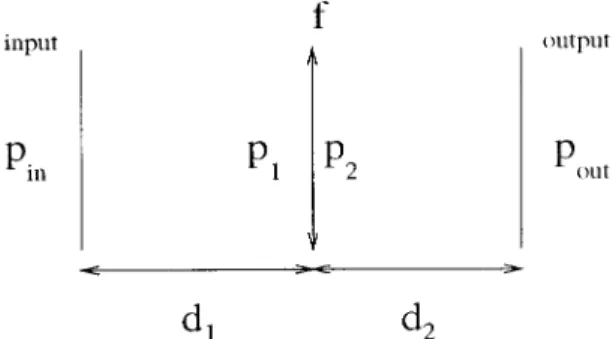
The overall system matrix T of the system shown in Fig. 1 is

T5 Tf~d2!Txl~ f !Tf~d1!. (44)

Both the optical system depicted in Fig. 1 and the linear canonical transform have three parameters. Thus it is possible for one to find the system param-eters uniquely by solving Eq.~44!. The equations for

A5

3

s2 s1 cosfx 0 0 s2 s1 cosfy

4

, (40) B5

F

s1s2sinfx 0 0 s1s2sinfy

G

, (41) C5

3

1 s1s2 ~pxcosfx2 sin fx! 0 0 1 s1s2 ~pycosfy2 sin fy!

4

, (42) D5

3

s1 s2 sinfx~px1 cot fx! 0 0 s1 s2 sinfy~py1 cot fy!

4

. (43)

(6)

d₁, d₂, and f in terms ofa, b, and g are found as d15 b 2 a l~b2_{2 ga!}, d25 b 2 g l~b2_{2 ga!}, f5 b l~b2_{2 ga!}. (45)

Since the fractional Fourier transform is a special form of linear canonical transforms, it is possible to implement a 1-D fractional Fourier transform of the desired order by use of this optical setup. The scale parameters s1and s2can be specified by the designer,

and the additional phase factors px and py can be

made equal to zero. Lettinga 5 cot fys2

2

,g 5 cot fys1 2

, andb 5 csc fys1s2, one recovers the Lohmann type 1 system that

performs the fractional Fourier transform. In this case the system parameters are found as

d15 ~s1s22 s1 2 cosf! l sin f , d25 ~s1s22 s2 2 cosf! l sin f , f5 s1s2 l sin f. (46)

Since the additional phase factors are set to zero, they do not appear in Eqs.~46!. However, if one wishes to set pxand pyto a value other than zero, it is again

possible if we seta 5 pxcotfys2 2

and substitute it into Eqs.~45!.

In this case, instead of one lens and two sections of free space, we have two lenses separated by a single section of free space, as shown in Fig. 2. Again, the parameters d, f1, and f2 are solved for in a manner

similar to that of the type 1 decomposition:

d5 1 lb, f15 1 l~b 2 g!, f25 1 l~b 2 a!. (47) Ifa 5 cot fys₂2_,_{g 5 cot fys}

1

2_{, and}_{b 5 csc fys} 1s2are

substituted into Eqs.~47! the expressions for the frac-tional Fourier transform can be found. The designer can again specify the scale parameters, and there is

no additional phase factor at the output. The sys-tem parameters are

d5s1s2sinf l , f15 s12s2sinf s12 s2cosf , f25 s1s22sinf s22 s1cosf . (48)

Equations~45! and ~47! give the expressions for the system parameters of type 1 and type 2 systems. But for some values ofa, b, and g, the lengths of the free-space sections could turn out to be negative, which is not physically realizable. However, this constraint restricts the range of linear canonical transforms that can be realized with the suggested setups. In Section 3.C this problem is solved by use of an optical setup that simulates anamorphic and negative-valued sections of free space. This system is designed in such a way that its effect is equivalent to propagation in free space with different~and pos-sibly negative! distances along the two dimensions.

B. Optical Implementation of Two-Dimensional Linear Canonical Transforms and Fractional Fourier Transforms

Here we present an elementary outcome that allows us to analyze 2-D systems as two 1-D systems. This result makes the analysis of 2-D systems remarkably easier. Let g~r! 5

*

2` ` h~r, r*! f~r*!dr*, where r5 @x y#T_, _r_{* 5 @x9 y9#}T_.

If the kernel h~r, r*! is separable, i.e.,

h~r, r*! 5 hx~x, x9!hy~y, y9!, (49)

then the response in the x direction is the result of the 1-D transform

gx~x, y9! 5

*

2` `

hx~x, x9! f~x9, y9!dx9 (50)

Fig. 1. Type 1 system that realizes the 1-D linear canonical trans-form.

(7)

and is similar in the y direction. Moreover, if the function is also separable, i.e.,

f~r! 5 fx~x! fy~y!, (51)

the overall response of the system is

g~r! 5 gx~x!gy~y!, (52) where gx~x! 5

*

2` ` hx~x, x9! fx~x9!dx9. (53)

There is a similar expression for the y direction. This result is easily verified by substitution of Eqs. ~49! and ~51! into Eq. ~53!:

g~r! 5

*

2`

`

*

2`

`

hx~x, x9!hy~y, y9! fx~x9! fy~y9!dx9dy9.

Rearranging the terms will give us the desired out-come.

The result above has a nice interpretation in optics, which makes the analysis of 2-D systems easier. For example, to design an optical setup that realizes imaging in the x direction and the Fourier transform in the y direction, one can design two 1-D systems that realize the given transformations. When these two systems are merged, the overall effect of the sys-tem is imaging in the x direction and Fourier trans-formation in the y direction. Similarly, if we can find a system that realizes the fractional Fourier transform with the order ax in the x direction and

another system that realizes the fractional Fourier transform with the order ayin the y direction, then

these two optical setups together will implement the 2-D fractional Fourier transform. So the problem of designing a 2-D fractional Fourier transformer re-duces to the problem of designing two 1-D fractional Fourier transformers.

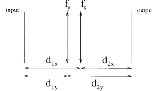
According to the above result, the x and y directions can be considered independently of each other, since the kernel given in Eqs.~29! is separable. Hence if two optical setups that achieve 1-D linear canonical transforms are put together, one can implement the desired 2-D fractional Fourier transform. The sug-gested optical system is shown in Fig. 3.

The parameters of the type 1 system are as follows:

d1x5 bx2 ax l~bx22 gxax! , d2x5 bx2 gx l~bx22 gxax! , fx5 bx l~bx22 gxax! , (54) d1y5 by2 ay l~by 2_{2 g} yay! , d2y5 by2 gy l~by 2_{2 g} yay! , fy5 by l~by22 gyay! . (55)

It was discussed in Subsection 2.B that a 2-D frac-tional Fourier transform is indeed a special linear canonical system with the parameters

ax5 cot fxys22, gx5 cot fxys12, bx5 csc fxys1s2, (56) ay5 cot fyys2 2 , gy5 cot fyys1 2 , by5 csc fyys1s2. (57) When Eqs.~56! and ~57! are substituted into Eqs. ~54! and ~55!, the parameters of the fractional Fourier transforming optical system can be found. Even though the analysis is carried out by use of the inde-pendence of the x and y directions, the total length of the optical system is fixed. Thus the condition d1x1 d_2x5 d_x5 d_1y1 d_2y5 d_yshould always be satisfied. The other constraint to be satisfied is the positivity of the lengths of the free-space sections: d_1x, d_1y, d_2x, and d2y should always be positive. These two

con-straints restrict the set of linear canonical transforms that can be implemented. The solution to this prob-lem is to simulate anamorphic sections of free space. Such simulation provides us with the propagation of

d_xin the x direction and of d_yin the y direction, where

dxand dycan take negative values. This problem is

solved in Subsection 3.B.

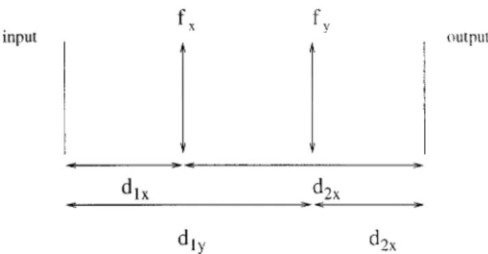
Two type 2 systems can also perform the desired 2-D linear canonical transforms. The parameters of the type 2 system are as follows:

dx5 1 lbx , f1x5 1 l~bx2 gx! , f2x5 1 l~bx2 ax! , (58) dy5 1 lby , f1y5 1 l~by2 gy! , f2y5 1 l~by2 ay! . (59) If Eqs.~56! and ~57! are substituted into Eqs. ~58! and ~59! we have the parameters for the fractional Fou-rier transform, which is indeed a linear canonical transform.

The optical setup shown in Fig. 4, with the

param-Fig. 3. Type 1 system that realizes 2-D linear canonical trans-forms.

(8)

eters given in Eqs.~58! and ~59!, implement the 2-D linear canonical transform. In this optical setup the constraint becomes dx5 dy5 d, which is even more

restrictive than that for type 1 systems. The terms

dxand dycan again be negative. To overcome these

difficulties, we try to design an optical setup that simulates anamorphic sections of free space.

C. Simulation of Anamorphic Sections of Free Space

While designing optical setups that implement 1-D linear canonical transforms we treat the lengths of the free-space sections as free parameters. But some linear canonical transforms specified by the pa-rametersa, g, and b might require the use of free-space sections with negative length. This problem is again encountered in the optical setups that achieve 2-D linear canonical transforms. Besides, the 2-D optical systems require different propagation dis-tances in the x and the y directions. To implement all possible 1-D and 2-D linear canonical transforms, we design an optical system that simulates the de-sired free space suitable for our purposes. The op-tical system shown in Fig. 5, which comprises a Fourier block, an anamorphic lens, and an inverse Fourier block, simulates 2-D free space with the prop-agation distance dxin the x direction and dyin the y

direction. We call the optical system shown in Fig. 5 an anamorphic free-space system. When the analy-sis of the system illustrated in Fig. 5 is carried out, the relation between the input light distribution f~x,

y! and the output light distribution g~x, y! is given as g~x, y! 5 C

*

2` `

*

2` `

exp@ip~x 2 x9!2_yld

x 1 ~y 2 y9!2_yld y#f~x9, y9!dx9dy9, (60) where dx5 s4 l2_f x , dy5 s4 l2_f y , (61)

and s is the scale of the Fourier and the inverse Fourier blocks. The terms fxand fycan take any real

value, including negative ones. Thus it is possible to obtain any combination of dx and dy by use of the

optical setup depicted in Fig. 5. The anamorphic lens, which is used to control dxand dy, can be

com-posed of two orthogonally situated cylindrical thin lenses with different focal lengths. The Fourier block and the inverse Fourier block are 2f systems with a spherical lens between two sections of free space. Thus a section of free space uses two cylin-drical and two spherical lenses.

The system represented in Fig. 5 simulates 2-D anamorphic free space. The same configuration is again valid for the 1-D case. When only one lens is used with the 1-D Fourier and inverse Fourier blocks it is possible to simulate propagation with negative distances. When the free-space sections in the type 1 and type 2 systems are replaced with the optical setup of Fig. 5, optical implementation of all separa-ble linear canonical transforms can be realized.

Both type 1 and type 2 systems can be used to implement all combinations of orders when the free-space sections are replaced with sections of anamor-phic free space. We have no residual phase factors at the output. Also, the scale parameters can be specified by the designer. Thus by use of type 1 and type 2 systems all combinations of the orders axand

aycan be implemented with full control of the scale

parameters s1, s2and the phase factors px, py.

4. Other Optical Implementations of Two-Dimensional Fractional Fourier Transforms

In Section 3 we presented a method for implementing the fractional Fourier transform optically. All com-binations of axand aycan be implemented with the

proposed setups; however, both systems use six cy-lindrical lenses. In this section we consider simpler optical systems having fewer lenses and try to see the limitations of these systems. We do not attempt to exhaust all possibilities but offer several systems that we believe may be useful. Since the problem is solved in the x and y directions independently, one lens is not adequate for controlling both directions. So the simplest setup that we consider has two cylin-drical lenses.

A. Two-Lens Systems

1. Setup with Six Design Parameters

This setup has the following parameters:

• Parameters specified by the designer: f_x, f_y,

s1, s2, px, py.

Fig. 5. Optical system that simulates anamorphic free-space propagation.

(9)

• Design parameters: f_x, f_y, d_1x, d_1y, d_2x, d_2y.

• Uncontrollable outcomes: None.

The optical setup shown in Fig. 5 has six design parameters, and we also want to specify six param-eters here. It is possible to solve the design param-eters in terms of the desired paramparam-eters determined by the designer. However, to produce a realizable setup, we should satisfy the following constraints:

• The total length of the system should be the same in both directions: d1x1 d2x5 d1y1 d2y.

• The lengths of all free-space sections should be positive: d1x$ 0, d1y$ 0, d2x$ 0, and d2y$ 0.

These constraints are too restrictive, and the range of orders a_xand a_ythat can be implemented is small. Thus we have to reduce the number of parameters that we want to control. This method is considered in Subsection 4.A.2.

2. Setup with Fewer Parameters

This system has the following parameters:

s1, s2.

• Design parameters: f_x, f_y, d_1x, d_1y, d_2x, d_2y.

• Uncontrollable outcomes: px, py.

In this design both the orders and the scale param-eters can be specified. For the given parametersf_x, fyand s1, s2, the design parameters are

d1x5 d1y5 d15 s12~sin fy2 sin fx! l~cos fy2 cos fx! , (62) d2x5 d2y5 d25 s1s2sin~fx2 fy! l~cos fy2 cos fx! , (63) fx5 s12s2sin~fx2 fy!

l~s12 s2cosfx!~cos fy2 cos fx!

, (64)

fy5

s12s2sin~fx2 fy!

l~s12 s2cosfy!~cos fy2 cos fx!

, (65)

and the phase factors at the output plane turn out to be

px5

$s2~cos fy2 cos fx! 1 s1@1 2 cos~fy2 fx!#%

s1s22sin~fx2 fy!

, (66)

py5

$s2~cos fy2 cos fx! 1 s1@cos~fy2 fx! 2 1#%

s1s22sin~fx2 fy!

. (67) In this optical setup d₁and d₂should always be pos-itive~see Fig. 6!. But for some values of fx,fy, s1,

and s₂, the values of d₁ and d₂ may turn out to be negative. In such cases we would have to deal with virtual objects, virtual images, or both. This would require the use of additional lenses. To avoid this we must require that d₁ and d₂ be positive. This condition will restrict the ranges of axand aythat can

be realized. These ranges can be maximized if the x or the y axis is flipped. For instance, if the given values of d1x, d2x, d1y, and d2ymake s1 negative for

fx5 60 and fy5 30, we flip one of the axes. This

transform is equivalent to the fractional Fourier transform, withfx5 60 and fy5 210, followed by a

flip of the y axis or to the fractional Fourier trans-form, withfx5 240 and fy5 30, followed by a flip of

the x axis. ~This is because a second-order trans-form corresponds to a flip of the coordinate axis.! To implement some orders we must flip both axes. Fig-ure 7 shows the necessary flip~s! required to realize different combinations of orders.

The above system allows us to specify the orders and the scale parameters. However, the phase fac-tors are arbitrary and out of our control. We should examine four-lens systems if we wish to control the orders, the scale parameters, and the phase factors at the same time.

B. Four-Lens Systems

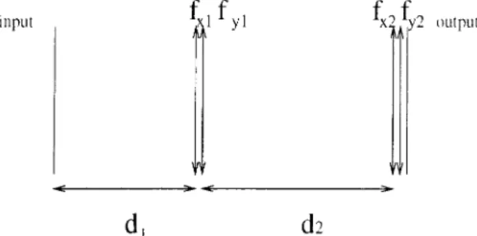
1. Setup with Adjustable Length

We continue our discussion with the setup shown in Fig. 8:

• Parameters specified by the designer: fx, fy,

s₁, s₂, p_x5 p_y5 0.

Fig. 6. Optical setup with two cylindrical lenses and three sec-tions of free space.

Fig. 7. Sections A: Neither axis flipped. Sections B: x axis

flipped. Sections C: y axis flipped. Section D: Both axes flipped.

(10)

• Design parameters: d₁, d₂, f_x1, f_y1, f_x2, f_y2.

In this configuration we use the optical setup de-picted in Fig. 8. In our design with two lenses ~Sub-section 4.A!, we managed to design an optical setup that implements the 2-D fractional Fourier transform with the orders and scale parameters we desired. However, additional phase factors at the output plane turned out to be arbitrary. If two cylindrical lenses are added to the output plane of the two-lens system, it is possible to remove the additional phase factor at the output. In the optical setup of Fig. 8,

d1, d2, fx1, and fx2have the same expressions as those

for the two-lens system. Thus Fig. 7 is again valid and shows the necessary flips:

d1x5 d1y5 d15 s1 2_{~sin f} y2 sin fx! l~cos fy2 cos fx! , (68) d2x5 d2y5 d25 s1s2sin~fx2 fy! l~cos fy2 cos fx! , (69) fx15 s1 2 s2sin~fx2 fy!

l~s12 s2cosfx!~cos fy2 cos fx!

, (70)

fy15

s12s2sin~fx2 fy!

l~s12 s2cosfy!~cos fy2 cos fx!

, (71)

fx25

s1s2 2

sin~fx2 fy!

l$s2~cos fy2 cos fx! 1 s1@1 2 cos~fy2 fx!#%

, (72)

fy25

s1s22sin~fx2 fy!

l$s2~cos fy2 cos fx! 1 s1@cos~fy2 fx! 2 1#%

. (73) This optical setup implements the 2-D fractional Fou-rier transform with the desired orders, scale param-eters, and phase factors.

2. Setup with Fixed Length

s1, s2, d1, d2, d3.

• Design parameters: f_x1, f_y1, f_x2, f_y2.

• Uncontrollable outcomes: px, py.

For practical purposes one may want to use a fixed system in which the lengths of all free-space sections are fixed. For example, Ref. 26 reports that the 2-D fractional Fourier transform is implemented by use of cylindrical lenses with dynamically adjustable focal lengths in a fixed system. Both the locations of the lenses and the total length of the system are fixed. The only design parameters are the focal lengths of the lenses, which can be changed dynamically.

Here we add one more section of free space to the system shown in Fig. 8 and obtain the setup shown in Fig. 9. This fixed system exerts no control over the phase factors, while the orders and the scale param-eters can be specified by the designer. The param-eters are fx15 s1s2d2sinfxyl 2 ~s2ys1!d1d2cosfx ~s2ys1!~d11 d2!cos fx2 s1s2sinfxyl 1 d3 , (74) fy15 s1s2d2sinfyyl 2 ~s2ys1!d1d2cosfy ~s2ys1!~d11 d2!cos fy2 s1s2sinfyyl 1 d3 , (75) fx25 d2d3 ~s2ys1!d1cosfx2 s1s2sinfxyl 1 d21 d3 , (76) fy25 d2d3 ~s2ys1!d1cosfy2 s1s2sinfyyl 1 d21 d3 , (77) and the additional phase factors turn out to be

px5 2cos fx1 s2 s1sinfx

S

12d1 fx1 2d1 fx2 2d2 fx2 1d1d2 fx1fx2

D

, (78) py5 2cos fy1 s2 s1sinfy

S

12d1 fy1 2d1 fy2 2d2 fy2 1d1d2 fy1fy2

D

. (79) This optical setup can be used to realize all combina-tions of a_xand a_y; however, there are additional un-controllable phase factors observed at the output plane.

C. Six-Lens System

Fig. 8. Optical setup with four cylindrical lenses and two sections of free space.

Fig. 9. Optical setup with four cylindrical lenses and three sec-tions of free space.

(11)

• Parameters specified by the designer: fx, fy,

s1, s2, d1, d2, d3, px5 py5 0.

• Design parameters: fx1, fy1, fx2, fy2.

The modified type 1 and type 2 systems use six cy-lindrical lenses. However, the lengths of the free-space sections are not fixed. For practical purposes, as we mentioned in Subsection 4.B.2, one may want to use a fixed system. To have control over all the parameters, we require a six-lens system. The de-sign that we made using the four-lens fixed system has two uncontrollable outcomes: pxand py. If two

cylindrical lenses are added to the output plane, full control over all parameters is achieved.

The system parameters fx1, fy1, f2x, and fy2are the

same as those for the four-lens fixed system. The focal lengths of the additional lenses are

fx35 1 lpx , (80) fy35 1 lpy . (81)

Thus the fixed optical system shown in Fig. 10 can be used to implement the desired fractional Fourier transform.

5. Conclusion

We have presented a systematic treatment of the 2-D fractional Fourier transform and its optical imple-mentation. We have provided design equations for a system composed of four cylindrical lenses, in which the user can specify the transform orders in two di-mensions, the input and output scale parameters, and the residual phase factors appearing at the out-put plane. Many other systems with fewer or more lenses and with less or more flexibility when specify-ing parameters have also been discussed.

The systems we discussed in Section 3 are good for realizing arbitrary linear canonical transforms. Such transforms are a more general class of trans-forms than the fractional Fourier transtrans-forms. References

1. H. M. Ozaktas and D. Mendlovic, “Fourier transforms of frac-tional order and their optical interpretation,” Opt. Commun.

101, 163–169_~1993!.

2. D. Mendlovic and H. M. Ozaktas, “Fractional Fourier

trans-forms and their optical implementation I,” J. Opt. Soc. Am. A

10, 1875–1881~1993!.

3. H. M. Ozaktas and D. Mendlovic, “Fractional Fourier trans-forms and their optical implementation II,” J. Opt. Soc. Am. A

10, 2522–2531~1993!.

4. A. W. Lohmann, “Image rotation, Wigner rotation, and the fractional order Fourier transform,” J. Opt. Soc. Am. A 10, 2181–2186~1993!.

5. D. Mendlovic, H. M. Ozaktas, and A. W. Lohmann, “Graded-index fibers, Wigner-distribution functions, and the fractional Fourier transform,” Appl. Opt. 33, 6188 – 6193~1994!. 6. H. M. Ozaktas and D. Mendlovic, “Fractional Fourier optics,”

J. Opt. Soc. Am. A 12, 743–751_~1995!.

7. P. Pellat-Finet, “Fresnel diffraction and the fractional-order Fourier transform,” Opt. Lett. 19, 1388 –1390~1994!. 8. P. Pellat-Finet and G. Bonnet, “Fractional order Fourier

trans-form and Fourier optics,” Opt. Commun. 111, 141–154~1994!. 9. D. Mendlovic, H. M. Ozaktas, and A. W. Lohmann, “Fractional

correlation,” Appl. Opt. 34, 303–309_~1995!.

10. L. M. Bernardo and O. D. D. Soares, “Fractional Fourier trans-forms and imaging,” J. Opt. Soc. Am. A 11, 2622–2626~1994!. 11. L. M. Bernardo and O. D. D. Soares, “Fractional Fourier trans-forms and optical systems,” Opt. Commun. 110, 517–522 ~1994!.

12. H. M. Ozaktas and D. Mendlovic, “Fractional Fourier trans-form as a tool for analyzing beam propagation and spherical mirror resonators,” Opt. Lett. 19, 1678 –1680~1994!. 13. T. Alieva, V. Lopez, F. Agullo-Lopez, and L. B. Almedia, “The

fractional Fourier transform in optical propagation problems,” J. Mod. Opt. 41, 1037–1044_~1994!.

14. M. A. Kutay, H. M. Ozaktas, L. Onural, and O. Arikan, “Op-timal filtering in fractional Fourier domains,” in Proceedings of

the 1995 IEEE International Conference on Acoustics, Speech, and Signal Processing~Institute of Electrical and Electronics

Engineers, New York, 1995!, Vol. 12, pp. 937–940.

15. M. A. Kutay, H. M. Ozaktas, O. Arikan, and L. Onural, “Op-timal filtering in fractional Fourier domains,” IEEE Trans. Signal Process. 45, 1129 –1143~1997!.

16. H. M. Ozaktas, O. Arikan, M. A. Kutay, and G. Bozdagi, “Dig-ital computation of the fractional Fourier transform,” IEEE Trans. Signal Process. 44, 2141–2150~1996!.

17. R. G. Dorsch, A. W. Lohmann, Y. Bitran, D. Mendlovic, and H. M. Ozaktas, “Chirp filtering in the fractional Fourier do-main,” Appl. Opt. 33, 7599 –7602_~1994!.

18. D. Mendlovic, Z. Zalevsky, A. W. Lohmann, and R. G. Dorsch, “Signal spatial-filtering using the localized fractional Fourier transform,” Opt. Commun. 126, 14 –18_~1996!.

19. A. W. Lohmann, Z. Zalevsky, and D. Mendlovic, “Synthesis of pattern recognition filters for fractional Fourier processing,” Opt. Commun. 128, 199 –204_~1996!.

20. Z. Zalevsky and D. Mendlovic, “Fractional Wiener filter,” Appl. Opt. 35, 3930 –3936~1996!.

21. D. F. McAlister, M. Beck, L. Clarke, A. Mayer, and M. G. Raymer, “Optical phase retrieval by phase-space tomography and fractional-order Fourier transforms,” Opt. Lett. 20, 1181– 1183~1995!.

22. J. Garcia, D. Mendlovic, Z. Zalevsky, and A. Lohmann, “Space-variant simultaneous detection of several objects by the use of multiple anamorphic fractional-Fourier-transform filters,” Appl. Opt. 35, 3945–3952_~1996!.

23. B. Barshan, M. A. Kutay, and H. M. Ozaktas, “Optimal filter-ing with linear canonical transformations,” Opt. Commun.

135, 32–36~1997!.

24. H. M. Ozaktas, “Repeated fractional Fourier domain filtering is equivalent to repeated time and frequency domain filtering,” Signal Process. 54, 81– 84~1996!.

25. H. M. Ozaktas and D. Mendlovic, “Every Fourier optical

sys-Fig. 10. Optical system with six lenses and three sections of free space.

(12)

tem is equivalent to consecutive fractional Fourier domain filtering,” Signal Process. 54, 81– 84~1996!.

26. M. F. Erden, H. M. Ozaktas, A. Sahin, and D. Mendlovic, “Design of dynamically adjustable fractional Fourier trans-former,” Opt. Commun. 136, 52– 60~1997!.

27. D. Mendlovic, Y. Bitran, C. Ferreira, J. Garcia, and H. M. Ozaktas, “Anamorphic fractional Fourier transforming— optical implementation and applications,” Appl. Opt. 34, 7451– 7456~1995!.

28. A. Sahin, H. M. Ozaktas, and D. Mendlovic, “Optical imple-mentation of the two-dimensional fractional Fourier transform with different orders in the two dimensions,” Opt. Commun.

120, 134 –138,~1995!.

29. A. Sahin, “Two-dimensional fractional Fourier transform and its optical implementation,” M.S. thesis~Bilkent University, Ankara, Turkey, 1996!.

30. Y. B. Karasik, “Expression of the kernel of a fractional Fourier transform in elementary functions,” Opt. Lett. 19, 769 –770 ~1994!.

31. L. B. Almeida, “The fractional Fourier transform and time– frequency representations,” IEEE Trans. Signal Process. 42, 3084 –3091~1994!.

32. V. Namias, “The fractional order Fourier transform and its application to quantum mechanics,” J. Inst. Math. Its Appl. 25, 241–265~1987!.

33. A. C. McBride and F. H. Kerr, “On Namias’s fractional Fourier transform,” IMA J. Appl. Math. 39, 159 –175.

34. H. M. Ozaktas, B. Barshan, D. Mendlovic, and L. Onural, “Convolution, filtering, and multiplexing in fractional Fourier domains and their relation to chirp and wavelet transforms,” J. Opt. Soc. Am. A 11, 547–559~1994!.

35. M. J. Bastiaans, “Wigner distribution function and its appli-cation to first-order optics,” J. Opt. Soc. Am. A 69, 1710 –1716 ~1979!.

36. K. B. Wolf, “Construction and properties of canonical trans-forms,” in Integral Transforms in Science and Engineering ~Plenum, New York, 1979!, Chap. 9.

37. B. E. A. Saleh and M. C. Teich, Fundamentals of Photonics ~Wiley, New York, 1991!.

38. M. J. Bastiaans, “The Wigner distribution applied to optical signals and systems,” Opt. Commun. 25, 26 –30~1978!. 39. M. J. Bastiaans, “The Wigner distribution function and

Ham-ilton’s characteristics of a geometric-optical system,” Opt. Commun. 30, 321–326~1979!.

40. M. J. Bastiaans, “Propagation laws for the second-order mo-ments of the Wigner distribution in first-order optical sys-tems,” Optik~Stuttgart! 82, 173–181 ~1989!.

41. M. J. Bastiaans, “Second-order moments of the Wigner distri-bution function in first-order optical systems,” Optik ~Stutt-gart! 88, 163–168 ~1991!.