The interface of buffer design and cyclic scheduling decisions in deterministic flow lines

(1)

Annals of Operations Research 50(1994)295-317 295

The interface of buffer design and cyclic scheduling

decisions in deterministic flow lines

Selcuk Karabati

Faculty of Business Administration, Management Department, Bilkent University, 06533 Bilkent, Ankara, Turkey

and

Panagiotis Kouvelis

The Fuqua School of Business, Duke University, Durham, NC 27706, USA

In this paper, we address some issues on the interface of buffer design and cyclic scheduling decisions in a multi-product deterministic flow line. We demonstrate the importance of the above interface for the throughput performance of the flow line. In particular, we point out that the use of sequence-independent information, such as workload distribution and variability in processing times among stations, is not adequate to decide the optimal buffer configuration of the flow line. We formulate the buffer design problem for a fixed sequence of jobs as a general resource allocation problem, and suggest two effective heuristics for its solution. For the simultaneous buffer design and cyclic scheduling problem, we suggest an iterative scheme that builds on the effectiveness of the above heuristics. One of the side results of our extensive computational studies on this problem is that the general guidelines of buffer design in single-product flow lines with stochastic processing times are not directly transferable to the multi- product deterministic flow line environment.

1. Introduction

F l o w lines are the basic manufacturing processes for companies competing on a high volume, low cost manufacturing task. The inherent efficiencies o f f l o w lines can only be achieved by thorough analyses o f design problems, e.g. allocation o f buffers between stations, and operational decisions, e.g. scheduling o f parts. In this paper, we address some issues on the interface o f buffer design and scheduling decisions in a deterministic flow line. We consider a flow line with finite/infinite capacity buffers between the stations which produces a set o f products under a cyclic scheduling policy.

The cyclic scheduling approach for flow lines is based on the idea of repetitively producing a small set o f items. Each set has the items to be produced in the same proportions as the production requirements of the system over a planning horizon © J.C. Baltzer AG, Science Publishers

(2)

296 S. Karabati, P. Kouvelis, Buffer design and cyclic scheduling decisions

or as the assembly requirements of an end product. We now sequence parts in a rather small production set and then simply repeat the same part sequence (for a detailed discussion of the cyclic scheduling problem, we refer the reader to McCormick et al. [13], and Karabati and Kouvelis [10]). Some of the advantages of cyclic scheduling policies over conventional scheduling techniques for such environments are mentioned in the research literature (Matsuo [12], Lee and Posner [11]) and include benefits such as better machine utilization, smoother finished goods inventory levels, and implementation convenience due to the simplicity of cyclic schedules. The problem of buffer design in flow lines has been extensively studied in the literature. As surveyed by Sarker [ 17] and by Smunt and Perkins [18], researchers have considered the buffer design problem in a variety of contexts. A major part of the research has concentrated on lines with a single product and stochastic processing times. Researchers normally have dealt with flow line systems where station service time variability is described by normal or exponential distributions. Although the exponential distribution is not a particularly good representative of actual service time variability, it allows mathematical manipulation. Models using exponential distribution and relying on a queueing theoretic approach have been reported by, among others, Hunt [8], Hillier and Boling [3,4], Rao [16]. Recently, Hillier et al. [5], and Hillier and So [6] have addressed the buffer allocation problem in a single-product flow line with stochastically identical and independent stations. Their results show that the "bowl-effect", whereby the center stations are given preferential treatment through more storage spaces, is more pronounced with higher variability in the processing times. This conclusion is in parallel with the simulation results of Conway et al. [2] and Yamashina and Okamura [20].

The above literature (both analytical and simulation studies) has mostly concentrated on single-product environments. For such environments, the source of variability in processing times is the stochastic nature of the operations undertaken at the various stations, and the presence of buffers helps to reduce the adverse effects of stochastic variability of processing times on the throughput rate of the line. In multi-product stochastic flow lines, the source of variability is not only the stochastic variability of each job but also the variability in processing times across the jobs. In other words, even in the absence of stochastic variability in processing times, in a multi-product environment there exists variability of processing times at each station due to the wide mix of jobs processed there. Therefore, the presence of buffers can help in alleviating station starvation or blocking instances.

The difficulty in analyzing multi-product stochastic flow lines has led to the development of models that assume, for the convenience of analytical tractability, single-product environments, exponential distribution of processing times, and often ignore the interface of buffer design/scheduling decisions on the throughput performance of the flow line. However, the current flow line environments are multi-product, and most of the operations are performed by numerically controlled machining centers that exhibit almost deterministic processing time behavior. Even more, current simulation studies of automatic flow line environments point out the significant

(3)

S. Karabati, P. Kouvelis, Buffer design and cyclic scheduling decisions 297

benefits in throughput performance from the simultaneous consideration of buffer design and sequencing issues (see Park and Steudel [15]). As the cycling scheduling approach allows the manager to extend the planning horizon of the sequencing problem (a cyclic scheduling policy can be used to meet monthly or quarterly demand requirements), and since the alteration of the buffer configuration for many flow line environments involves only the use of additional space and storage bins between stations, the use of buffer configurations that account for the decided cyclic scheduling policy is within the implementation capabilities of the manager. The usual hierarchical approach for solving the above problems, with buffer capacity being determined without consideration to job sequencing and then an algorithm for job sequencing being developed, leads to excessive capacity for a desired system throughput rate (see Park and Steudel [15]). Motivated by the above described trends in the operations of flow lines, and the suboptimality of the hierarchical decision-making framework used for these environments, we proceeded to develop a modeling framework that adequately captures the buffer design/cyclic sequencing interface issue.

In this paper, we approach the buffer design problem using the modeling framework of a multi-product flow line with deterministic processing times. The exclusion of stochastic processing times reduces the complexity of the problem to some extent; however, as we will discuss in the following sections of the paper, the problem is still a very difficult one. We discuss the extent to which the results of the previous research on single-product flow lines with stochastic processing times apply to the multi-product flow line with deterministic processing times. We note that in both modeling frameworks there exists a variability component in the processing times; however, in the multi-product deterministic flow line problem, the variability arises from the differences between the processing requirements of different products. Within our framework, we suggest an effective iterative approach for simultaneous determination of buffer design and cyclic sequencing of jobs over a planning horizon.

This paper is organized as follows. In section 2, we present a brief overview of the cyclic scheduling problem, which serves as a necessary background for our further discussion. A formulation of the buffer design problem in a deterministic flow line and for a fixed sequence of jobs is presented in section 3. In section 4, through extensive numerical experimentation, we demonstrate the importance of the buffer design/cyclic sequencing interface for the throughput performance of the flow line. In section 5, we propose two effective approximate procedures for the buffer design under a fixed cyclic sequence of jobs. These procedures serve as the main building block for the development of an iterative solution procedure for the simultaneous buffer design and scheduling problem. This iterative procedure is discussed in section 6. The effectiveness of the procedure is demonstrated through extensive numerical experiments. Finally, in section 7, we present our concluding remarks.

(4)

2. Cyclic scheduling in flow lines

In this section, we present a brief overview of the cyclic scheduling problem in a deterministic flow line. The flow line consists of m stations in series, Ml, • • •, Mm, with finite or infinite capacity buffers between the stations. Let ri be the n u m b e r of units o f item Ii, i = 1 , . . . , l, required to meet a production target o f the line over a planning horizon, and r = (r t . . . rt) be the production requirement vector for all l different items produced in the line over the same horizon. If q is the greatest c o m m o n divisor of the integers r 1 .. . . . rt, then the vector

is referred to as the Minimal Part Set (MPS) (term introduced by Hitz [7]). MPS represents the smallest part set having the same properties as the production requirement vector. Under a cyclic scheduling policy, the flow line will repetitively produce MPSs, using the same sequence of jobs, i.e. items that form the MPS, for all part sets. We may also produce an integral multiple of MPS in a repetitive manner; however, without any loss of generality, we are going to confine our discussion to the production of MPSs.

Let n be the number of jobs in an MPS. We denote by Piy, i = 1 . . . n,

j = 1 . . . m, the processing time of job Ji on station My. T h e cyclic scheduling problem is to find the optimal sequence of jobs in a prespecified part set in order to optimize the throughput rate of the line, or equivalently its cycle time (i.e. the reciprocal of the throughput rate of the line). We are restricting our analysis to the operation of conventional flow lines (i.e. by-passing of stations by some jobs is not allowed). For references on flexible flow lines, which allow station by-passing by some jobs, see Hitz [7] and Wittrock [19].

Let us now consider the operation of the line under the cyclic scheduling approach. The units o f an MPS go through the system in a given order, followed by a second MPS in the same order and so on. An MPS schedule will be represented by permutation cr= (~r(1), or(2) . . . or(n)), where n is the number of jobs in the MPS and or(i) is the ith job in the processing order. Note that we restrict our analysis to permutation schedules only, i.e. no job passing is allowed once the MPS is released to the system. The ith job in the rth MPS is the rth repetition of job ~r(i) and is denoted by

CTr(i ).

Let us first consider a flow line with infinite capacity buffers. In this environment, the completion time C(crr(i),j) of job Crr(i) on station Mj can be found using the following recursive relationship (for similar representations of permutation schedules in flow shops, see Baker [1], and M o n m a and Rinnooy Kan [14]):

(5)

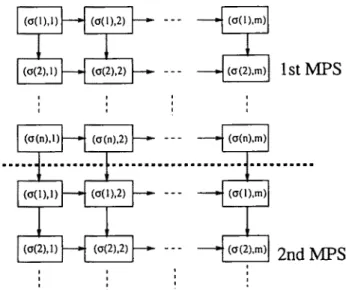
where C(ar(O),j) = C(Crr_1(n),j), r = 2, 3 . . . j = 1 . . . m and C ( c q ( 0 ) , j ) = 0, j = 1 . . . m, C(cyr(i), 0) = 0, i = 1 . . . n, r = 1, 2 . . . The recursive structure ( I ) can be equivalently represented, as pointed out by M o n m a and R i n n o o y Kan [14], by the directed graph depicted in fig. 1. Vertices (cry(i), j ) are defined for each element a ( i ) of the permutation, for r = 1, 2 . . . and each station Mj. Directed

a ) a i ) ! 1 ( I 1 I i 1 st M P S . . . . ... ... . . . ~ ~.m-~ 2 n d M P S u ) ) a I i ) a o i

Fig. 1. Directed graph representation of completion times: infinite capacity buffers case.

arcs are defined f r o m each vertex (Crr(i),j) towards (CYr(i + 1 ) , j ) and (ar(i),j + 1). For i = n, we use the convention (o'r(n + 1 ) , j ) = (err+l(1), j) to depict the cyclic nature of the schedule. A weight Pa(o,j is associated with each vertex. Given the above defined graph, the c o m p l e t i o n time C(c~r(i), j ) of j o b err(i) on station Mj is equal to the weight of the m a x i m u m - w e i g h t e d directed path f r o m (an(l), 1) to (err(i), j) in the graph, as follows immediately f r o m the recursive relationship (1). Next we would like to discuss how this framework can be extended to problems with finite capacity buffers. First, without any loss of generality, we m a y assume that all buffers have either zero capacity or infinite capacity, because we can represent each unit buffer location by a station at which all processing times are equal to zero. Thus, in order to extend the framework, we only need to find a way to handle the case where the buffer capacity between station Mj and Mj+I is equal to zero. T h e c o m p l e t i o n time of C(cy~(i),j) of the rth repetition of j o b or(i) on station Mj is n o w given by

C(Crr(i), j)

(6)

where C ( o ' r ( O ) , j ) = C ( o ' r - l ( n ) , j ) , r = 2, 3 . . . j = 1 . . . m and C(O-I(0),j) = 0, j = 1 . . . m, C(o-r(i), 0) = 0, i = 1 . . . n, r = 1, 2 . . . The difference between relationships (1) and (2) is due to the blocking of jobs in the presence of zero capacity buffers. In order to account for this in our graph-theoretic model, we define diagonal arcs from vertices ( o - r ( i ) , j + 1), i = 1 . . . n, to vertices (o-r(i + 1),j), as illustrated in fig. 2. This modeling approach allows C ( o ' r ( i ) , j ) to be f o u n d by

i i i i I t i I i i i I 1 st M P S i t t i i J t i J t i t

Fig. 2. Directed graph representation of completion times: zero capacity buffers case.

determining the weight of the m a x i m u m - w e i g h t e d path from vertex (o'1(1), 1) to (Or(i), j ) . However, in c o m p u t i n g the weight of a path between these two nodes, the weight of a vertex which is entered via one of the diagonal arcs is taken to be zero, as is required by relationship (2).

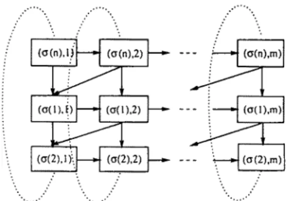
The performance criterion we want to optimize is the throughput rate of the flow line, or equivalently its cycle time. To define the cycle time of a flow line in our m o d e l i n g framework, we need to introduce the notion of a cylinder f o r m e d by the directed graph of a single MPS. The easiest way to introduce this notion is to present a graphical equivalent of the cylinder. Figure 3 depicts the cylinder f o r m e d by the directed graph of a single MPS. Then, the total weight of the m a x i m u m - w e i g h t e d path around a cylinder formed by the directed graph of a single MPS equals the cycle time (see M c C o r m i c k et al. [13]). The weight F(o', ~') of a path "t" around the cylinder (i.e. a chain of vertices that starts at a particular vertex and ends at the same vertex after completing one tour around the cylinder), with the cylinder being f o r m e d using the permutation schedule o" (as in fig. 3), can be expressed in the following way:

(7)

° • . . • . ••.... ." ; .."

\ .: • .r

Fig. 3. Directed graph representation of the MPS cylinder.

w[ H w~

F(cr, I:)= ,~ Ptr(l),k + ~ Pcr(2),k + " " + ~ Pa(n)Jc, (3)

k=w~n k=w[ k=wfn_l

where w = (w~ r . . . w~) is a unique set of integers. For any given path t, we can determine the unique set of integers w r = (w[ . . . w~) to represent the weight of the path using the above functional form. We will illustrate this point using the following example.

EXAMPLE

Consider a 3-jobs per MPS, 3-station problem, where the buffer capacity between stations 1 and 2 is infinitely large and the buffer capacity between stations 2 and 3 is zero. The cylinder of this problem is presented in fig. 4. We now consider

~ (c(1),3) [

llll ...

1

Fig. 4. Directed graph of the example problem.

the path 7, which is given by the dark lines in fig. 4. The weight of path 1: is equal to

(8)

302 S. Karabati, P. Kouvelis, Buffer design ~ d cyclic scheduling decisions

F(cr,

z) = po~(l),2 + Pa(1),3 + Pa(3),2.

Now, let w~= (3, 2, 2); then

3 2 2

F(tr, Z) = ~ Pa(1),k

+ ~ Pa(2),k

+ ~ Pa(3),k"

k=2 k=3 k=2

3. Formulation of the buffer design problem for a fixed sequence of jobs

We now present a formulation of the buffer design problem for a fixed sequence of jobs. Consider a flow line with m stations. Let N be the total number of buffers to be allocated, and

xi

be the number of buffers allocated between stations

Mi

and

Mi+l,

i = 1 . . . m - 1. Also, let T be the set of paths around the cylinder

formed in the resulting (m + N) station problem, where we treat each unit buffer location as a station on which all processing times are equal to zero. For a given buffer allocation X, X = (xl, x2 . . . x,,,_l), the length of path z, z E T, is denoted

by

f(z, X)

and is given by the following relationship:

w mfkI

}

f ( z , X ) = ~ k~__lPl,kl i = ~ ( x t + l ) + l i=wfn 1=1 wn ~ m f k-I }

+ ' " +

X

X P n , k l | i :

X ( X l + 1 ) + 1 ' i=w~n_lk=l [ /=1 (4)

where

Pi,j

is the processing time of job Ji on station

My,

and 1{i =

Y.~Z~(x t +

1) + 1} is an indicator function. This function is equal to I, if (Y~t~-~

xi)

m ~ y buffers have been allocated into locations before station

Mk,

and 0 otherwise. This representation o f f ( z , X), which is a direct extension of the framework presented in section 2, is illustrated by the following example.

EXAMPLE

We consider a 3-station problem with a unit capacity buffer location. Let z r = 1. If the buffer location is placed after the first be a path with w~ = 2 and

w n

station, i.e. xl = I and x2 = 0, the contribution of the first job to the weight of path z is equal to Pl. 1. On the other hand, if the buffer location is placed between stations 2 and 3, the contribution of the first job is equal to PI,I

+Pl,2.

In eq. (4), the contribution of the first job is given by

k~=lPl,kl i

=

(X l +

1) + 1 .

(9)

When xl = 1 and x2 = 0, the above quantity is equal to P1,1; similarly, when x 1 = 0 and x2 = 1, the above quantity is equal to Pl,l +Pl,2.

Since the throughput rate of the line is equal to the reverse of the cycle time, and the cycle time is equal to the length of the longest path in T, the problem of buffer allocation can be formulated as follows:

(BAL)

f = min F ( X )

m - I

subject to ~_~ x i = N,

i=1

x i > 0 and integer, i = 1 .. . . . m - 1,

where F(X) = maxrerf('r, X). (BAL) is a resource allocation problem with integer variables. The general resource allocation problem with integer variables in NP- hard (Ibaraki and Katoh [9]). The objective function F(X) is not separable in xi's, and it is neither convex nor concave in X. Thus, (BAL) can be safely characterized as a general resource allocation problem with the implied consequence of being NP- hard. The following simple examples demonstrate the lack of any nice convexity (or concavity) properties of F(X).

EXAMPLES

Consider the 3-job 2-station problems with processing times given in tables 1

Table 1 Table 2

Example problem. Example problem.

and 2. Stations Stations 1 2 1 2 1 100 100 1 90 1 Jobs 2 1 3 Jobs 2 10 100 3 2 1 3 2 3

Let cr= (1, 2, 3) be the fixed schedule. The cycle time of the problem given in table 1 is equal to 203 when we have a zero capacity buffer between the stations. When the buffer capacity is equal to 1, the cycle time is 200. However, when we have 2 buffers between the stations, the cycle time becomes 104. Therefore, F(X) is not convex in X. Similarly, consider the problem given in table 2. The cycle time with no buffers between the stations is 200. When we have a single buffer between the stations, the cycle time is 110. With the allocation of another buffer, the cycle time becomes 104; therefore, F(X) is not concave in X.

(10)

To further illustrate the ill-structured nature of this problem, we demonstrate below through a simple example the lack of any reversibility property for our problem. The reversibility property is an important, and handy, concept for single- product flow lines with stochastic processing times, and it states that the production capacities (i.e. throughput rates) of a line and its dual line (formed by using the reverse sequence of stations) are identical (see Yamazaki and Sakasegawa [21]). Unfortunately, for our multi-product deterministic flow line operated under a cyclic scheduling policy, the dual (mirror image) line does not necessarily have the same throughput rate as the original line. The following example demonstrates this point.

EXAMPLE

Consider the 2-job 3-station problem with zero capacity buffers given in table 3 and its mirror image in table 4. The original problem has a cycle time of 14, whereas the cycle time of the mirror image problem is 12. Note that increasing the mirror image problem, we reversed the sequence of jobs; however, since the 2- job cyclic scheduling problem has the same cycle time for both possible sequences

of jobs, the result is sequence independent.

Table 3

Example problem.

Table 4

Mirror image of the example problem.

Stations Stations

I 2 3 1 2 3

Jobs 1 2 6 6 Jobs 1 1 2 6

2 6 2 1 2 6 6 2

. The importance of the interface of buffer design and scheduling decisions in deterministic flow lines

The (BAL) formulation of the previous section clearly indicates that the sequencing decisions affect the selection of the throughput maximizing buffer configuration of the flow line. The importance, however, of the interface of buffer design and cyclic scheduling decisions is not immediately apparent from the above formulation. Does this interface constitute a second-order effect for the throughput performance of the line, and as such it can be ignored, with the immediate implication that the two decisions can be treated independently? Or, is the impact of this interface on the flow line's throughput significant enough to justify an attempt of handling the two decisions simultaneously? To answer the above questions, we pursued the following three avenues:

(11)

(a) We examined whether sequence-independent information, such as workload distribution and processing time variability at each station, would be adequate to identify the optimal buffer configuration.

(b) We examined the average throughput performance of specific buffer configurations for a variety of schedules.

(c) We examined the degree of transferability of the results found in the stochastic buffer design literature to the deterministic flow line environment. Our performance measure for evaluating the buffer allocation rules is the throughput rate of the flow line.

We discuss the results of our investigation in the next three subsections.

4.1. USE OF SEQUENCE-INDEPENDENT INFORMATION TO SELECT THE OPTIMAL BUFFER

CONFIGURATION FOR DETERMINISTIC FLOW LINES

In single-product flow lines with stochastic processing times, the characteristics of the flow line under consideration (i.e. information on workload distribution and variability in processing times) play an important role in developing guidelines for optimal buffer design. For example, in flow lines with identical stations, i.e. stations with similar workloads and variability in processing times, the inverted "bowl- shaped" buffer allocation has been shown to be very effective (Hillier et al. [5]). Similarly, in flow lines with balanced stations, i.e. stations with equal workloads and unequal variability in processing time, the stations with large variability in processing times should have large buffers for both input and output (Conway et al. [2]).

In this section, we will attempt to answer the questions whether similar guidelines can be developed for multi-product deterministic flow lines using the information on workload distribution among stations and processing time variabilities. The workload of a station is equal to the sum of the processing times of the operations that are going to be performed on this station. The processing time variability in our case is the variability due to the mix of jobs processed at a station. The processing time variability parameter used is the squared coefficient of variation. The squared coefficient of variation (scv) of a station is equal to the unbiased estimate of the variance of processing times divided by the square of the mean processing time on this station. These above two parameters are schedule independent, and therefore, if we can develop optimal buffer design rules based on these parameters, we do not have to consider the interface between the buffer design problems and scheduling decisions. In order to shed some light on this particular issue, we created 8- and 12-job, 6-station problems with a total of 4, 5 and 6 buffers to be allocated. In table 5, we report our results. We looked at 6 different problem classes, with each class being characterized by the workload distribution pattern and the squared coefficient of variation of the stations. Within each problem class, we looked at three different problem sets, with each set being characterized by the total number

(12)

Table 5

Number of instances that a buffer design was optimal over 50 different problems.

Problem Class No. of Optimal designs

class description buffers 8-job problems 12-job problems

llll0(10) 01120 (7) 4 02101 (7) 02020 (7) Balanced 02110 (6) 02110 (6) workloads 11111 (14) 11111 (12) scv= l.OO 5 11120 (6) 02111 (7) forall 01121 (5) 02120 (4) staUons 21111 (6) 12111 (9) 6 11121 (6) 11211 (8) 11211 (5) 11121 (7) IIII0(II) 01111 (14) 4 II011 (11) III01 (7) Balanced III01 (8) llll0 (6) workloads 11111 (21) 11111 (29) scv=0.50 5 11120 (5) 02111 (5) for all 21020 (4) 11120 (4) 11121 (13) 11211 (16) 6 11211 ( I ! ) 11121 (12) 12111(11) 12111 (9) C 11110(15) 01111 (12) 4 01II1 (10) 111t0(12) Balanced 10111 (10) 11011 (11) workloads I l I l l (40) 11111 (42) scv=0.25 5 10121 (2) 11120 (2) for all 21101 (2) 11201 (1), stations 11211 (12) 11121 (15) 6 11211 (12) 11211 (13) 21111 (10) 12111 (8) IIII0 (13) 02110 (13) 4 11200 (6) IIII0 (9) Inverted bowl- 01201 (5) 01210 (6) shaped workloads 12110(10) 11210 (8) scv=O.50 5 I1210 (4) 11111 (7) fo~all IIIII (4) 02120 (6) stations 21111 (6) 21210 (5) 6 12210 (6) 12120 (5) 12111 (5) 11220 (5) 01012 (15) I0111 (12) 4 10012 (9) 11011 (9) Bowl-shaped 10111 (7) 01012 (7) workloads 11012 (11) 10112 (8) scv=0.50 5 10112 (7) 21011 (6) for all 01013 (6) 11012 (6) smfions 11112 (17) 21012 (11) 6 20112 (16) 11112 (11) 10122(14) 20112 (10) Balanced workloads increasing scv's 0.25, 0.40 ... 0.85, 1.00 O l l l l (21) 01111 (23) 4 10111 (8) 01021 (6) 01021 (7) 01120,(4) ... I I I I I (16) 01121 (17) 5 01112(12) 01112(11) 01121 (8) 02111 (9) 11121 (16) 11121 (9) 6 11211 (9) 11112 (8) 11112 (6) 02031 (7)

(13)

of buffers to be allocated. For each problem set, we generated 50 problems using the parameters of the problem class and for each problem, we first randomly chose a schedule of jobs and then determined the optimal buffer allocation for this schedule by complete enumeration. For each problem set, we report the three most common optimal buffer designs and the number of problems for which each particular design has been the optimal buffer allocation. For example, in problem class A with balanced workloads and unit squared coefficients of variation, and for a total of 4 buffers to be allocated, buffer allocation X = (1, 1, 1, 1, 0) has been the optimal allocation in 10 problems out of 50 8-job problems. Similarly, buffer allocation X = (1, 2, 1, 0, 1) has been the optimal allocation in 7 problems out of 50 problems in the same problem set. The results of table 5 clearly indicate that, for most of the problem classes, no particular buffer design dominates other designs. This observation strongly suggests that the solution of the buffer design problem in multi-product flow lines depends also on information other than the schedule-independent information we have used in identifying the problem classes, and it constitutes a first indication that the buffer design and cyclic scheduling interface is important.

4.2. THROUGHPUT PERFORMANCE OF BUFFER CONFIGURATIONS FOR A VARIETY OF

JOB SEQUENCES

In this subsection, we explicitly consider the effects of scheduling decisions on optimal buffer design and attempt to quantify the relative importance of the scheduling decisions in terms of the throughput rate of the flow line. In table 6, we report our computational results. We looked at 6 different problem classes, with each class being characterized by the workload distribution pattern and the squared coefficient of variation of the stations (see table 5 for descriptions of problem classes). We concentrated on 8-job problems with a total of 6 buffers to be allocated. Our aim was to observe the throughput performance of the flow line for buffer configurations when 50 randomly generated sequences of 8 jobs are performed on it. For a specific job sequence and buffer configuration, we calculated a normalized throughput rate. In order to normalize the throughput rate of a problem, we divided it by the maximum throughput rate of the flow line with infinite capacity buffers between the stations. Note that in a flow line with infinite capacity buffers, all schedules have the same throughput rate (see Karabati and Kouvelis [10]). The information reported in the segment of the table that corresponds to a specific problem class is the following. The first row documents the throughput performance (normalized throughput rate) of the flow line when the optimal buffer configuration is implemented for each job sequence. The values in columns 1 to 3 are the maximum, minimum, and average normalized throughput rate of the optimal buffer configurations over the 50 random schedules. The observed standard deviation of the throughput rates over the 50 schedules is reported in column 4. In balanced workloads, unit squared coefficients of variation problem (problem class A in table 6), the maximum and minimum throughput rates achieved by 50 different schedules are 0.778 and

(14)

Table 6

Throughput performance of buffer configurations for a variety of job sequences (50 sequences).

Problem Throughput Deviation

class Design Max Min Mean S.D. Mean S.D. Optimal 0.778 0 . 6 5 1 0.714 0.029 - - 21111 0.765 0.577 0.663 0.041 7.07 5.97 A 11121 0.773 0.577 0.667 0.041 6.58 5.30 I 1211 0.756 0.577 0.672 0.039 5.94 4.74 Optimal 0.899 0.756 0.825 0.039 - - 11121 0.877 0.694 0.787 0.044 4.16 3.24 B 11211 0.864 0.694 0.790 0.043 4.24 3.49 12111 0.864 0.694 0.789 0.042 4.33 3.29 Optimal 1.000 0.835 0.923 0.043 - 21111 1.000 0.744 0.864 0.053 6.35 3.63 D 12210 0.956 0.772 0.852 0.048 7.63 4.89 21210 1.000 0.744 0.873 0.056 5.39 3.98 Optimal 1.000 0.864 0.935 0.034 - - 11112 1.000 0.804 0.904 0.051 3.36 4.11 E 20112 1.000 0.809 0.900 0.047 3.76 4.03 10122 0.981 0.787 0.876 0.048 6.32 4.26 Optimal 0.895 0.702 0.784 0.046 - - l 1121 0.822 0.629 0.732 0.054 6.51 5.31 F 11211 0.876 0.609 0.738 0.061 5.84 5.36 11112 0.881 0.609 0.742 0.060 5.34 4.51 Optimal 0.869 0.720 0.793 0.040 - - Mirror 21111 0.843 0.654 0.747 0.039 5.74 4.36 image of F a~ 12111 0.867 0.622 0.755 0.056 4.87 4.62 11211 0.850 0.618 0.737 0.057 7.06 5.03 a~ Mirror image of a problem class is obtained by reversing the order of stations.

0.651, r e s p e c t i v e l y , w h e n the o p t i m a l b u f f e r d e s i g n s f o r e a c h s c h e d u l e a r e u s e d . A c o m p a r i s o n o f m a x i m u m a n d m i n i m u m t h r o u g h p u t rates u n d e r o p t i m a l b u f f e r d e s i g n s in t a b l e 6 c l e a r l y d e m o n s t r a t e s the s i g n i f i c a n t e f f e c t o f s c h e d u l i n g on the t h r o u g h p u t rates.

F o r e a c h p r o b l e m c l a s s s e g m e n t in t a b l e 6, w e also p r e s e n t the p e r f o r m a n c e o f the m o s t c o m m o n b u f f e r d e s i g n s o f a p r o b l e m class, w h i c h are o b t a i n e d u s i n g e x p e r i m e n t s s i m i l a r to the o n e s p r e s e n t e d in s e c t i o n 4.1. F o r e x a m p l e , in 8 - j o b , 6- b u f f e r , b a l a n c e d w o r k l o a d s a n d unit s q u a r e d c o e f f i c i e n t s o f v a r i a t i o n p r o b l e m s , b u f f e r d e s i g n s X = (2, 1, 1, 1, 1), X = (1, 1, 1, 2, 1), a n d X = (1, 1, 2, 1, 1) ( p r o b l e m c l a s s A o f t a b l e 6) h a v e b e e n the m o s t c o m m o n , a n d t h e i r p e r f o r m a n c e o v e r 50 s c h e d u l e s a r e t a b u l a t e d in r o w s 2, 3, a n d 4, r e s p e c t i v e l y . In c o l u m n 5 o f t a b l e 6,

(15)

S. Karabati, P. Kouvelis, Buffer design and cyclic scheduling decisions 309

we present the percentage deviations of the throughput performances of these designs from the flow line performance when optimal buffer designs are used for the corresponding schedules. These results show that we may end up with considerably inferior throughput rate performances (more than 5% in most cases) if we do not take the scheduling decisions into account in allocating the buffers.

4.3. BUFFER DESIGN GUIDELINES FOR SINGLE-PRODUCT STOCHASTIC FLOW LINES

AND THEIR APPLICABILITY TO MULTI-PRODUCT DETERMINISTIC FLOW LINES As a last test on the importance of the interface of buffer design and scheduling decisions, we looked at the extent to which simple buffer design rules developed in the single-product stochastic flow line literature are valid (i.e. near optimal in terms of throughput performance) in our multi-product deterministic flow line environment. One of the most recent and comprehensive studies on buffer design rules for stochastic flow lines is the Conway et al. paper [2]. All of their design rules use sequence-independent information on average workload and coefficient of variation at the various stations. Among the most well documented rules in the above work were the rules for allocating buffer capacity in flow lines with identical stations (i.e. equal workloads and coefficients of variation). We tested the validity of these rules in our environment by using the reported examples in Conway et al. [2, p. 236, table V]. Validity of these rules in our environment would have implied a very weak interface of buffer design and scheduling decisions, with the opposite result indicating the significance of such an interface.

According to the Conway et al. [2] study, for a six identical station flow line, the appropriate buffer designs for throughput maximization, depending on the total number of buffers to be allocated, are the following:

Total number of buffers Optimal buffer design(s) 4 (0, 1, 1, 1, 1) or (1, 1, 1, 1, 0)

5 (1,1,1,1,1)

6 (1,1,2,1,1)

To examine the performance of these rules in our environment, we experimented with 8-job and 12-job cyclic scheduling problems on six identical station flow lines for various (but equal across stations) squared coefficients of variation. In table 7, we report our results. For a specific squared coefficient of variation at the stations and a given total number of buffers, we computed the average throughput performance of the suggested buffer design in Conway et al. [2] over 50 randomly generated problems (i.e. the job sequence for each problem was chosen randomly). This performance was then compared with the average exhibited performance when the optimal buffer design was used for each problem. The optimal buffer design was

(16)

T a b l e 7

T h r o u g h p u t p e r f o r m a n c e of the suggested design rules in the stochastic buffer design literature for six identical station deterministic flow lines.

No. of scv of No. of No. of problems Average performance % deviation in

jobs stations buffers Conway et al. design is optimal Conway et al. Optimal design TH performance

4 10 0.629 0.673 7.3 1.00 5 14 0.671 0.694 3.6 6 5 0.678 0.722 6.6 4 11 0.714 0.754 5.8 0.50 5 21 0.778 0.785 1.0 6 11 0.783 0.821 5.0 4 15 0.792 0.828 4.8 0.25 5 40 0.856 0.863 0.8 6 ! 2 0.881 0.906 2.9 12 4 4 0.611 0.642 5.2 1.00 5 12 0.647 0.666 3.0 6 8 0.657 0.696 6.0 4 14 0.701 0.732 4.6 0.50 5 29 0.751 0.762 1.5 6 16 0.772 0.799 3.6 4 12 0.786 0.809 3.0 0.25 5 42 0.843 0.845 0.3 6 13 0.860 0.879 2.2

obtained through complete enumeration. As documented by the numbers in the last row of our tables, the suggested buffer designs in the stochastic literature exhibited significant suboptimality, which in some cases was on average greater than 5%, and it became increasingly worse as the squared coefficient of variation became larger. In other words, as the variation in the processed product mix increases, the worse the above design rules perform.

5. Heuristic solution procedure for the buffer design problem

Our discussion in sections 3 and 4 established the importance of the interface of buffer design and cyclic scheduling decisions. In our presentation so far, whenever it was needed, for the small size problems we dealt with, we generated the optimal buffer design for a specific job sequence through complete enumeration. Due to the difficult combinatorial nature of (BAL), the manufacturing system designer needs effective heuristic procedures to handle large size problems. In this section, we present two approximate solution procedures for the buffer design problem for a fixed sequence of jobs.

(17)

The first approximate solution procedure is a greedy approach. In the resource allocation problem with integer variables, the greedy approach generates an optimal solution if the objective function is convex and separable in the decision variables. However, as we have discussed earlier, the objective function of the buffer allocation problem is not convex, and therefore the greedy approach can only be used as an approximate solution procedure. We now present the greedy heuristic.

HEURISTIC Step 0: Step 1: Step 2: GREEDY L e t x i = 0 , i = l . . . m - 1 a n d n = l . F o r l = l t o m - 1 do L e t y ~ = x i , i = l . . . m - l , i # l and y~ = x l + l.

Compute the cycle time gt with buffer allocation y[, i = 1 . . . m - 1. Let k = arg m i n l ~ t ~ m _ l f t t . Let xi = yi k, i = I . . . m - 1.

Let n = n + 1, if n < N , go to step 1, otherwise X = (x l, x 2 . . . Xm_1) is the resulting buffer allocation.

The second approximate solution procedure we propose is a variation of the dynamic programming formulation of the resource allocation problem with integer

k,n k,n

variables. Let y k ( n ) = ( y l , Y2 . . . yk, n) be an allocation of n buffers into the first k locations, i.e. the segment of the flow line between stations M: and Mk÷ i. We define the following recursive relationship to determine yk(n):

y k ( n ) =(yki,n = y k - l ' n - t i : l,. , k - l , yk,n : l)

where l is chosen such that the cycle time of the problem determined by the first k + 1 stations and the buffer allocation y k ( n ) is minimized. (As variations of this approach, we may consider more than k + 1 stations in determining the cycle time, assuming zero capacity buffers between the remaining stations, i.e. stations after station Mk+ l in the line.) The above procedure generates the optimal solution if the objective function is separable in the decision variables; however, it can be easily shown that, for the buffer allocation problem, this approach may result in non- optimal solutions.

We have performed computational experiments with different problem classes. Each problem class is identified by the distribution of workloads among stations and the variability in the processing times of stations. For each problem class, we created a new set of 50 6-station problems. In table 8, we report the average deviations of approximate solutions from the optimal throughput rates as a percentage of the optimal throughput rates. Our combined heuristic is a combination of the greedy procedure and two versions of the dynamic programming heuristic (we consider k + 1 and k + 2 stations in determining the cycle time in minimizing l~k(n)), where the best cycle time value of these three heuristics is taken as the cycle time of the combined heuristic.

(18)

Table 8

Performance of heuristic procedures for the solution of (BAL). % deviation from optimal

Problem No. of No. of

class buffers jobs Greedy DP Combined

4 8 1.68 1.70 0.26 12 0.80 1.70 0.17 A 5 8 1.92 0.41 0.08 12 2.13 0.86 0.23 6 8 1.66 0.39 0.18 12 2.06 0.51 0.25 4 8 2.16 0.83 0.18 12 1.44 0.80 0.25 B 5 8 1.77 0.52 0.27 12 2.22 0.52 0.16 6 8 0.48 0.03 0.01 12 1.12 0.82 0.10 4 8 0.60 0.01 0.01 12 1.68 0.10 0.05 C 5 8 0.81 0.12 0.05 12 1.02 0.18 0.04 6 8 0.07 0.00 0.00 12 0.38 0.06 0.00 4 8 0.86 0.87 0.18 12 0,73 1.36 0.16 D 5 8 1.79 0.84 0.I4 12 1.17 1.28 0.14 6 8 1.90 0.51 0.29 12 2.09 0.98 0.28 4 8 1.22 0.60 0.21 12 0.94 0.75 0.10 E 5 8 2.16 0.33 0.09 12 1.06 1.05 0.29 6 8 0.87 0.25 0.07 12 0.90 0.64 0.11 4 8 1.80 0.60 O. 19 12 2.07 1.03 0.42 F 5 8 1.24 0.33 0.06 12 2.39 0.83 0.29 6 8 1,16 0.28 0.14 12 1.80 0.72 0.22

(19)

As the results indicate, the performance of the approximate solution procedure is very good. For most problems, the greedy procedure exhibits a deviation from the optimal throughput rates of less than 2%, while the dynamic programming approach exhibits a deviation of less than I%. The combined heuristic has an impressive performance of less than 0.5% deviation from optimality for all problems. All approximate solution procedures are computationally very efficient, with problems of up to 20 buffers to be allocated between 10 stations being solved in less than 10 CPU seconds on a multi-user IBM 3081-D. Table 9 reports results on small to medium size problems because these were the ones that we could obtain the optimal

Table 9

Throughput performance of the iterative procedure for simultaneous buffer design and cyclic scheduling decisions.

Initial TH a) Final TH

Problem No. of No. of

class buffers Mean S.D. Mean S.D. iterations

4 0.751 0.024 0.856 0.022 2.3 B 5 0.803 0.035 0.901 0.027 2.0 6 0.829 0.030 0.921 0.021 2.1 4 0.818 0.033 0.909 0.022 2.1 C 5 0.863 0.032 0.954 0.024 2.0 6 0.911 0.029 0.982 0.016 2.1 4 0.826 0.048 0.936 0.035 2.1 E 5 0.868 0.032 0.971 0.031 2.1 6 0.897 0.040 0.990 0.011 2.1 a) Throughput rate.

buffer design through complete enumeration for comparison purposes. We will employ these approximate solution procedures in the development of an iterative approach to solve the buffer design and scheduling problems simultaneously. This iterative approach is discussed in the next section.

6. Simultaneous buffer design and scheduling problem

We now present a simple iterative solution procedure to find local optimal solutions for the simultaneous buffer design and scheduling problem.

PROCEDURE ITERATIVE (PI)

Step 0: Choose an arbitrary schedule tr.

(20)

Step 2: Solve the scheduling problem with the buffer allocation obtained in step 1. Let y be the optimal schedule. If no improvement has been achieved, stop; otherwise, let tr= y a n d go to step 1.

Procedure iterative is guaranteed to converge to a local optimal solution within a finite number of iterations because, upon completion of steps 1 and 2, the objective function value, i.e. the cycle time (or equivalently the throughput rate) of the problem is smaller than or equal to that of the previous iteration.

In table 9, we report on our computational experience with 8-job, 6-station, and 4, 5, and 6 buffer problems. We consider problem classes B, C, and E, and 20 randomly created problems in each class. For these problem sets, we have used an enumeration scheme to solve the buffer allocation problem in step 1, and the optimal cyclic scheduling algorithm of Karabati and Kouvelis [10] in step 2.

In table 9, we first present in columns 2 and 3 the average and standard deviation of the normalized throughput rates after step l of the first iteration is completed. Similarly, in columns 4 and 5 the average and standard deviation of the normalized throughput rates at the completion of the procedure are tabulated. In column 6, the average number of iterations is documented. (The average CPU time for an iteration was equal to 4.3 seconds on a multi-user IBM 3081-D.) The results indicate that Procedure Iterative improves considerably upon the performance of the initial buffer design-schedule combination within a few iterations. In some cases, the throughput improvement over the initially generated buffer design is greater than 10%. The performance of the above suggested iterative procedure is sensitive to the selection of the initial schedule. Based on our computational experience, we suggest that 2 - 3 randomly selected schedules be used as initial seeds to the procedure. This is adequate in most cases to obtain a very good buffer design. A variant of the iterative procedure is to start from a buffer design, determine the optimal job sequence for the resulting flow line configuration and then, based on this new job sequence, determine the optimal buffer design. This process is repeated until a local optimal is reached. To start this variant of the iterative procedure (we refer to it as Iterative Procedure with Initial Buffer Design (IPIB)), we used buffer design suggested by the stochastic flow line literature. In table 10, we present a comparison of the two procedures over 3 problem classes with 20 randomly generated problems in each class. The IPIB procedure was outperformed by the PI procedure, when initialized by three different schedules, as the results of table 10 indicate (due to the similar nature of results on all problem classes, we report results only for three problem classes).

We have also developed a heuristic version of Procedure Iterative to find approximate solutions for large size problems. We have employed the combined heuristic presented in section 5 to solve the buffer allocation problem in step 1, and in step 2 we have used the approximate solution procedure of Karabati and Kouvelis [10] to find a good solution for the cyclic scheduling problem. Other heuristic procedures for the cyclic scheduling problem, such as the McCormick et al. [13]

(21)

Table 10

Comparison of the PI and IPB iterative procedures.

PI (3 initial schedules)

Problem No. of

class buffers Final TH No. of iterations

IPIB

Final TH No. of iterations

4 0.854 2.05 0.846 1.25 B 5 0.895 2.10 0.891 1.15 6 0.924 2.20 0.925 1.50 4 0.927 2.15 0.914 1.20 C 5 0.970 2.20 0.969 1.00 6 0.991 2.20 0.989 1.I0 4 0.776 2.15 0.746 1.70 E 5 0.780 2.40 0.762 2.10 6 0.859 2.00 0.847 1.55 Table 11

Throughput performance of the heuristic iterative procedure for simultaneous buffer design and cyclic scheduling decisions.

Problem Problem Initial Final Benchmark No. of Final buffer

class no. TH TH TH iterations design

1 0.718 0.836 0.781 2 121111210 2 0.757 0.830 0.807 2 1 1 1 1 1 2 1 1 1 3 0.743 0.827 0.806 3 111211210 B 4 0.735 0.802 0.798 2 111111220 5 0.773 0.831 0.798 2 1 1 1 1 1 1 2 1 1 6 0.712 0,806 0,799 2 112111210 7 0.732 0,809 0.794 2 101103220 8 0.733 0.813 0.789 2 111121210 1 0.723 0.846 0.821 3 1 1 1 2 1 1 0 2 1 2 0.734 0.843 0,824 2 301111120 3 0.767 0.817 0.819 2 121111120 E 4 0.765 0.848 0.828 2 211110112 5 0.848 0.880 0.844 2 211111111 6 0.780 0.884 0.858 2 211011121 7 0.789 0.840 0,854 2 111220120 8 0.770 0.843 0.840 2 1 1 1 1 1 2 1 1 1 1 0.707 0.806 0.787 2 1 1 1 1 1 2 1 1 1 2 0.691 0.779 0.769 4 011121220 3 0.738 0,800 0.762 2 1 1 0 1 1 2 1 2 1 F 4 0.734 0.813 0,784 2 1 1 1 1 1 1 1 2 1 5 0.712 0.754 0.762 2 1 2 0 1 0 2 2 1 1 6 0.752 0.804 0.771 3 211211101 7 0.694 0.780 0.774 3 1 1 1 1 0 1 2 2 1 8 0.717 0.790 0,756 2 001022311

(22)

heuristic, could be used at this stage. The heuristic version of Procedure Iterative is not guaranteed to converge to a local optimal solution, because we may now have an increased objective function value upon completing steps 1 and 2. Therefore, as a stopping rule, we have terminated the procedure whenever the objective function value has deteriorated upon completion of an iteration. In table 11, we report on our computational experience with 15-job, 10-station and 10-buffer problems for 3 different problem classes (for other problem classes mentioned in previous sections, we observed similar results). In columns 3 and 4 of table 11, we present the initial (after step 1 has been completed in the first iteration) and final (after the procedure has been terminated) normalized throughput rates for different problems. In order to measure the relative effectiveness of the proposed heuristic procedure, we considered an alternative method to develop good schedule-buffer design combinations. For each problem we randomly created 100 schedules, and for each schedule we determined a buffer design using the combined buffer allocation heuristic presented in section 5. In column 5 of table 11, we report the best throughput rate obtained by the alternative method. (The average computational requirement of this approach was 350 CPU seconds per problem.) In column 6 of table 11, we document the number of iterations for each problem. (The average CPU time for each iteration was equal to 5.0 seconds on a multi-user IBM 3081-D.) Finally, in column 7 of table 11, we present the final buffer design for each problem. A comparison of columns 4 and 5 clearly demonstrates the effectiveness of the proposed heuristic for large size problems in terms of generating a good schedule-buffer design combination with a reasonable amount of computational effort.

7. Conclusion

The determination of the optimal buffer configuration for a multi-product flow line with deterministic processing times is a difficult problem. As our discussion demonstrated, the use of sequence-independent information, such as workload distribution and squared coefficient of variation of processing times at the various stations, is not adequate to generate buffer design rules to maximize the throughput performance of the flow line. Simple design rules developed for single-product stochastic flow lines are not transferable to this environment. The interface of buffer design and sequencing decisions has important effects on the flow line performance and should not be ignored. Our proposed modeling framework of section 2 and 3 adequately captures this interface. For a prespecified cyclic scheduling policy, our simple heuristic procedures (greedy heuristic and dynamic programming approximation scheme) can be used to generate near optimal buffer configurations. For simultaneous decision making of buffer design and cyclic sequencing our suggested iterative procedure is adequately effective for all practical purposes. This research is one more step towards understanding the complex behavior of buffered flow line systems. Further research on the topic is needed, particularly for multi-product stochastic flow lines.

(23)

S. Karabati, P, Kouvelis, Buffer design and cyclic scheduling decisions 317

References

[1] K.R. Baker, A comparative study of flow shop algorithms, Oper. Res. 23(1975)62-73.

[2] R. Conway, W. Maxwell, J.O. McClain and LJ. Thomas, The role of work-in-process inventory in serial production lines, Oper. Res. 36(1988)229-241.

[3] F.S. Hillier and R.W. Boling, The effect of some design factors on the efficiency of production lines with variable operations times, J. Ind. Eng. 17(1966)483-492.

[4] F.S. Hillier and R.W. Boling, Finite queues in series with exponential or Erlang service time, Oper. Res. 15(1967)286-303.

[5] F.S. Hillier, R.W. Boling and K.C. So, Toward characterizing the optimal allocation of storage space in production line systems with variable operation times, Working Paper, Department of Operations Research, Stanford University (March 1990).

[6] F.S. Hillier and K.C. So, The effect of coefficient of variation of operation times on the allocation of storage space in production line systems, liE Trans. 23(1991)198-206.

[7] K.L. Hitz, Scheduling of flexible flowshops, Technical Report, MIT, Cambridge, MA (1979). [8] G.C. Hunt, Sequential arrays of waiting lines, Oper. Res. 4(1957)674-683.

[9] T. lbaraki and N. Katoh, Resource Allocation Problems: Algorithmic Approaches (The MIT Press, Cambridge, MA, 1988).

[10] S. Karabati and P. Kouvelis, Cyclic scheduling in flow lines: Modeling observations, effective heuristics and an optimal solution procedure, Working Paper, Management Department, University of Texas at Austin (1991).

[11] T.-E. Lee and M.E. Posner, Performance measures and schedules in periodic job shops, Working Paper 1990-012, Department of ISE, Ohio State University (1991).

[12] H. Matsuo, Cyclic sequencing problems in the two-machine permutation flowshop: Complexity, worst-case and average-case analysis, Naval Res. Log. Quart. 37(1990)679-694.

[13] S.T. McCormick, M.L. Pinedo, S. Shenker and B. Wolf, Sequencing in an assembly line with blocking to minimize cycle time, Oper. Res. 37(1989)925-935.

[14] C.L. Monma and A.H.G. Rinnooy Kan, A concise survey of efficiently solvable special cases of the permutation flowshop problem, RAIRO 17(1983)105-119.

[15] T. Park and H.J. Steudel, The need to consider job sequencing policy when determining buffer capacity for fmc flow lines, in: Proc. 3rd ORSA/TIMS Conf. on Flexible Manufacturing Systems

(Elsevier, 1989).

[16] N.P. Rao, Two stage production systems with intermediate storage, AIIE Trans. 7(1975)414-421. [ 17] B.R. Sarker, Some comparative and design aspects of series production systems, l i e Trans. 16(1984)

229- 239.

[18] T.L. Smunt and W.C. Perkins, Stochastic unpaced line design: Review and further experimental results, J. Oper. Manag. 5(1985)351-373.

[19] R.J. Wittrock, Scheduling algorithms for flexible flow lines, IBM J. Res. Rev. 29(1985)401-412. [20] H. Yamashina and K. Okamura, Analyzing in-process buffer for multiple transfer line systems, Int.

J. Prod. Res. 21(1983)183-195.

[21] G. Yamazaki and H. Sakasegawa, Properties of duality in tandem queueing systems, Ann. Inst. Sat. Math. 27(1975)201-212.