612 IEEE TRANSACTIONS ON ULTRASONICS, FERROELECTRICS. AND FREQUENCY CONTROL, VOL. 35, NO. 5 , SEPTEMBER 1988
A Fast Method of Calculating Diffraction
Loss
Between Two Facing Transducers
ABDULLAH ATALAR
Abstract-A fast method of calculating the diffraction loss between
two facing circular ultrasonic transducers of unequal size is presented. This problem is directly applicable for minimization of diffraction loss in acoustic lens design. Graphs for amplitude and phase are presented that can be used to design lenses with the optimal transducer size for minimum diffraction loss. The theory is extended to include the diffraction loss determination i n anisotropic materials. The results are in good agreement with previous experimental and theoretical results of the equal transducer size case. The effect of diffraction on pulsed excitation is also treated.
A
I . INTRODUCTION
COUSTIC FIELDS generated by circular or rectan- gular shaped acoustic transducers in continuous as well as pulsed wave excitation cases have been obtained theoretically as well as experimentally. Zemanek [ l ] has presented the acoustic field patterns for a circular trans- ducer in the near field for'an isotropic propagation me- dium. He has calculated the pressure data by double nu- merical integration of the exact integral solution.
Lockwood and Willette [2] have introduced a faster so- lution method for the same problem by use of the Fourier transform of the impulse response [3]. Beaver 141 inves- tigated the nearfield pulse response of circular radiators. Harris [ 5 ] reviewed the theoretical approaches used in solving the problem. Several authors [6]-[8] have also
considered the problem under slightly different condi-
tions. A recent paper presents theoretical and experimen- tal pressure fields of an axisymmetric transducer 191.
Diffraction loss for a transducer facing a planar reflec- tor as a function of the distance between the reflector and the transducer is of considerable interest [IO] and it is thoroughly investigated. This problem is especially im- portant in pulse-echo attenuation measurements. Papa- dakis [l l]-1131 generalized the diffraction loss calcula- tion to anisotropic materials by introducing correction terms as given by Waterman [ 161. Gitis and Khimunin
[l51 gave a review of the work up to that time. The dif- fraction loss generally increases as the distance between the transmitter and receiver increases. The loss is zero when the distance is zero. The loss function has some maxima and minima in the near field, but it increases monotonically in the Fresnel zone and in the far-field.
Manuscript received June 10, 1987.
The author is with Bilkent University, P.K.8 Maltepe, Ankara 06572. IEEE Log Number 8719379.
Turkey.
On the other hand, the diffraction loss for the unequal size transducers facing each other cannot be found in the literature in a concise manner. This case is particularly important for the acoustic lens design as used in scanning acoustic microscopes [ 171 at relatively high frequencies. Typical acoustic lenses are made of a sapphire rod with a spherical lens cavity on one end and a circular transducer on the other. Acoustic attenuation losses in the liquid me- dium impose the condition that the radius of the acoustic lens be very small. If the size of the lens pupil is made small, only a fraction of incident acoustic energy will be useful for focusing. The resulting loss will be called dif- fraction loss. Moreover, reducing the size of the sapphire rod proportionately is not possible for practical reasons. The rods in length less than 1 mm are fragile and intro- duce serious handling problems. To keep the signal to noise ratio of the acoustic microscope system high, the diffraction loss in this long propagation distance must be minimized. The problem in this case is to find the opti- mum size of the transducer to give the minimum diffrac- tion loss. It is possible to solve this problem by conven- tional methods [ 1 l]. Such a solution method would
involve calculation of amplitude and phase of the field pattern at some distance and integrating it over the trans- ducer extent to find the transducer output voltage. The
calculation must be repeated for a number of different dis- tances for optimization purposes. However, this method
requires considerable amount of computer time and the results are with questionable accuracy. In this paper we will introduce a new and easy way of calculating the dif- fraction loss for such a problem. The results of the cal- culations are presented in a manner that will simplify the design procedure greatly. We will also introduce an ap- proximate technique to calculate the diffraction loss in an- isotropic materials.
11. THEORY
Using reciprocity theorem, Kino [ 181 and Auld [ 191 in- troduced a general scattering formula that relates the scat- tering coefficient at the electrical terminals of an acoustic transducer to acoustic field quantities around the flaw. Using this formula along with some approximations it is possible to obtain some closed form expressions. Subse- quently, a backscattering formula was derived [20] for calculating the response of a transducer used in pulse- echo mode facing a flaw. A similar formula can be easily 0885-3010/88/0900-0612$01.00 @ 1988 IEEE
ATALAR: CALCULATING DIFFRACTION LOSS BETWEEN TWO FACING TRANSDUCERS 613
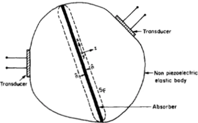
derived for two tranducers facing each other as follows: We consider two transducers, one used as transmitter and the other as the receiver as shown in Fig. 1. The Kino- Auld formula applies to this case directly. With the no- tation of Auld it can be stated as
6r
= ( 1 / 4 P )$
( v 1 * T2-
v2 T I )-
l i d s (1) where V is the particle velocity vector, T i s the stress ten-sor, ri is the inward directed normal to the surface S , sur- rounding the scatterer. The field quantities with subscript 1 are obtained when the left-hand side (LHS) transducer is excited with incident power P in the absence of scat- terer and those with subscript 2 are obtained when the right-hand side (RHS) transducer is excited with the same power in the presence of the scatterer. SF is a closed sur- face surrounding the scatterer, 6I’ is the change of the electrical transmission coefficient due to the presence of scatterer.
We assume that the scatterer consists of a highly ab- sorbing material with the same impedance as the propa- gation medium, therefore all the acoustic energy incident on it will be absorbed and nothing will be reflected. The scatterer is infinitely thin and planar. The coordinate sys-
tem is selected such that
z
= 0 plane is coincident with the scatterer. The surface SF is selected to be very close to the scatterer. For solution 1 (no scatterer, LHS trans- ducer excited) we have the same field quantities on both sides of SF: SF LHS O f SF: U J = V + TI = T + RHS of SF: V I = V + TI = T + .For solution 2 (with scatterer, RHS transducer excited) we have vanishing field quantities on the LHS of S,:
LHS of S F : ~2 = 0
T2 = 0 RHS of S F : 212 = V -
T2 = T -
where the superscripts show the direction of propagation of waves as well as the source of excitation. “
+”
and superscripts refer to waves propagating in+ z
and-z
direction, and excited by LHS and RHS transducers, lespectively. Since S, is parallel toz
= 0 plane, ii = a, and dS =dr
dy. Moveover, the transmission coefficient for solution 2 is zero. Therefore, (1) can be written as*‘-,P
-r
= (1/4p)+
( v I - T +-
+ T - ).
Ads SF( 2 )
Non piezoeleclrlc
Fig. 1. Scattering geometry used in formulation.
where is the electrical transmission coefficient from one transducer to the other in the absence of scatterer. This equation can be written more explicitly in terms of com- ponents of vectors and tensors as
r + w * + W
-r
= ( I / ~ P )J
J
(.TT;+
.;T;+
V ; T ;- W -m
- V : T , - v J T , - .:Ti)
dx
dy ( 3 )This equation is the same as [20, (3)] with different interpretation of superscripts. Hence the rest of the deri- vation is the same. The result for a homogeneous and isotropic propagation medium is
+
c44 k;+ m
ky”
+
k:2 -kxk, k X k:k:
+
k:2 kyk;ky k: k:
+
k ;!
where c,, and c44 are the elastic constants [21] of the isotropic medium; W is the operating frequency; P is the incident power;
CP
and \k are the Fourier transforms (hence angular spectra) of the scalar and vector potentials of the particle velocity field atz
= 0 plane. k, and k , are the wave vector components inx
and y directions. k z and kl614 IEEE TRANSACTIONS ON ULTRASONICS, FERROELECTRICS, AND FREQUENCY CONTROL, VOL. 35. NO. 5, SEPTEMBER 1988
( k , ) and shear waves ( k h ) as
Equation (4) expresses the transmission coefficient in terms of the angular spectra of scalar and vector potentials at a plane.
If we consider longitudinal waves only, (4) reduces to @ + m r + m
r
= ( ~ ~ ~ k ; / 8 ~ ~ ~ ~ )I-,
1
k Z @ - ( L kY>- m
9 + ( -kx, - k,) dk, dk, ( 5 )
where 9 + and @ - are the angular spectra of the acoustic waves at z = 0 plane generated by the LHS and RHS transducers, respectively. Equation ( 5 ) is a general for- mula that applies to two transducers. The z = 0 plane could be selected at any convenient location. This expres- sion can be reduced to that given by Johnson and Devaney
[22] except for the constant factors. A. Diffraction Loss for Isotropic Case
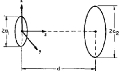
We can now return to the diffraction loss problem. Sup- pose that we have two longitudinal wave circular trans- ducers of radii a l and a2. The transducers are located
coaxially and facing each other at a distance d . The co- ordinate axes are selected as shown in Fig. 2. Assuming piston type transducers the scalar potentials,
41
and I $ ~ , at the plane of each transducer can be written as+ 1 ( ~ >
= circ [ ( x 2+
y 2 ) 1 ' 2 / a l ~4 2 @ )
= A2 circ[
(x2+
Y 2 ' / 2 ) /a21 where 1 r l lo
r > ~ ' circ ( r ) = Since P @ + mthe angular spectra at the same planes are [23]
@,(O) = 4a:Al jinc [(al/r)(kZ
+
k;)'/']a 2 ( d ) = 4a;A2 jinc [(a2/a)(kZ
+
k y ) 2 1/2]
where jinc ( x ) = J 1 ( ax)/2x and J1 is the first order Bes-
se1 function of the first kind. To be able to apply ( 5 ) an- gular spectra must be specified at the same plane. Prop- agating angular spectrum from one plane to the other is taken care of by a simple exponential phase factor [23], [24] :
42(0)
= 4a:A2 jinc [(a2/a)(k;+
k;) 1 /2]
exp ( - j k z d ) .X
Fig. 2 . Geometry and coordinate system for circular coaxial transducers separated by distance.
Applying ( 5 ) results in
jinc [(al/a>(k:
+
k;)1'2~jinc [(a2/a)(k;
+
/c;)'"]
dk, dk, ( 6 )Due to the circular symmetry the double integral of (6) reduces to a single integral:
4cll kia:a;AlA2 TWP
r =
S:"
k: exp ( - j k , d ) jinc [ ( a l / a ) ( k i - k:)'"]jinc [(a2/r>(ki
-
dkz (7)where the evanescent fields are neglected. Equation (7) can be rewritten as an inverse Fourier transform opera- tion:
( 8 )
where F-' is the inverse Fourier transform operator map- ping from k-domain to x-domain, and
If we assume transducers with zero conversion loss, we can relate the incident power and other parameters as
P = cllk:a:A:/w = c l , k o a 2 A 2 / w . 3 2 2
Hence (8) reduces to
rect ( k / k o - 1 / 2 )
.
ATALAR: CALCULATING DIFFRACTION LOSS BETWEEN TWO FACING TRANSDUCERS 615
Equation (9) expresses the transmission coefficient as a function of distance between the two transducers in the form of a one-dimensional Fourier transformation. The diffraction loss, L , can be easily deduced from L ( d ) =
-20 log I I ’ ( d ) ( .
B. Diffruction Loss for Anisotropic Case
Computing the propagation of bounded beams in an- isotropic media is in general involved. For this purpose, angular spectrum method can be employed [ 2 5 ] . Along or close to pure mode directions approximate methods sim- plify the problem greatly. To include anisotropy we as- sume that k , is small and following Papadakis [ 1 l] we will replace ko by k,( 1
+
be’) where 8 is the deviation angle of the k vector fromz
axis and b is the anisotropy factor as defined by Waterman. This approximation is valid even in the near field as long as term is negligible. For com- pleteness we repeat the expressions for anisotropy param- eter, b for various crystals and orientations: b = ( c 1 I -C12 - ~ C ~ ~ ) ( C I I
+
C I ~ ) / [ ~ ~ I I ( ~ I I-
C M ) ] for cubic SYS-tem
[loo]
propagation; b =+
c12+
c I I ) ( c I I+
2cI2+
q 4 ) / [ 3 ( c I 2+
c 4 4 ) ( c 1 1+
2c12+
4c44)] forcubic system [ l 1 l ] propagation; b = ( c33 - c13-
2 ~( c33 ~+
~ )c13)/[2c33(c33 - for hexagonal or tetragonal sys- tem c-axis, or trigonal system three-fold axis propagation.
Note that, for two-fold symmetry the b8’ formulation above does not apply, even though it may be a pure mode direction. With k : = k:
+
k : and for k , small, we may writeThis equation can be rearranged to give approximately
k f ( 1 - 2b)
+
k : = k i . Hencek , = ( k i - k ; ) /( 1 - 26)’’’
7 112
Therefore (7) must be changed to
* jinc
iinc
a
k
dk,f
( 1 1 ))
It is seen that effect of anisotropy is the same as changing the dimensions of the transducers. In other words, the dif- fraction loss will be the same for the following two cases:
Isotropic medium, circular transducers of size a l and
u2 separated by d .
Anisotropic medium, circular transducers of size
u l / ( 1 - 2b)’I2 and a z / ( 1 - 2 b ) ’ ” separated by d . One should note that above result is not valid in the near field if the O 4 term is no longer negligible.
C . Pulsed Excitation
The formula is valid for continuous wave signals, but it can be dependably used for pulsed systems where the pulse contains several cycles. For wide band systems,
Fourier analysis can be easily used to find the pulse re- sponse due to diffraction. Suppose that the input pulse can be represented by a time function, g ( t ) . Suppose also that the frequency spectrum of this time function is G( W ) with
G ( W ) = F { g ( t ) }
.
If the transducers can be assumed in- finite bandwidth, the pulse obtained at the other trans-ducer, h ( t ) , can be written as
h ( t ) = F - ’ ( G ( w ) q U ) } ( 1 2 )
where I’ ( U ) is the complex function that gives the trans-
mission coefficient as a function of frequency. 111. RESULTS
Evaluation of (9) requires the values of first order Bes- se1 functions. Bessel function can be calculated accurately and relatively fast using recurrence relations [26]. The in- verse Fourier transformation is done by the fast Fourier transform (FFT) algorithm [27]. Obviously, one must pay attention to aliasing effects during FFT operation. Be- cause the function inside the brackets of (9) is nonzero only within an interval, the sampling on the function can be done to include the entire FFT input range. The num- ber of points in the FFT must be large enough to reduce accuracy loss due to aliasing.
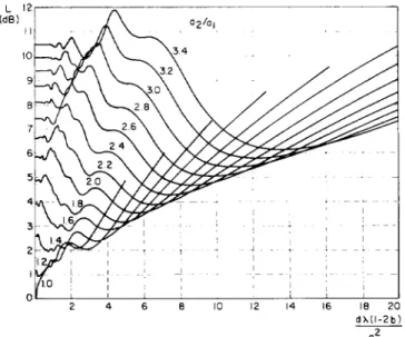
It is convenient to plot the diffraction loss as a function of normalized separation distance. A series of curves were obtained for various values of a, and u2. It was seen that the curves corresponding to different values of ul are
barely distinguishable from each other as long as u 2 / u 1
ratio remains the same. This simplifies the presentation of results. One set of curves is applicable to almost all cases. Fig. 3 and Fig. 4 are the plots of the results. The hori- zontal axis is the distance between the transducers and it is normalized with respect to .:/X, where X is the wave- length in the propagation medium. The normalization of the vertical axis is achieved with respect to u 2 / u l = 1
curve at d = 0 where the diffraction loss is zero. At d =
0 the calculated results for diffraction loss agree with the geometrical loss of 20 log ( a l / a 2 ) for u2
<
u l , and 20log ( a 2 / u l ) for u l
<
u 2 . The curves shown are for u I = 1 0 X but they are nearly independent of the value of u Iexcept when a , is very small. We have used a 8 196 point FFT in calculating the given curves’. The program had to be written in FORTRAN 77 due to the presence of com- plex numbers. The calculations took about 3 min per curve on an IBMiXT computer with 8087 numerical coproces- sor.
Since changing the frequency and changing the sepa- ‘Numerical results presented in [ZO. Fig. 41 do not agree with our pres- ent results, due to an error in numerical calculations there. With the error corrected same results are obtained.
616 IEEE TRANSACTIONS ON ULTRASONICS. FERROELECTRICS, AND FREQUENCY CONTROL. VOL. 35. NO. 5, SEPTEMBER 1988 1 , l I 2 3 I 4 d X ( I - Z b ) a:
Fig. 3 . Diffraction loss between circular transducers of radii and a , ( a , < a , ) separated by d i n anisotropic medium with anisotropy parameter b .
I 12, . -. l
Fig. 4. Diffraction loss between circular transducers of radii U , and a z ( a r
> a , ) separated by d i n anisotropic medium with anisotropy parameter b .
ration are equivalent, the same set of curves can be used for pulse response determination. In this case horizontal axis of Figs. 3 and 4 becomes the inverse frequency axis, and curves shown become F ( 1 / U ) of (12). One also
needs the phase of the transmission coefficient for this purpose. Fig. 5 and Fig. 6 are the calculated excess phase curves. The phase curves start at zero and approach 7r/2
asymptotically. They are pretty smooth in the far field meaning that there will be very small pulse distortion. In the near field and especially when the ratio of transducers is large, the phase curves loose the smoothness thus caus- ing pulse distortion.
For the case a l = u2 the problem can be reduced to a single transducer geometry with a perfect and parallel re-
Fig. 5. Excess phase of transmission coefficient between circular trans- ducers of radii a , and a 2 ( a 2 < a , ) separated by d i n anisotropic medium with anisotropy parameter b. Curves are displaced from each other ver- tically for clarity.
Excess n, I
Fig. 6. Excess phase of transmission coefficient between circular trans- ducers of radii U , and a2 ( a , > a , ) separated by d in anisotropic medium wlth anisotropic parameter B . Curves are displaced from each other ver- tically for clarity.
flector at a distance d / 2 . For this case, given amplitude and phase curves are in good agreement with previous cal- culations and experimental results [l l], [ 121.
For the anisotropic case the only thing that needs to be changed is the scaling of the horizontal axis. In this case horizontal axis label is changed to d X ( 1
-
2 b ) / u : .Therefore, we may add one more case to the equivalent diffraction loss cases mentioned in the previous section: anisotropic medium, circular transducers of size u l and u2
separated by d / ( 1 - 2 b ) .
ATALAR: CALCULATING DIFFRACTION LOSS BETWEEN TWO FACING TRANSDUCERS 617 Papadakis [ 1 l ] a s well as Cohen and Gordon [ 141 for the
case a , = a2. If anisotropy factor b is positive the sepa- ration between the transducers can be increased without changing the diffraction loss. On the other hand, if b is
negative the separation should be reduced to keep the same diffraction loss.
Inspection of Figs. 3 and 4 indicates that except when the values of a l and a2 are very close to each other, the minimum diffraction loss is achieved when the two trans- ducers are separated by a finite distance. This distance is slightly higher than the Fresnel distance ( a 2 / X ( l - 2b))
of the larger transducer. This distance is at a point where the acoustic field produces a waist [l]. On the other hand, for a 2 / a , = 0.7 the diffraction loss remains nearly the same at about 2.5 dB when d is less than 2 a : / X ( l - 2 b ) .
In all cases, when the separation distance gets very large, the diffraction loss increases by 6 dB per doubling of dis- tance.
As an example of use of the plots consider an acoustic
lens design at 2 GHz. The radius of the lens cavity is to be 40 pm on one side of a 1 mm long sapphire rod. With
50” half-opening angle the pupil radius becomes 30.6 pm. The problem is the determination of optimal transducer size for minimum diffraction loss. With a , = 30.6 pm,
X
=
5.55
pm, d = 1000 pm and b = 0.16 (for sapphire[21]) we have dX( 1
-
2b)/a: = 4.03. Inspection in Fig.4 indicates that minimum diffraction loss is achieved when
q / a , = 1.4, or a2 = 43 pm. For this case diffraction loss is about 2.5 dB. The same problem in quartz ( X = 3.18.
b = -0.23, dX( 1 - 2 b ) / a : = 4.97) results in a trans- ducer radius of 49 pm and a loss of 3 dB. If one uses a 2- mm long sapphire rod, optimum transducer size and dif- fraction loss become 67 pm and 4.2 dB, respectively. In all cases, the total diffraction loss in the acoustic lens ele- ment will be twice the found values because of two-way propagation.
Note that in the acoustic lens design, minimization of diffraction loss may not be the only criterion. If uniform illumination of lens is desired for the purpose of higher resolution, one may deviate from the transducer sizes given above at the cost of higher diffraction loss.
IV. CONCLUSION
We have presented a fast method of calculating diffrac- tion loss between two transducers in isotropic or aniso- tropic media along or close to pure mode directions. Given graphs are in complete agreement with previous theoret- ical and experimental results for the limiting case of equal transducer sizes. They enable the determination of dif- fraction loss and excess phase between two coaxial cir- cular transducers or of optimum transducer size for min- imum diffraction loss. The same graphs can be used for predicting the pulse response. The theory developed is general: the transducer shape is not limited to circular ge- ometry; one can easily adopt other transducer shapes. The plots given in this paper make the design of acoustic lenses to be used in scanning acoustic microscopes a simple task.
REFERENCES
[ l ] J . Zemanek, “Beam behavior within the nearfield of a vibrating pis- ton,‘’ J . Acoust. Soc. Am., vol. 49, no. l, pp. 181-191, 1971. [2] J. C. Lockwood and J. G. Willette, “High-speed method of comput-
ing the exact solution for the pressure bariations in the nearfield of a baffled piston.” J . .4cousr. So<,. Art!. , vol. 53, no. 3 , pp. 735-741, 1973.
[3] P. R. Stephanishen. “Transient radiation from pistons in an infinite planar baffle,” J . AcouJr. Soc. Am., vol. 49. no. 5, pp. 1629-1618. 1971.
[4] W . L. Beaver, “Sonic nearfields of a pulsed piston radiator.” J .
Acousr. Soc. Am., vol. 56. no. 4. pp. 1043-1048, 1974.
[ 5 ] G. R . Harris, “Review of transient field theory for a baffled planar piston.” J . Acoust. Soc. A m . . vol. 70. no. 1. pp. 10-20, 1981.
[ 6 ] J . N . Tjotta and S. Tjotta. “Nearfield and farfield of pulsed acoustic radiators,” J. Acoust. Soc. Am., vol. 71. no. 4 , pp. 824-834,
1982.
[7] D. Guyomar and J . Powers, “Transicnt fields radiated by curved sur- faces-Application to focusing,” J . Acoust. Soc. ,4m.. vol. 76, no. 5, [S] W. L . Nyborg and R. B. Steele, “Nearfield of a piston source of ultrasound i n an absorbing medium,” J . Acousr. Soc. A m . , vol. 78, pp. 1882-1891. 1985.
[9] D. A. Hutchins. H. D. Mair, P. A. Puhach and A. J. Osei, “Contin-
uouh-wave pressure fields of ultrasonic transducers,” J . Acouct. Soc.
A m . , vol. 80. no. I . pp. 1-12, 1986.
[ I O ] H. Seki, A . Granato, and R . Ttuell. “Diffraction effects in the ultra- sonic field of a piston source and their importance in the accurate measurement of attenuation,” J . Acoust. Soc. A m . , vol. 28, no. 2. [ I I ] E. P. Pdpadakis, “Ultrasonic ditl’ractlon loss and phase change in anisotropic materials,” J . Acoust. Soc. A m . . vol. 40, no. 4, pp. 863- 876, 1966.
[l21 -. “Ultrasonic phase velocity by the pulse-echo-overlap method incorporating diffraction phase correction.” J . Acousr. Soc. A m . , vol. 4 2 , no. 5 , pp. 1045-1051, 1967.
[l31 -, “Ultrasonic diffraction from single apertures with appl~cation to pulse measurements and crystal physics,” in Physical Acousticx.
W . P. Mason and R . N . Thurston. Eds. New York: Academic, 1979,
[ 141 M . G . Cohen and E. L. Gordon, “Focusing of microwave acoustic
beams.” J . Appl. Phys., vol. 38. no. 5 , pp. 2340-2344, 1967.
[l51 M. B. Gitis and A . S. Khimunin. “Diffraction effects in ultrasonic measurements (Review),” Sov. Phys-Acousr., vol. 14, no. 4, pp. [l61 P. C . U‘aterman, “Orientation dependence of elastic waves in single
crystals,” Phvs. Rev., vol. 113, no. 5 . pp. 1240-1253, 1959.
1171 C . F. Quate. A. Atalar and H . K . Wickramasinghe, “Acoustic mi- croscopy with mechanical scanning-A review,” Pmc. I E E E , 1979, vol. 67, pp. 1092-1 114.
1181 G . S . Kino. “The application of reciprocity theory to scattering of acoustic waves by flaws,” J . Appl. Phys., vol. 49. no. 6. pp. 3190- 3199, 1978.
[ 191 B. A. Auld, “General electromechanical reciprocity relations applied to the calculation of elastic wave scattering coefficients,” Wuve Mo- rion, vol. l , no. l , pp. 3-10, 1979.
[20] A. Atalar, “ A backscattering formula for acoustic transducers,” J .
Appl. P h y s . , vol. 5 1 . no. 6 . pp. 3093-3098, 1980.
[21] B . A. Auld, Acoustic Fields and Waves in Solids, vol. 1. New York: John Wiley and Sons, 1973.
1221 R. K. Johnson and A. J . Devaney. “Transducer effects i n acoustic scattering measurements,” Appl. Phys. Lett.. vol. 41, no. 7, pp. 622-
624, 1982.
I231 J . Goodman, Introduction ro Fourier Optics. New York: McGraw- Hill, 1968.
[24] A . J. Devaney and G . C . Sherman. “Plane-wave representations for scalar wave fields,” SIAM Rev., vol. 15, pp. 765-786, 1973.
[25] D. J . Vezzetti, “Propagation of bounded ultrasonic beams i n aniso- tropic media,” J . Arousr. Soc. Am., vol. 78, no. 3 , pp. 1103-1 108, 1985.
[26] M . Abromowitz and I. A . Stegun. Handbook qfMurhemuricul Func- tions. New York: Dover, 1970. p. 385.
[27] E. 0 . Brigham. The Fust Fourier Transform. Englewood Cliffs, N.J.: Prentice Hall, 1974.
pp. 1564-1572, 1984.
pp. 230-238, 1956.
vol. 12, pp. 151-211.
618 IEEE TRANSACTlONS ON ULTRASONICS, FERROELECTRICS, AND FREQUENCY CONTROL, VOL. 35, NO. 5, SEPTEMBER 1986
Abdullah Atalar was born in Gaziantep, Turkey, in 1954. He received the B.S. degree from Middle East Technical University, Ankara. Turkey in 1974, and the M . S . and Ph.D. degrees from Stan- ford University, Stanford, CA, in 1976 and 1978, respectively, all in electrical engineering. His the- sis work was on reflection acoustic microscopy.
From 1978 to 1980 he was first a Post Doctoral Fellow and later an Engineering Research Asso- ciate at Stanford University, he continued his work on acoustic microscopy. For eight months he was with Hewlett Packard Labs, Palo Alto, CA, engaged in photoacoustics re-
search. In 1980 he joined the Middle East Technical University as an As- sistant Professor. From 1982 to 1983 on leave from University, he was with Ernst Leitz Wetzlar, Wetzlar, West Germany, where he was involved in the development of the commercial acoustic microscope. He is presently an Associate Professor and chairman of the Electrical and Electronics En- gineering Department at Bilkent University and is a part-time faculty mem- ber at Middle East Technical University. His current research interests in- clude acoustic imaging, linear acoustics, and computer-aided design in Electrical Engineering.
Dr. Atalar is a member of Chamber of Electrical Engineers of Turkey. In 1984 he was given the H. TugaC Foundation Award of TUBITAK, Tur- key for his contributions to acoustic microscopy.