Physical optics modeling of 2D dielectric lenses

Physical optics modeling of 2D dielectric lenses

Vladimir B. Yurchenko1,*and Ayhan Altintas2

1

Institute of Radiophysics and Electronics, National Academy of Sciences of Ukraine, 12 Proskura St., 61085 Kharkov, Ukraine

2_{Electrical and Electronics Engineering Department, Bilkent University, 06800 Bilkent, Ankara, Turkey}

*Corresponding author: [email protected]

Received August 20, 2008; revised December 8, 2008; accepted December 8, 2008; posted December 11, 2008 (Doc. ID 100392); published January 27, 2009

We propose an advanced physical optics formulation for the accurate modeling of dielectric lenses used in quasi-optical systems of millimeter, submillimeter, and infrared wave applications. For comparison, we obtain an exact full-wave solution of a two-dimensional lens problem and use it as a benchmark for testing and vali-dation of asymptotic models being considered. © 2009 Optical Society of America

OCIS codes: 080.3630, 110.6795, 220.3630, 260.1960.

1. INTRODUCTION

An accurate design of large-scale quasi-optical systems with dielectric lenses requires advanced wavelike asymptotic modeling of refractive components. An ex-ample of such a system is QUaD, a submillimeter-wave telescope for cosmic microwave polarization measure-ments [1]. For this high precision instrument to be real-ized, extremely accurate modeling of aberrations is needed with further minimization of their effects. The problem is particularly challenging when polarization in the focal domain has to be computed [2]. In this case, with no exact solution available due to the size limit, there is a need of advanced asymptotic methods for the wavelike modeling of lenses similar to the physical optics simula-tions of large reflectors [3].

Other applications for the wavelike asymptotic model-ing of lenses may include optics for infrared and terahertz imaging (e.g., in security checks), automotive radars for collision-avoidance systems (where, specifically, cylindri-cal lenses are being used [4]), special microlenses for op-tical recording devices [5–8], etc.

When developing asymptotic methods, comparisons with exact solutions are of importance. In the meantime, an exact solution for electromagnetic scattering by a di-electric body is a complicated problem when the body is of a large electrical size. There are various approaches to the problem ranging from the finite difference, finite ele-ments, and similar methods [9] to sophisticated formula-tions based on the integral equaformula-tions [10,11] combined with regularization techniques [12–14]. Exact methods are usually limited to systems of small size, often less than ten wavelengths in diameter even in those cases when advanced solvers are available (e.g., ANSOFT HFSS

software). Besides, there is only a limited number of exact solutions for dielectric lenses described in the literature.

One example of a full-wave solution is the modeling of a microcylindrical axilens [6] by using the integral equa-tions [11] with no regularization. A rigorous regulariza-tion method [13,14] is proposed for the body of special ge-ometry considered as a resonator. A promising hybrid

technique is developed for diffractive microlenses [5], where the finite difference method solves the problem in the near field and the partial plane wave (PW) propaga-tion is used to transform the solupropaga-tion to the far field.

However, there appears to be no exact solutions pub-lished for conventional lens geometries, e.g., for a com-mon biconvex lens of a standard shape. Similarly, there are no wavelike asymptotic methods developed for lenses that outperform simulations based on the ray tracing ap-proach [2]. Conventional wave theory of lenses [2] is, in fact, the paraxial Fourier-optics, where nonparaxial cases are classified as a standing problem. The same paraxial limitations and related approximations (scalar waves, etc.) lay in the basis of quasioptical simulation models [1] that, therefore, do not account for polarization effects and nonparaxial issues in the interaction of the vector electro-magnetic waves with the dielectric lens body.

In the meantime, lenses of intermediate (quasi-optical) size (tens to a few hundreds of radiation wavelength) do, usually, require both the large-angle incidence and the vector character of the electromagnetic field to be ac-counted for while being too large for exact simulations. It is this kind of lens enhanced asymptotic modeling that is required for emerging practical applications.

The aim of this paper is to present enhanced asymptotic simulation methods for dielectric lenses of the quasioptical range and to provide validation for these methods by comparing them with full-wave analytic solu-tions obtained for two-dimensional (2D) focusing lenses of a conventional biconvex profile.

In Section 2, we obtain a full-wave analytic solution to the problem of an electromagnetic wave being focused by a 2D dielectric lens with a typical cross section profile formed by two circular arcs as shown in Fig.1. In this so-lution, we consider the cases of PW and cylindrical wave (CW) incidence on the lens surface and compute the wave fields behind the lens for two orthogonal polarizations, TE and TM, respectively. Then, in Section 3, we describe asymptotic methods appropriate for quasi-optical lenses that utilize the physical optics approach. Finally, we

pare simulation results produced by asymptotic methods with exact solutions at various values of lens parameters.

2. FULL-WAVE SIMULATION OF A

TWO-DIMENSIONAL FOCUSING

DIELECTRIC LENS

A. Simulation Method

Full-wave analytic solutions for dielectric lenses in the 2D problems shown in Fig.1can be obtained by direct meth-ods when using CW expansions of incident and scattered fields with respect to O1 and O2 frames associated with

circular arcs S1Land S2Lthat form the lens cross section

profile.

The lens geometry is defined by the lens diameter D and the arc curvature radii R1,2so that the lens angular

half-size ␪1,2 as viewed from the origin O1,2 is ␪1,2

= arcsin共D/2R1,2兲, the distance between the origins is L

= R1cos共␪1兲+R2cos共␪2兲, and the lens thickness along the x-axis is t = R1+ R2− L.

In this paper, we consider the waves of TE_共H储zˆ_{兲 and}

TM 共E储zˆ兲 polarization with two kinds of wave sources,

namely, the uniform PW and CW incident on the lens from the left (Fig.1). The incident wave in the PW case propagates along the positive direction of the x-axis. In the CW case, the incident wave is radiated from a line source located at a certain distance in front of the lens. In the xy plane, it is an omnidirectional source placed at the

xC, yCpoint on the left side of the lens with xC⬍−R1 and yC= 0 being the source coordinates in the O1 frame (the

left and right apex points of the lens have coordinates

xL= −R1and xR= −R1+ t, respectively).

Using the O1 frame, we expand the relevant z-component of the field (U = Ez in the TM cases and U

= Hzin the TE cases) in cylindrical functions in the

do-mains D1e, D1i, and DLas follows:

U =

兺

n 关AnJn共kr1兲 + BnYn共kr1兲兴ein␾1, 共r1,␾1兲 苸 DL, 共1兲 U =

兺

n CnJn共kr1兲ein␾1, 共r1,␾1兲 苸 D1i, 共2兲 U =

兺

n 关FnHn共kr1兲 + bn共kr1兲兴ein␾1, 共r1,␾1兲 苸 D1e, 共3兲

where An, Bn, Cn, and Fnare the unknown expansion

co-efficients, Jn共·兲, Yn共·兲 and Hn共·兲=Hn共2兲共·兲 are the Bessel,

Neumann, and Hankel functions of order n (the time de-pendence of the wave field is assumed to be exp共i␻t兲), k = 2␲/␭ and kd= k

冑

␧ are the wavenumbers in free space

and in the lens dielectric material of (complex) relative permittivity ␧, respectively, ␭ is the free-space wave-length, r1and ␾1are the radial and angular coordinates

in the O1frame, R1and R2are the curvature radii of the

entrance_共S1L兲 and exit 共S2L兲 lens surfaces, and the

ex-pansion domains are defined as D1e,2e=兵r1,2: r1,2⬎R1,2其, D1i,2i= D1,2− DL, D1,2=兵r1,2: r1,2⬍R1,2其, and DL= D1艚D2.

The expansions satisfy the Helmholtz equations in the relevant domains and boundary conditions of (a) no sin-gularity at the origin (there is neither source nor sink at point O1) and (b) no incoming waves from infinity except

the given source wave (the radiation boundary condition). The terms bnrepresent the source wave and take on the

form bn共kr1兲=i−nJn共kr1兲 in the PW case and bn共kr1兲

=共−1兲n_J

n共kr1兲Hn共kLC兲 in the CW case, where LC=兩CO1兩 is

the distance from the source point C to the frame origin

O1 (the source distance from the lens front surface is LCL= LC− R1).

The Neumann addition theorem for cylindrical func-tions is used for transforming the expansions from one frame共O1兲 to another 共O2兲 when imposing boundary

con-ditions for tangential field components at the lens sur-faces S1Land S2L. Then, by using the orthogonality of

an-gular harmonics, we arrive at the set of linear algebraic equations with respect to expansion coefficients as fol-lows:

兺

n,m 兵关AnJm−n共kdL兲 + BnYm−n共kdL兲兴Jm共kdR2兲 − CnJm−n共kL兲Jm共kR2兲其Smp共␪2兲 = 0, 共4兲

兺

n,m 兵␩关AnJm−n共kdL兲 + BnYm−n共kdL兲兴Jm⬘共kdR2兲 − CnJm−n共kL兲Jm⬘共kR2兲其Smp共␪2兲 = 0, 共5兲

兺

_n 兵关AnJn共kdR1兲 + BnYn共kdR1兲兴Pnp共␶兲 + CnJn共kR1兲Snp共␶兲其 − FpHp共kR1兲 = bp共kR1兲, 共6兲

兺

_n 兵␩关AnJn⬘共kdR1兲 + BnY⬘n共kdR1兲兴Pnp共␶兲 + CnJn⬘共kR1兲Snp共␶兲其 − FpHp⬘共kR1兲 = bp⬘共kR1兲, 共7兲 x O S 2 1L 2L D D D 1i 1e D D L θ2 2i 2e R 2 _R 1 θ1 S 2v S 1v S D y L O 1

Fig. 1. Geometry of a 2D convex dielectric lens (cross section profile). The excitation wave (PW or CW) of either TM共E储zˆ兲 or TE共H储zˆ兲 polarizations is incident from the left.

where p = 0 , ± 1 , . . ., Smp共␪兲=sin关共m−p兲␪兴/关␲共m−p兲兴 if m

⫽p, Smp共␪兲=␪/␲ if m=p, Pnp共␶兲=␦np− Snp共␶兲, ␶=␲−␪1, ␩

=

冑

␧ in TM and␩= 1 /

冑

␧ in TE polarizations, and prime 共

⬘

兲 denotes the derivative of a function over argument. By introducing reasonably large truncation numbers N and

M for summations in n and m, respectively, we could find

sufficiently convergent numerical solutions to Eqs.(4)–(7)

that, by substitution into Eqs.(2) and (3), allowed us to compute fields in the focal domain behind the lens.

Because of rapid growth or decay of cylindrical func-tions with angular harmonic index n, direct solufunc-tions of this kind are limited to lenses of relatively small size (truncation numbers have to be limited from above). In practice, we could simulate lenses with the curvature ra-dii R1, R2, and lens diameter D up to about 12␭ when

hav-ing the lens refractive index n˜ = 1.5 (notice, the lenses

used in, e.g., car radar applications [4] are of a similar size D⬇10␭). A further increase of the lens size can be achieved by implementing regularization methods.

B. Simulation Results

The results showing the wave focusing effects in TM and TE polarizations for both the PW and the CW incident

fields are plotted in Figs.2and3. We choose the lens re-fractive index n˜ = 1.5 so that, in the case of PW incidence,

the geometrical focal point F1of a thin symmetric lens

co-incides with the frame origin O1(the case of PW incidence

was examined in detail in our earlier work [15]).

Power density Pz=兩Uz兩2associated with Ezand Hzfield

components of TM and TE waves, respectively, is shown in the focal domain of lens in transverse共y兲 and longitu-dinal共x兲 cuts passing through the focal point F1. A

com-mon feature of these and other simulations is that the TE polarized waves produce a greater power density at the focal point as compared to the TM waves of the same in-cident power. This is due to the difference in TE and TM wave transmissions at oblique incidence at the lens sur-faces as expressed by the Fresnel coefficients. The effect is more complicated for small lenses and CWs [Fig. 3(a)], though, typically, it remains of a similar kind.

The second common feature is that the width of the fo-cal spot defined as the distance between the first minima of the field is twice the wavelength in all the cases of PW focusing [Fig.2(b)]. In the meantime, the width of diffrac-tion fringes is one wavelength for lenses of a different size with nearly identical patterns in both polarizations. In

0 2 4 6 8 10 12 14 -10 -8 -6 -4 -2 0 2 4 6 8 10 Pz x A B

(a)

0 2 4 6 8 10 12 14 -10 -8 -6 -4 -2 0 2 4 6 8 10 Pz y A

(b)

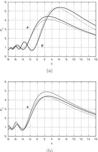
Fig. 2. Exact (solid curves) and asymptotic solutions (dashed curves for RS2 and dotted curves for KU models, see below) in the case of TM PW incidence on a symmetric 2D dielectric lens; (a) x and (b) y cuts of Pzpower distribution behind the lens. Here, n

˜ = 1.5, R1= R2= D,␪1=␪2= 30°; A and B groups of curves

corre-spond to D = 12_{␭ 共xR}= −8.7_{␭兲 and D=6␭ 共xR}= −4.3_{␭兲, respectively.}

0 1 2 3 4 5 6 -8 -6 -4 -2 0 2 4 6 8 10 12 14 16 Pz x A B

(a)

0 1 2 3 4 5 6 -8 -6 -4 -2 0 2 4 6 8 10 12 14 16 Pz x A

(b)

Fig. 3. (a) Exact solutions in TE (solid curves) and TM (dotted curves) cases of CW incidence on a lens with R1= 10␭ when (A) D = R₂= 8_{␭ 共xR}= −8.0_{␭兲 and (B) D=R2}= 10_{␭ 共xR}= −7.2_{␭兲 at LC} = 30_{␭ (LCL}= 20_{␭, n˜=1.5) and (b) comparison of exact (solid curve)} and asymptotic solutions (dashed curves for RS2 and dotted curves for KU models, see below) in case A of TE CW incidence.

the case of CW focusing, the focal spot is, typically, wider and the focusing effect is more complicated (see below).

In general, there are some intrinsic resonant effects as-sociated with lenses, which are especially pronounced in the narrowband applications. With increasing the size of the lens and the bandwidth of radiation, the resonant ef-fects smear out and become insignificant (especially in the presence of losses).

3. ASYMPTOTIC WAVELIKE MODELING OF

DIELECTRIC LENSES

A. Two-Term Kirchhoff Approximation

Asymptotic approximations proposed in this paper are based on various forms of diffraction integrals that repre-sent wave propagation from the lens exit surface to the observation points behind the lens. The integral trans-forms of this or a similar kind are needed in any near-field to far-near-field propagation in free space.

Inside the lens, propagation of the incident wave from the entrance surface S1L to the exit surface S2L can be

evaluated by using the ray tracing through the lens body. In this paper, the ray tracing is implemented on account of (a) the transmission Fresnel coefficients at S1Land S2L

surfaces, (b) phase increments along the rays inside the lens, and (c) wave amplitude increments (decrements) due to the ray convergence (divergence) because of refrac-tion. This evaluation is quite accurate for typical lenses because of a relatively short ray propagation path inside the lens as compared to the lens transverse dimensions.

The first method we consider is based on the two-term Kirchhoff diffraction integral. The integral is evaluated over the extended exit surface S2that consists of the lens

exit surface S2Land the free-space surface S2F extended

from the lens rim to infinity in the transverse direction. The first term depends on the wave amplitude U that is directly evaluated at the exit surface S2 as explained

above. The second term depends on the normal derivative of U at S2that is approximated by using the U values at S2and the set of ray directions that define the local

incli-nation of the wavefront (we denote this approach as the KU model).

B. One-Term Rayleigh–Sommerfeld Formulation Modified for Curved Surfaces

Another asymptotic model is obtained by starting with a one-term Rayleigh–Sommerfeld diffraction integral and modifying it for nonplanar (curved) exit surfaces. Since the idea of the original Rayleigh–Sommerfeld formulation is the choice of the Green’s function that vanishes at the plane integration surface (thus removing the second poorly defined term in the Kirchhoff formulation), we fur-ther modify the Green’s function to make it identically zero at the curved lens exit surface S2L while using the

original form at the planar free-space surface S2Foutside

the lens. We denote this formulation as an RS2 model. Notice, the Green’s function defined above is an exact one for the domain of a given geometry. It means that, if the field on the exit surface S2is known precisely, the

for-mulation is exact. Therefore, the RS2 model is superior to other forms of the Rayleigh–Sommerfeld approach pro-posed for curved surfaces as, e.g., those where no

modifi-cation of the Green’s function is made [7] or an alternative four-term Green’s function is introduced [8] that, how-ever, generates entirely wrong results when tested in our simulations.

C. Comparison of Exact and Asymptotic Solutions

An important goal of this paper is the validation of asymptotic models by comparing their results one with another and with available exact solutions when consid-ering various kinds of lenses. Therefore, we examine the performance of asymptotic models and relevant software codes in a broad domain of lens parameters.

The comparison of KU and RS2 simulations with full-wave solutions is presented in Figs.2 and3(b). In these cases, the lenses are characterized by the focal length f ⬃D⬎␭. In these and other simulations [15], KU and RS2 models appeared to be, in general, sufficiently accurate.

Inaccuracy in asymptotic models may arise due to (a) neglect of the edge diffraction and the internal reflection in the lens, (b) inaccuracy of the ray model for the wave propagation inside the lens, (c) approximations in the am-plitude and phase evaluation of the wave transmitted through the lens exit surface, and (d) additional approxi-mations in the KU model needed for the evaluation of a normal derivative of the wave field at the lens exit surface

S2L.

A typical feature observed in asymptotic solutions is that the values of power density Pz共x,y兲 computed with

KU and RS2 models provide the lower and the upper bounds for the exact solution, respectively. Therefore, by combining both the KU and RS2 results, we can, gener-ally, estimate and improve the accuracy of approximate asymptotic simulations.

Capabilities of asymptotic models in computing 2D field distributions are shown in Fig.4. Figure4(a)shows an exact power pattern (in relative units) in the focal do-main of the lens presented in case B of Fig.3in TE polar-ization (CW excitation by the line source at LC= 30␭ when

D = R1= R2= 10␭). One can see a pair of specific fringes

originating at the lens rim due to the edge diffraction (the waves aside the lens are partially suppressed by this ef-fect near the lens rim). The lens is suspended freely in space as shown in Fig.1.

Figure 4(b)shows the pattern computed for the same lens with the RS2 asymptotic model.There is a clear simi-larity between the patterns in Figs.4(a)and4(b)in all the main features, such as the focal spot, basic diffraction fringes in the focal domain, two rather bright caustics, and even a specific interference structure along the caus-tics consistent with fringes behind the lens. A noticeable difference is only the absence of significant edge diffrac-tion and no suppression of waves aside the lens, respec-tively (there is no special account for edge diffraction in this model yet).

In practice, the lens is usually mounted into a stop that is not transparent for the incident waves. The stop is not accounted for by an exact solution described above. The asymptotic models can, however, easily account for the stop. Figure 4(c) shows the pattern computed with the RS2 model for the same lens as described above, which is mounted into the stop. The stop is simulated as an ab-sorbing screen orthogonal to the x-axis with an aperture

of size D where the lens is fixed by its rim. The pattern shows significant suppression of the side waves behind the screen except those diffracted by the lens, though all the wave features in the focal domain are the same as in Figs.4(a)and4(b).

D. Asymptotic Solutions for Large- and Small-Scale Lenses

Asymptotic approximations should be particularly useful for large-scale lenses, where exact solutions are not acces-sible while asymptotic methods remain efficient. Gener-ally, short-wave asymptotic methods are more accurate for large scattering objects as compared to small ones. The rule is valid for dielectric lenses as well, though in this case, there are two kinds of parameters that control the accuracy, namely, (a) the lens surface curvature radii

Ri and (b) their ratio to the lens diameter (equivalently,

the lens aperture angles␪i) rather than the lens diameter

D alone.

The discrepancy between KU and RS2 models de-creases with increasing the size of the lens of the same profile. For example, the discrepancy in Pz at the focal

point of a rather bulky symmetric lens in case A of Fig.

2(a)decreases from nearly 25% when D = R1= R2 = 12␭ to

10% and 5% for a lens of the same shape at D = R1= R2

= 100␭ and D=R1= R2 = 300␭, respectively. Yet, the

dis-crepancy for bulky lenses such as this共t/D=0.27兲 is rela-tively significant, being the consequence of general diffi-culty in solving large-angle共␪1=␪2= 30°兲 nonparaxial lens

problems [2]. 0 2 4 6 8 10 12 -100 -80 -60 -40 -20 0 20 40 60 80 100 Pz x A B

(a)

0 5 10 15 20 25 30 35 40 45 -100 -80 -60 -40 -20 0 20 40 60 80 100 Pz x A B

(b)

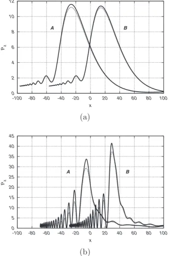
Fig. 5. Power density P_z(TM PW case) in the focal domain of asymmetric lenses of diameter (a) D = 30_{␭ and (b) D=90␭ 共n˜} = 1.5兲 when either R1= 100␭, R2= 60␭ (A orientation of lens), or R1= 60␭, R2= 100␭ (B orientation) computed with KU (dotted

curves) and RS2 (solid curves) asymptotic methods. Fig. 4. Power patterns Pz共x,y兲 behind the lens in case B of Fig.

3in TE CW incidence. (a) Exact solution for a lens suspended in free space, (b) RS2 simulation for the same case, and (c) RS2 simulation for the same lens mounted into a stop.

Another example is presented in Fig. 5, which com-pares the effects in relatively thin and thick asymmetric lenses of a sufficiently large scale. It shows the power density Pz(TM PW case) in the focal domain of

asymmet-ric lenses of diameter (a) D = 30␭ and (b) D=90␭ when ei-ther R1= 100␭, R2= 60␭ (A orientation of lens), or R1

= 60␭, R2= 100␭ (B orientation) computed with KU and

RS2 methods (these are relatively large lenses with focal length f⬎DⰇ␭ that cannot be easily simulated by exact methods).

Figure 5(a) illustrates a good agreement (better than 2%) of asymptotic methods for a lens of a limited diameter 共D=30␭兲 in the case of relatively large radii R1,2 when

␪1= 8.6°,␪2= 14.5° (in B orientation) and the lens

thick-ness is t = 3␭. In the meantime, Fig.5(b)shows quite a sig-nificant discrepancy between asymptotic methods (up to 10%) when the lens diameter is three times greater共D = 90␭兲 at the same radii R1,2 as before. In this case,␪1

= 48.6°,␪2= 26.7°, and the lens thickness t = 31␭ (the

rela-tive lens thickness is t / D = 0.10 and t / D = 0.34 in Figs.5(a)

and 5(b), respectively). Figure 5(b) also shows a certain advantage of the B orientation of large asymmetric lenses for obtaining a sharper focusing of incident PWs.

E. Optimal Asymptotic Approximations for Asymmetric Lenses

The results above are obtained for symmetric or slightly asymmetric lenses that have comparable surface curva-ture radii R1⬃R2. For asymmetric lenses with R1ⰇR2

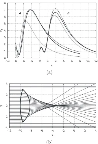
and a relatively small focal length 共f⬃D⬃10␭兲 we ob-serve, however, certain problems. For these lenses, the re-sults of two asymptotic methods may differ significantly [Fig.6(a)dashed and dotted curves in case A]. The effect is less pronounced for greater lenses of a similar shape, though the tendency remains the same.

A detailed analysis revealed that, in these cases, we ob-serve the effect of total internal reflection of rays near the lens rim. Due to this effect, no wave can propagate through the lens in the rim area [Fig.6(b)]. Moreover, the area near the rim where the wave would experience total internal reflection may be quite significant. Notice, even though both the KU and the RS2 models take account of this effect by assigning zero amplitude to the wave in this area on the exit surface S2L, inconsistency of approximate

field distributions (and also of a normal derivative in the KU model) in this domain may be much too significant for certain models to be reliable.

To compare the applicability of different models for asymmetric lenses, we computed exact solutions in those

0 1 2 3 4 5 6 7 8 -10 -8 -6 -4 -2 0 2 4 6 8 10 12 Pz x A B

(a)

-4 -2 0 2 4 -12 -10 -8 -6 -4 -2 0 2 4 y x

(b)

Fig. 6. (a) Power density Pz(TE PW case) in the focal domain of

an essentially asymmetric lens of small size in A and B orienta-tions (n˜ = 1.5, D = 6_{␭, R}1= 10␭, R2= 4␭ in case A when ␪1

= 17.5° ,␪₂= 48.6°) computed with KU (dotted curves) and RS2 (dashed curves) asymptotic methods as compared to exact solu-tions (solid curves), and (b) total internal reflection near the lens rim in case A as illustrated by ray tracing (a few rays near the rim in this plot do not propagate through the lens).

0 1 2 3 4 -4 -2 0 2 4 6 8 10 12 14 Pz x ( y = 0 ) , y ( x = xF) A B

(a)

-8 -4 0 4 8 -8 -4 0 4 8 12 16 20 24 y x

(b)

Fig. 7. (a) Power density Pz共y兲 at x=xF(A curves) and Pz共x兲 at y = 0 (B curves) computed by KU (dotted curve) and RS2 (dashed

curve) asymptotic methods in the comparison with an exact so-lution (solid curve), and (b) set of rays in the case of CW inci-dence on an asymmetric lens in the B orientation when D = 8_␭,

cases where it was possible [Fig.6(a)solid curves]. It ap-pears that exact solutions are also quite difficult to obtain in those cases when the effect of total internal reflection is observed.

The comparison of asymptotic and exact solutions for asymmetric lenses with curvature radii R1ⰇR2 has

shown that the Rayleigh–Sommerfeld model RS2 based on the modified Green’s function has an advantage over the Kirchhoff formulation KU. The reason for the advan-tage of the RS2 model over the KU one (and, indeed, over other Rayleigh–Sommerfeld models [5–8]) is that, in this form, it uses an integral representation with an exact Green’s function, which is chosen to be precisely matching the lens geometry. In all the cases considered, the RS2 method proved to be capable of a rather accurate repre-sentation of waves of asymmetric lenses when compared to the exact solutions, whereas the KU method failed sub-stantially in these circumstances.

As a final example, Fig.7 shows the power density Pz

and a set of rays in the case of CW incidence on an asym-metric lens in the B orientation (TE polarization) when

D = 8␭, R1= 6␭, R2= 10␭, and LC= 16␭. The transverse cut

of Pz共x,y兲 through the focal point F defined as the point of

maximum power shows a wider focal spot in the case of CW focusing as compared to the PW cases (nearly 4␭ against 2␭ in the PW cases).

Another important feature is a significant shift of the focal point F closer to the lens as compared to the (ap-proximate) paraxial geometrical focus F0 (xF= 8␭ against

xF₀⬇24␭). This effect is a common feature of converging

diffracted waves [16]. Notice, however, that a similar shift in the PW case shown in Fig.6is far less significant.

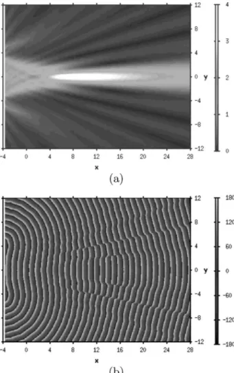
The issue is well illustrated in Fig.8, which shows both the 2D power and phase patterns behind the lens. The phase pattern in Fig.8(b)shows the phase slippage that occurs in the focal area in the process of wave focusing. The actual phase slippage in this example happens at

xP⬇14␭, i.e., about halfway between the maximum power

focal point and the geometrical focus.

4. CONCLUSIONS

We proposed and analyzed a few asymptotic wavelike ap-proximations for the accurate and efficient modeling of di-electric lenses used in quasi-optical systems of millimeter, submillimeter, and infrared wave applications. For com-parison, we developed an exact full-wave analytic solution of a two-dimensional focusing lens problem and used it as a benchmark for testing and validation of the asymptotic models being proposed.

The main asymptotic formulations considered are the two-term Kirchhoff model with an appropriate approxi-mation of the normal derivative of complex wave ampli-tude at the lens surface (KU) and the one-term Rayleigh– Sommerfeld diffraction integral formulation modified for nonplanar (curved) exit lens surfaces (RS2). The Rayleigh–Sommerfeld approximation modified for curved surfaces (RS2 model) is found to be more general and bet-ter suited for various kinds of dielectric lenses including symmetric and asymmetric, thin and thick, and rather large and relatively small lenses.

Both the Kirchhoff model (KU) and the Rayleigh– Sommerfeld representation modified for nonplanar sur-faces (RS2) are remarkably accurate for large lenses 共f,DⰇ␭兲, where no total internal reflection effects occur (i.e., typically for symmetric lenses or sufficiently thin asymmetric ones with a relatively flat exit surface).

Both the KU and RS2 approximations are also surpris-ingly accurate for small lenses, including the microlenses, when both the lens diameter D and the focal length f are comparable with the radiation wavelength ␭共f⬃D⬃␭兲, though small lenses have to be symmetric for minimizing the possibility of total internal reflection effects. The KU model fails, however, for bulk asymmetric lenses with a rather convex exit surface, where the total internal reflec-tion occurs for the waves near the lens rim.

ACKNOWLEDGMENT

The authors are grateful to J. A. Murphy for useful dis-cussions.

REFERENCES

1. C. O’Sullivan, G. Cahill, J. A. Murphy, W. K. Gear, J. Harris, P. A. R. Ade, S. E. Church, K. L. Thompson, C. Fig. 8. (a) Power and (b) phase patterns computed by an exact

Pryke, J. Bock, M. Bowden, M. L. Brown, J. E. Carlstrom, P. G. Castro, T. Culverhouse, R. B. Friedman, K. M. Ganga, V. Haynes, J. R. Hinderks, J. Kovak, A. E. Lange, E. M. Leitch, O. E. Mallie, S. J. Melhuish, A. Orlando, L. Piccirillo, G. Pisano, N. Rajguru, B. A. Rusholme, R. Schwarz, A. N. Taylor, E. Y. S. Wu, and M. Zemcov, “The quasi-optical design of the QUaD telescope,” Infrared Phys. Technol. 51, 277–286 (2008).

2. A. Walther, The Ray and Wave Theory of Lenses

(Cambridge U. Press, 2006).

3. C. A. Balanis, Advanced Engineering Electromagnetics (Wiley, 1989).

4. P. Wenig, M. Schneider, and R. Weigel, “Performance analysis of a cylindric dielectric lens antenna for 77 GHz Automotive Radar,” in Proceedings of International Radar

Symposium (IRS 2008), 21–23 May 2008, Wroclaw, Poland,

A. Kawalec and P. Kaniewski, eds. (Institute of Radioelectronics, 2008), paper B1-1.

5. D. Feng, Y. Yan, G. Jin, and S. Fan, “Axial focusing characteristics of diffractive microlenses based on a rigorous electromagnetic theory,” J. Opt. A, Pure Appl. Opt.

6, 1067–1071 (2004).

6. J.-S. Ye, B.-Z. Dong, B.-Y. Gu, G.-Z. Yang, and S.-T. Liu, “Analysis of a closed-boundary axilens with long focal depth and high transverse resolution based on rigorous electromagnetic theory,” J. Opt. Soc. Am. A 19, 2030–2035 (2002).

7. J.-S. Ye, B.-Y. Gu, B.-Z. Dong, and S.-T. Liu, “Application of improved first Rayleigh–Sommerfeld method to analyze the performance of cylindrical microlenses with different

f-numbers,” J. Opt. Soc. Am. A 22, 862–869 (2005).

8. K. Duan and B. Lu, “Improved diffraction integral for studying the diffracted field of a spherical microlens,” J. Opt. Soc. Am. A 22, 2677–2681 (2005).

9. M. N. O. Sadiku, Numerical Techniques in Electromagnetics (CRC, 1992).

10. C. Muller, Foundations of the Mathematical Theory of

Electromagnetic Waves (Springer-Verlag, 1969).

11. D. W. Prather, M. S. Mirotznik, and J. N. Mait, “Boundary integral methods applied to the analysis of diffractive optical elements,” J. Opt. Soc. Am. A 14, 34–43 (1997). 12. G. Fikioris, “A note on the method of analytical

regularization,” IEEE Antennas Propag. Mag. 43, 34–40 (2001).

13. S. V. Boriskina, P. Sewell, T. M. Benson, and A. I. Nosich, “Accurate simulation of two-dimensional optical microcavities with uniquely solvable boundary integral equations and trigonometric Galerkin discretization,” J. Opt. Soc. Am. A 21, 393–402 (2004).

14. A. V. Boriskin, A. I. Nosich, S. V. Boriskina, T. M. Benson, P. Sewell, and A. Altintas, “Lens or resonator? Electromagnetic behavior of an extended hemielliptic lens for a submillimeter-wave receiver,” Microwave Opt. Technol. Lett. 43, 515–518 (2004).

15. V. B. Yurchenko and A. Altintas, “Asymptotic wave-like modeling of dielectric lenses,” in Proceedings of the 6th

International Conference on Antenna Theory and Techniques (ICATT 2007), 17–21 September 2007, Sevastopol, Ukraine, Y. S. Shifrin and N. N. Kolchigin, eds. (IEEE, 2007), pp. 93–98.

16. Y. Li and E. Wolf, “Focal shifts in diffracted converging spherical waves,” Opt. Commun. 39, 211–215 (1981).