High-efficiency arrays of inductive coils

(1)

HIGH-EFFICIENCY ARRAYS OF

INDUCTIVE COILS

a thesis

submitted to the department of electrical and

electronics engineering

and the graduate school of engineering and science

of bilkent university

in partial fulfillment of the requirements

for the degree of

master of science

By

Erdal G¨

onendik

July, 2014

(2)

I certify that I have read this thesis and that in my opinion it is fully adequate, in scope and in quality, as a thesis for the degree of Master of Science.

Assoc. Prof. Dr. Hilmi Volkan Demir (Advisor)

Prof. Dr. Ayhan Altınta¸s

Assist. Prof. Dr. Yi˘git Karpat

Approved for the Graduate School of Engineering and Science:

Prof. Dr. Levent Onural Director of the Graduate School

(3)

ABSTRACT

HIGH-EFFICIENCY ARRAYS OF INDUCTIVE COILS

Erdal G¨onendik

M.S. in Electrical and Electronics Engineering Supervisor: Assoc. Prof. Dr. Hilmi Volkan Demir

July, 2014

Inductive heating is widely exploited in industrial operations including metal hardening, forging and brazing. Recently, as a promising alternative to tradi-tional heating, inductive heating has attracted substantial commercial interest for domestic cookers. This is because inductive heating offers fast, precise and efficient heating compared to traditional methods that make use of either con-vection or conduction as a means of heat transfer. To introduce full flexibility in using the cooking space, a strong demand is currently directed toward all-surface induction ovens, with the capability to heat a vessel placed arbitrarily anywhere on the surface of the induction cook top. For this purpose, inductive coils of tens of mm in diameter are required to be designed and stacked together to form coil arrays. However, this typically comes at the cost of reduced efficiency. To address this problem, this thesis work focuses on high-efficiency coil arrays designed for all-surface induction with optimum ferrite placement. Here analytical, numerical and experimental electromagnetic analyses of sample coils are performed. Ef-fects of different ferrite placements are investigated and, contrary to the general intuition of placing ferrite bars only under the coil, an effective way of ferrite placement is proposed and shown. These results indicate that the proposed high-efficiency arrays of inductive coils are highly promising for all-surface inductive heating.

(4)

¨

OZET

Y ¨

UKSEK VER˙IML˙I ˙IND ¨

UKT˙IF BOB˙IN D˙IZ˙INLER˙I

Erdal G¨onendik

Elektrik ve Elektronik Mühendisli˘gi, Yüksek Lisans Tez Yöneticisi: Do¸c. Dr. Hilmi Volkan Demir

Temmuz, 2014

˙Indüktif ısıtma endüstride metal döküm, prin¸c ile lehimleme ve demir dövmecili˘ginde yaygın olarak kullanılmaktadır. Yakın ge¸cmi¸ste indüktif ısıtmanın ev ocaklarında kullanılmasının gelenekesel ocaklara gü¸clü bir alternatif te¸skil etmesi, indüktif ocaklara kar¸sı büyük bir ticari ilgi uyandırdı. Bunun nedeni indüktif ısıtmanın normal ocaklarda kullanılan konveksiyon (do˘galgazli ocak-lar) veya temas (elektrik rezistanslı ocakocak-lar) yolu ile ısıtma metodlarına göre hızlı, hassas ve verimli olmasıdır. Günümüzde, gözlü indüktif ocaklarda ocak yüzeyinin tamamının esnek olarak kullanılabilmesini, di˘ger bir deyi¸sle ısıtılacak tencerenin ocak yüzeyinin herhangi bir yerine konularak ısıtılmasını mümkün kılmak i¸cin tüm yüzey indüktif ocak olarak anılan yapılara do˘gru gü¸clü bir yönelim olu¸smu¸stur. Bu ama¸c do˘grultusunda ¸capları onlarca mm olan kü¸cük bobinlerin tasarlanması ve bu bobinler ile uygun dizinler olu¸sturulması gerekmek-tedir. Fakat bu bobinlerin yanyana konulmaları ocak verimini dü¸süren bir etki yaratmaktadır. Bu problemi ¸cözmek i¸cin bu tezde yüksek verimli bobin dizinleri ve bu dizinler i¸cin optimal ferrit yerle¸simi üzerine yo˘gunla¸sılmı¸stır. Burada bazı ¨

ornek bobinlerin analitik, sayısal ve deneysel elektromanyetik ¸calı¸smaları yapılıp, farklı ferrit yerle¸simleri incelenmi¸stir. Genel bir kanı olan ferrit ¸cubukların sadece bobinlerin altına yerle¸stirilmesinin aksine farklı ve optimal bir ferrite yerle¸simi ¨

onerilmi¸stir. Elde edilen sonu¸clar önerilen yüksek verimli bobin dizininin tüm yüzey indüktif ocaklar i¸cin umut verici oldu˘gunu göstermektedir.

Anahtar sözcükler : RF bobinler, bobin dizinleri, indüktif ısınma, tüm yüzey indüktif ocaklar.

(5)

Acknowledgement

I would like to express my special appreciation and thanks to my advisor Professor Dr. Hilmi Volkan Demir, you have been a tremendous mentor for me. I would like to thank you for encouraging my research work and for allowing me to grow as a research scientist. Your advice on both research as well as on my career have been priceless. I would also like to thank my committee members, Professor Ayhan Altınta¸s and Professor Yi˘git Karpat for serving as my committee members. Many thanks to you. I would especially like to thank my colleagues Emre ¨Unal and Veli T. Kılı¸c for helping me out to build the experimental setup and fabricate the prototypes. I would like to thank Namık Yılmaz, lead design engineer at Ar¸celik power electronics department and all other Ar¸celik R&D engineers and managers for their helpful advices and discussions. Also thanks to M˙IKES Inc. for giving me the opportunity to study towards M.Sc.

A special thanks to my family. Words cannot express how grateful I am to my mother, father siblings for all of the sacrifices that you have made on my behalf. Your prayer for me was what kept me going thus far. I would also like to thank all of my friends who supported me in writing. This thesis work is supported by SANTEZ, for which I am very grateful and happy to acknowledge.

(6)

List of Figures

2.1 A simple induction heating system with coil (yellow), load to be heated (cyan) and ferrite substrate (red). . . 5 2.2 A filamentary turn between two finite thickness substrate of certain

material properties. . . 6 2.3 Magnitude of the magnetic field in z direction at different distances

from the coil. The coil is unloaded and no ferrite is used. . . 12 2.4 Magnitude of the magnetic field in the r-direction for different

dis-tances from the coil. . . 13 2.5 Magnitude of electric field in the φ-direction. . . 14 2.6 Magnitude of Bz at different distances from the coil when the coil

is driven at 100 kHz. . . 15 2.7 Magnitude of Bz when the ferrite is placed under the coil. . . 16

2.8 Magnitude of Bz for three different loads (a) without ferrite and

(b) with ferrite. . . 17 2.9 Magnitude of Eφ for three different loads (a) without ferrite, (b)

with ferrite. . . 17

(9)

LIST OF FIGURES ix

3.2 Measurement technique I. . . 20 3.3 Measurement technique II. . . 21 3.4 Voltage induced in the pickup coil in V (left y axis) and hall probe

reading in gauss (right axis). . . 21 3.5 Front picture of Coil 1. . . 23 3.6 Measurement results of Bz at different distances from unloaded

Coil 1 (a) without ferrite and (b) with ferrite. . . 23 3.7 Simulation results of Bz at different distances from unloaded Coil

1 (a) without ferrite and (b) with ferrite. . . 24 3.8 All surface scan of Bz at 5 mm above unloaded Coil 1 (a) without

ferrite and (b) with ferrite. . . 25 3.9 Measurement results of Bzat different distances from Coil 1 loaded

with the ferromagnetic steel (a) without ferrite and (b) with ferrite. 27 3.10 Simulation results of Bz at different distances from Coil 1 loaded

with the ferromagnetic steel (a) without ferrite and (b) with ferrite. 27 3.11 Measurement results of Bzat different distances from Coil 1 loaded

with aluminum (a) without ferrite and (b) with ferrite. . . 28 3.12 Simulation results of Bz at different distances from Coil 1 loaded

with aluminum (a) without ferrite and (b) with ferrite. . . 28 3.13 Measurement results of Bz at different distances from unloaded

Coil 2 (a) without ferrite and (b) with ferrite. . . 30 3.14 Simulation results of Bz at different distances from unloaded Coil

2 (a) without ferrite and (b) with ferrite. . . 31 3.15 All surface scan of Bz at 5 mm above unloaded Coil 2 (a) without

(10)

LIST OF FIGURES x

3.16 Measurement results of Bzat different distances from Coil 2 loaded

with ferromagnetic steel (a) without ferrite and (b) with ferrite. . 32 3.17 Measurement results of Bzat different distances from Coil 2 loaded

with aluminum (a) without ferrite and (b) with ferrite. . . 32 3.18 Pictures of Coil 3 (a) front view and (b) back view. . . 33 3.19 All-surface scan of Bz at 8 mm above unloaded Coil 3 (a) profile

view and (b) top view. . . 34 3.20 All surface scan of Bz at 8 mm above Coil 3 loaded with

ferromag-netic steel (a) profile view and (b) top view. . . 35 3.21 All surface scan of Bz at 8 mm above Coil 3 loaded with aluminum:

(a) profile view and (b) top view. . . 36 3.22 Analyzed Coil 4:(a) rear view, (b) front view and (c) side view. . . 37 3.23 All surface scan of Bz at 8 mm above unloaded Coil 4(a) profile

view and (b) top view. . . 38 3.24 Measurement results of Bzat different distances from Coil 4 loaded

with(a) ferromagnetic steel and (b)aluminum. . . 38 3.25 All surface scan of Bz at 8 mm above Coil 4 loaded with

ferromag-netic steel (a) profile view and (b) top view. . . 39 3.26 Prototype structure. . . 40 3.27 All surface scan of Bz at 5 mm above the prototype coil with an

inner radius of 19.0 mm and loaded with the ferromagnetic steel: (a) measurement and (b) simulation. . . 42 3.28 All surface scan of Bz at 5 mm above the prototype coil with an

inner radius of 30.5 mm and loaded with the ferromagnetic steel: (a) measurement and (b) simulation. . . 42

(11)

LIST OF FIGURES xi

3.29 All surface scan of Bz at 5 mm above the prototype coil with an

inner radius of 39.7 mm and loaded with the ferromagnetic steel: (a) measurement and (b) simulation. . . 43 3.30 Measurement of Bz at 5 mm above the prototype coil with different

inner radius values loaded with the ferromagnetic steel. . . 43 3.31 Change in the electrical loss in the load. . . 44 3.32 Change in efficiency as a function of the inner radius. . . 44 3.33 All surface scan of Bz at 5 mm above the prototype coil loaded

with the ferromagnetic steel when (a)the radius is 31 mm and (b) the radius is 41 mm. . . 46 3.34 All surface scan of Bz at 5 mm above the prototype coil loaded

with the ferromagnetic steel when (a)the radius is 51 mm and (b) the radius is 61 mm. . . 47 3.35 Change in the electrical loss in the load. . . 47 3.36 Change in efficiency as a function of the inner radius. . . 47

4.1 Gain in the electrical loss (a) for different ferrite µr and (b)for

different ferrite thicknesses. . . 49 4.2 Simulation results of magnetic field components in Region 1 with

ferrite (red plot) and without ferrite (blue plot): (a) Br and (b)Bz. 50

4.3 Simulation results of magnetic field components in Region 2 with ferrite (red plot) and without ferrite (blue plot): (a) Br and (b)Bz. 51

4.4 Simulation results of magnetic field components in Region 3 with ferrite (red plot) and without ferrite (blue plot): (a) Br and (b)Bz. 51

(12)

LIST OF FIGURES xii

4.6 Surface scan of Bz at 5 mm above Coil 1 loaded with the

fer-romagnetic steel, no ferrite bar is used: (a) simulation, (b) measurement top-view and (c) measurement perspective-view. . . 53 4.7 Surface scan of Bz at 5 mm above Coil 1 loaded with the

fer-romagnetic steel, 2 ferrite bars are used: (a) simulation, (b) measurement top-view and (c) measurement perspective-view. . . 54 4.8 Surface scan of Bz at 5 mm above Coil 1 loaded with the

ferro-magnetic steel, 10 ferrite bars are used: (a) simulation, (b) measurement top-view and (c) measurement perspective-view. . . 56 4.12 Change in the average induced voltage in pickup coil as a function

of the number of ferrite bars. . . 56 4.13 Simulation results of change in the electrical loss in the load with

increasing number of ferrite bars used with (a) aluminum load and (b)ferromagnetic steel load. . . 57 4.14 Generic illustration of the analyzed structures. . . 58 4.15 Surface scan of Bz at 5 mm above Coil 1 loaded with the aluminum

when the angle between the ferrite bars is 40°: (a) simulation, (b) measurement top-view and (c) measurement perspective-view. 59

(13)

LIST OF FIGURES xiii

4.16 Surface scan of Bz at 5 mm above Coil 1 loaded with the aluminum

when the angle between the ferrite bars is 50°: (a) simulation, (b) measurement top-view and (c) measurement perspective-view. 59 4.17 Surface scan of Bz at 5 mm above Coil 1 loaded with the aluminum

when the angle between the ferrite bars is 90°: (a) simulation, (b) measurement top-view and (c) measurement perspective-view. 61 4.21 Average voltage induced in the pickup coil at 5mm above Coil 1

loaded with the (a) aluminum and (b)ferromagnetic steel. . . 62 4.22 Electrical loss in the load changing with the angle between the

ferrite bars when Coil 1 is loaded with the (a) aluminum and (b)ferromagnetic steel. . . 63 4.23 Generic illustration of the analyzed structures. . . 63 4.24 Surface scan of Bz at 5 mm above Coil 1 loaded with the

ferro-magnetic steel when the angle between the longest side of the ferrite bar and coil radial axis is 0°:(a) simulation, (b) measurement top view and (c) measurement perspective view. . . 64

(14)

LIST OF FIGURES xiv

4.25 Surface scan of Bz at 5 mm above Coil 1 loaded with the

ferro-magnetic steel when the angle between the longest side of the ferrite bar and coil radial axis is 45°:(a) simulation, (b) measurement top view and (c) measurement perspective view. . . 64 4.26 Surface scan of Bz at 5 mm above Coil 1 loaded with the

ferro-magnetic steel when the angle between the longest side of the ferrite bar and coil radial axis is 90°:(a) simulation, (b) measurement top view and (c) measurement perspective view. . . 65 4.27 Average voltage induced in the pickup coil for different ferrite

placements. . . 66 4.28 Change in the electrical loss in the load with angle between the

longest side of ferrite bar and coil radial axis when the coil is loaded with the (a) aluminum and (b)ferromagnetic steel. . . 66 4.29 Generic illustration of the analyzed structures. . . 67 4.30 Surface scan of Bz at 5 mm above Coil 1 loaded with the

alu-minum, when the ferrite thickness is 5 mm: (a) simulation, (b) measurement top-view and (c) measurement perspective-view. . . 68 4.31 Surface scan of Bz at 5 mm above Coil 1 loaded with the

alu-minum, when the ferrite thickness is 10 mm: (a) simulation, (b) measurement top-view and (c) measurement perspective-view. 69 4.32 Surface scan of Bz at 5 mm above Coil 1 loaded with the

alu-minum, when the ferrite thickness is 15 mm: (a) simulation, (b) measurement top-view and (c) measurement perspective-view. 70 4.33 Experimentally measured average voltage induced in the pickup

coil using different ferrite thicknesses when the coil is loaded with the (a) aluminum and (b)ferromagnetic steel. . . 71

(15)

LIST OF FIGURES xv

4.34 Numerically simulated change in the electrical loss in the load as a function of ferrite thickness when the coil is loaded with the (a) aluminum and (b)ferromagnetic steel. . . 71 4.35 Generic illustration of the analyzed structures. . . 72 4.36 Surface scan of Bz at 5 mm above Coil 1 loaded with the

ferro-magnetic steel when all 8 ferrite bars are placed under the coil:(a) simulation, (b) measurement top-view and (c) measure-ment perspective-view. . . 73 4.37 Surface scan of Bzat 5 mm above Coil 1 loaded with the

ferromag-netic steel when 6 ferrite bars are placed under the coil and 2 are placed around the inner peripheral:(a) simulation, (b) measurement top-view and (c) measurement perspective-view. . . 74 4.38 Surface scan of Bz at 5 mm above Coil 1 loaded with the

ferro-magnetic steel when 4 ferrite bars are placed under the coil, 2 are placed around the inner peripheral and 2 are placed above the coil:(a) simulation, (b) measurement top-view and (c) measurement perspective-view. . . 74 4.39 Generic illustration of the analyzed structures. . . 75

5.1 Pictures of the elliptic coil:(a) front-view and (b) back-view. . . . 78 5.2 All surface scan of Bz at 5 mm above the single unloaded elliptic

coil:(a) measurement perspective-view and (b) measurement top-view. . . 79 5.3 All surface scan of Bz at 5 mm above the single elliptic coil loaded

with the ferromagnetic steel:(a) measurement perspective-view and (b) measurement top-view. . . 79

(16)

LIST OF FIGURES xvi

5.4 Simulation results for Bz at 5 mm above the single elliptic coil

loaded with the ferromagnetic steel:(a) surface scan of Bz and (b)

Bz traced on the minor axis. . . 80

5.5 Coil structure used for simulations:(a) perspective-view and (b) front-view. . . 81 5.6 Measured all surface scan of Bz at 5 mm above the two unloaded

elliptic coils driven at a phase difference of (a) 0°and (b) 180°. . . 82 5.7 Simulated all surface scan of Bz at 5 mm above the two unloaded

elliptic coils driven at a phase difference of (a)0°and (b) 180°. . . . 82 5.8 Measured all surface scan of Bz at 5 mm above the two elliptic

coils loaded with ferromagnetic steel(a) at 0°and (b) at 180°. . . . 83 5.9 Simulated all surface scan of Bzat 5 mm above the two elliptic coils

loaded with ferromagnetic steel and driven at a phase difference of (a) 0°and (b)180°. . . 83 5.10 Measured Bz at 5 mm above the single and double elliptic coils

when the coils are (a)unloaded and (b)loaded with the ferromag-netic steel. . . 84 5.11 (a) Illustration of the direction along which Bz is measured and

(b)Bz at 5 mm above the double elliptic coils along the blue line

(17)

List of Tables

4.1 Average voltage induced in the pickup coil. . . 75 4.2 Electrical loss in the load. . . 76

(18)

Chapter 1 Introduction

Induction heating technology has been used in industry in a wide variety of ap-plications including heat treating, welding and annealing cooking among many others [1, 2]. The idea of using induction heating in domestic appliances such as induction ovens goes back to 1973 [3]. In those days domestic induction hubs were becoming popular, due to its features of safety, fast heating, high efficiency, precise control of heat transfer, and cleanliness compared to other conventional heating techniques of convection and conduction heating. Most of these features are because of the fact that the heating in induction heating occurs right in the vessel due to the eddy currents and the joules heating generated in the vessel.

In domestic induction ovens the desired heating in the metallic vessel is gen-erated by a time-varying magnetic field. This time-varying magnetic field is generated by a planar coil powered by a power inverter. This planar turn is placed right below a metallic vessel. Domestic induction ovens typically consist of mainly three components: inductor and magnetic components, power inverter and digital controller.

The first component of an induction oven is the power converter part. Induc-tion ovens take the energy from the mains voltage. This voltage is rectified and bus filtered to allow a high voltage ripple to get an input power factor close to one. Then the power is delivered to the inductor-load couple by varying the frequency

(19)

of the voltage using resonant inverter topologies. Most common topologies em-ployed in induction ovens are full-bridge [4, 5], half-bridge [6–10] and two single switch inverter topologies: a ZVS one [11,12] and a ZCS one [13]. These days due to its robustness and cost savings most popular topology used is the half-bridge topology [14]. In today’s research end development, this half-bridge topology is still being studied and developed to for new application specific topologies. For example, in [15–17] topologies for heating two or more loads simultaneously are reported. In [18] half-bridge topology to feed three separate concentric windings simultaneously is presented. In [19], for large signal characterization of inductive loads, a series-resonant half-bridge inverter module that delivers up to 7kW power is reported. Power converters are not the main focus of this thesis, however it is essential for a successful coil design to understand how the coil is driven.

The second component, which is the main focus of this thesis, is the induction coil and magnetic materials used with it. Induction coils transfer the electrical power delivered by the power inverter to the load by means of magnetic coupling. To deliver the power to a flat vessel more effectively, flat-type spiral windings are commonly used [20, 21]. Here external diameter of a coil is defined by the size of the burners. In other words, the size of the coil is chosen to be as large as the load intended to be used for that burner. Then, number of turns is determined depending on the inductor value required by the power inverter and maximum power desired to be delivered to the load. For efficiency considerations, the num-ber of strands used in the coil is set to decrease the loss in the coil as much as possible [22]. Analysis of the equivalent impedance of the designed coil [23, 24] can be used as a feedback to the resonant inverter for further optimization of the system.

In today’s induction ovens as mentioned above, one coil is designed for each burner on the cook top. This allows the user to put the vessel only where the burner is at. To increase the flexibility in using the surface of the cook top, all-surface induction oven has become the hot topic of domestic induction heating. In all-surface ovens, inductive coils of tens of mm in diameter are required to be designed and stacked together to form coil arrays so the the user can put the vessel anywhere s/he likes on the cook top and the vessel is heated by powering

(20)

up the coils only under the vessel. However, due to coupling effect between the coils of small diameters, the power delivery efficiency of the system is greatly reduced and this is an important problem of current all-surface induction ovens to be addressed.

The main purpose of this thesis is to design high-efficiency coil arrays to be used in all-surface induction ovens with ferrite placement. For this purpose in Chapter 2 analytical model of a simple case where one planar coil is sandwiched between a load and ferrite is derived. Using this model, effect of the ferrite is investigated. Also effect of the material properties of the load placed at different distances to the coil on the heating is investigated. In Chapter 3, numerical electromagnetic analyses of some sample coils currently used in induction ovens of different types are performed using CST Electromagnetic Studio (CST EMS), followed by experimental analyses to confirm the obtained results. In Chapter 4, performance enhancement in utilization of ferrite is investigated in detail, and comparisons of different ferrite placement is performed. With the knowledge obtained from Chapters 2-4, finally in Chapter 5 we study coil array stacking. The studied array scheme has been shown to outperform common coil arrays used today. Three patent applications have been made as a result of this thesis work.

(21)

Chapter 2 Inductive Heating

In Figure 2.1, a simple induction heating system typically used in induction ovens is shown with a planar coil and load put above it. Here the red substrate is the ferrite used to enhance the magnetic field component in the z direction. In this setup the coil is fed with a sinusoidal current to generate a sinusoidal magnetic field in the system. This magnetic field creates a time-varying magnetic flux on the bottom of the load and this forms eddy currents that heat up the load. This heating is directly proportional to the square of the current driving the coil. In a typical induction oven, the current levels are commonly in the range of 20-100 A depending on the application. As the frequency of the current driving the coil is increased, the heat generated in the load is also increased. However, due to practical limitations, the frequency of operation is commonly set around tens of kHz and usually does not exceed 100 kHz. Increasing the frequency of operation causes some practical problems. As the frequency is increased, parasitic capaci-tances between windings of the coil become more sound and this deteriorates the operation. In addition to this, being able to switch currents of peak values of tens of amperes at higher frequencies requires more costly transistors. In order to deliver real power to the load most efficiently, the system must be working at the resonant frequency. Thus, another practical limitation on the frequency of operation is the availability of low value power capacitors that can be used in the power electronics of such a system. To make the operating frequency higher, the

(22)

capacitance of the corresponding capacitor that the electronics will require to be using to put the system in resonance will go lower. Given a rough estimate of the inductance of the system, the only factor that determines the capacitor value to be used for resonance is the operating frequency. Larger frequencies simply require smaller capacitor values. And power capacitors with lower capacitance values are harder to find in the market. With all these considerations, the ap-propriate operating frequency of an induction heating system is typically in the range of 20-100 kHz; for example, a common operating frequency is 30 kHz.

Figure 2.1: A simple induction heating system with coil (yellow), load to be heated (cyan) and ferrite substrate (red).

2.0.1 Analytical Background

Typical coil diameters in an induction oven changes in the range of 70 to 2000 mm. As discussed above, a common operating frequency is around 30 kHz. Therefore, the wavelength of the resulting fields is 10 km. Apparently, physical dimensions of the system compared to the wavelength of the fields generated in the sys-tem is very small. This validates the assumption of quasi-static solution of the Maxwell’s equations. The displacement current term can be safely ignored. This conceptually means that there are not any electromagnetic waves generated by this system that propagate into the free space. Instead, there are stationary and time-varying fields in the system. With this assumption the problem is reduced to a magneto quasi-static problem. Applying Coulomb gauge condition ( ~∇. ~A = 0 ), the following equations apply to this system.

~

∇ × ~H = ~Jφ (2.1)

~

∇ × ~E = −∂ ~B

(23)

~

∇ × ~A = ~B (2.3) where ~E is the electric field vector, ~H is the magnetic field strength vector, ~A is the vector potential, ~B is the magnetic field and ~Jφ is the volumetric current

density in a circular winding.

Electromagnetic problem of a typical system used in induction ovens can be represented as shown in Figure 2.2. This shows the most general case for a filamentary turn used in a coil. If we analytically calculate the fields as a result of a single filamentary turn in six regions shown in the above figure, we can use superposition to calculate the final field distribution in the system by vectorially summing up the fields generated by each filamentary turn. Although here by applying superposition, we assume that the system is linear. In magnetic materials, such as the ferrite or the load with magnetic properties, there can occur two types of nonlinearities. These are magnetic hysteresis and saturation. In domestic pots normally soft magnetic materials are used with very little residual magnetization and, as a result, magnetic hysteresis can be ignored. Secondly, in induction ovens there always occurs a flux reduction due to induced currents in load and usually the material works far off its saturation point. Also in this thesis work, during the experiments where we used aluminum as the load we did not feed the coil with very high current levels (below 20 A). As a result magnetic saturation can also safely be ignored.

Figure 2.2: A filamentary turn between two finite thickness substrate of certain material properties.

(24)

The procedure that will be followed here to analytically solve the electromag-netic problem depicted in Figure 2.2 is carried out in [25] for the infinite substrate. The method in [25] is the same method as we use here, which is based on the Fourier-Bessel integral transformation. In [26] and [27], inductive components of the filamentary formulas are derived using the method of images. An alternative method is used in [28] for infinite substrate utilizing magnetic vector potential. Another method that uses magnetic vector potential is [29]. In [29], each of the substrates is defined to possess a finite thickness and many layers of materials are defined both above and below the filamentary turn. Our approach to the problem is also given in [30]. Here we further elaborated on the results of [30] for different regions given in Figure 2.2 and implemented the closed form solutions of the fields in these regions using MATLAB.

We assume that the filamentary turn with radius a at z = d1 carries a

si-nusoidal current iφ = Iφejwt. The solution of the Maxwell’s equations must be

considered in six different regions as shown in Figure 2.2. Due to cylindrical symmetry of the problem we use cylindrical coordinates. Since the only external source in the system is in the φ-direction, we do not expect to see a magnetic field in the φ-direction, besides since the problem is considered to be magneto quasi-static and displacement current term in Maxwell’s equations is ignored, the only electric field we expect to see in the system is in the φ-direction. On the basis of cylindrical symmetry following identities hold for the electric field and the magnetic field.

Hφ = 0, ∂Hr ∂φ = 0, ∂Hz ∂φ = 0, Er = 0, Ez = 0, ∂Eφ ∂φ = 0 (2.4) After these observations, Maxwell’s equations reduce to the following equations in each region.

Region 1 (d1 ≤ z < d2): Utilizing the set of equalities given in Eq. (2.4)

and noticing that the only current source in the system is in the φ-direction, Eqs. (2.1) and (2.2) boil down to:

∂Hr ∂z − ∂Hz ∂r = Iφδ(r − a)δ(z − d1) ∂Eφ ∂z = jwµ0Hz

(25)

1 r

∂(rEφ)

∂r = −jwµ0Hz (2.5) Eliminating H gives the following equation for the only component of the electric field in the system.

∂2_E φ ∂z2 − ∂2_E φ ∂r2 + 1 r ∂Eφ ∂r − Eφ r2 = jwµ0Iφδ(r − a)δ(z − d1) (2.6)

Region 2 (0 ≤ z < d1): There is no current in this region, so equations

obtained for Region 1 can be simplified into the following equation for this region: ∂2_E φ ∂z2 − ∂2_E φ ∂r2 + 1 r ∂Eφ ∂r − Eφ r2 = 0 (2.7)

Region 3 (−m1 ≤ z < 0): In this region there is current due to the

conduc-tivity of this region (Jφ = σEφ), so the equation for Eφ in this region is reduced

to the following: ∂2Eφ ∂z2 − ∂2Eφ ∂r2 + 1 r ∂Eφ ∂r − ( 1 r2 + jwµ0µr3σ3)Eφ= 0 (2.8)

Region 4 (z < −m1): This region has no current thus, the simplified equation

for Eφ in this region is exactly the same as in Region 2.

Region 5 (d2 ≤ z < d2+ m): Equation for this region is identical to the one

we derived for Region 3, except that the material properties are different in this region. Therefore, the equation for Eφ in this region is given as follows:

∂2_E φ ∂z2 − ∂2_E φ ∂r2 + 1 r ∂Eφ ∂r − ( 1 r2 + jwµ0µr5σ5)Eφ= 0 (2.9)

Region 6 (d2+ m2 ≤ z): Equation for Eφin this region is similar to the ones

in Regions 2 and 4 and is given simply as in Eq. (2.7).

At this point, we are required to solve Eqs. (2.5) through (2.9). Once we solve these equations and obtain Eφ, we can find all the fields in each region.

To simplify equations given above, we use Fourier-Bessel integral transformation given as:

E_φ∗ = Z ∞

0

(26)

In Eq. (2.10), J1(kr) represents the Bessel function of the first kind of order

one. E_φ∗(k, z) is the transformed form of Eφ. For the sake of simplicity, we will

denote E_φ∗(k, z) simply as E∗. With this transform applied, Eq. (2.6) transforms into the following:

d2E∗ dz2 = k

2

E∗+ jwµ0IφaJ1(ka)δ(z − d1) (2.11)

The solution of this equation in Region 1 is in the form of :

E∗ = Aekz+ Be−kz (2.12) Note that this solution form also applies to Regions 2, 4 and 6.

In Regions 3 and 5 we have induced currents. So, applying Fourier-Bessel integral transformation to Eqs. (2.8) and (2.9), we obtain the following equations, respectively: d2E∗ dz2 = (k 2_{+ jwµ} 0µr3σ3)E ∗ (2.13) d2_E∗ dz2 = (k 2 + jwµ0µr5σ5)E ∗ (2.14) Solutions of the equations above are in the form of:

E∗ = Eeη3z_{+ F e}−η3z _(2.15)

E∗ = Keη5z_{+ Le}−η5z _(2.16)

where η5 = p(k2+ jwµ0µr5σ5) for Region 5 and η3 = p(k2+ jwµ0µr3σ3) for

Region 3.

Below is the summary of solutions for E∗ in each region:

Region 1 (d1 ≤ z < d2) :E∗ = Aekz+ Be−kz (2.17) Region 2 (0 ≤ z < d1) :E∗ = Cekz+ De−kz (2.18) Region 3 (−m1 ≤ z < 0) :E∗ = Eeη3z+ F e−η3z (2.19) Region 4 (z < −m1) :E∗ = Gekz+ He−kz (2.20) Region 5 (d2 ≤ z < d2 + m2) :E∗ = Keη5z+ Le−η5z (2.21) Region 6 (d2+ m2 ≤ z) :E∗ = Iekz+ M e−kz (2.22)

(27)

At first glance one can say that H = 0 and I = 0 since fields must vanish as z goes to negative and positive infinity. The electric field is also continuous at the boundaries of z = −m1, 0, d1, d2, d2+ m2. Equating E∗ at the boundaries result

in the following set of equations:

Ee−η3m1 _{+ F e}η3m1 _{= Ge}−km1 _(2.23)

C + D = E + F (2.24) Aekd1 _{+ Be}−kd1 _{= Ce}kd1 _{+ De}−kd1 _(2.25)

Aekd2 _{+ Be}−kd2 _{= Ke}η5d2 _{+ Le}−η5d2 _(2.26)

Keη5(d2+m2)_{+ Le}−η5(d2+m2)_{= M e}−k(d2+m2) _(2.27)

We have ten unknowns and five equations above. The other five equations come from the continuity of Hr. Hr is simply given by:

Hr=

1 jwµrµ0

∂E∗

∂z (2.28)

Since E∗ depends on z only, the exponent derivative of E∗ with respect to z can easily be taken. As a result, from the continuity of Hr at the boundaries where

there are no surface currents at z= −m1, 0, d2, d2+ m2 we arrive at the following

set of equations: k(C − D) = η3 µr3 (E − F ) (2.29) η3 µr3 (Ee−η3m1 _{− F e}η3m2_{) = kGe}−km1 _(2.30) k(Aekd2 _{− Be}−kd2_{) =} η5 µr5 (Keη5d2 _{− Le}−η5d2₎ _(2.31) η5 µr5 (Keη5(d2+m2)_{− Le}−η5(d2+m2)_{) = −kM e}−k(d2+m2) _(2.32)

One last equation comes from the boundary where we have the filamentary turn carrying the source current at z = d1. Hr can be easily found using E∗ from Eq.

(2.28). The boundary condition for Hr at the boundary z = d1 is given by:

~n × ( ~H1r − ~H2r) = δ(r − a)Iφ (2.33)

Here ~n is the vector normal to the plane of boundary. ~H1r and ~H2r are radial

(28)

have the Fourier-Bessel transforms of E∗ at hand in both Region 1 and 2. Using Eq. (2.28) we obtain the transform of ( ~H1r− ~H2r). To use Eq. (2.33), we need

to take the transform of δ(r − a)Iφ, which is indeed given as IφaJ1(ka). So, the

final boundary equation is found to be given as in Eq. (2.34). Aekd1 _{− Be}−kd1 _{− Ce}kd1 _{+ De}−kd1 ₌ jwµ0

k IφaJ1(ka) (2.34) Now we have ten unknowns of A, B, C, D, E, F, G, K, L, M and ten equations given by Eq. (2.23) to (2.27) and (2.29) to (2.34). The solution of this set of equations gives us E∗ in each of 6 regions. From here Hr can easily be obtained

using Eq. (2.28). The third field in the system, Bz, can also be easily calculated

using the equality:

Bz = 1 −jw[ E∗ r + ∂E∗ ∂r ] (2.35)

Finally for the transformed fields we need to take the inverse Fourier-Bessel Integral transform given by Eq. (2.36).

E = Z ∞

0

E∗(k)kJ1(kr)dk (2.36)

A MATLAB program was written to solve this set of equations. This pro-gram can compute any field in any region given the parameters including driving current level, frequency of operation, coil size, number of turns, diameter of each turn, turn separation, µr5, σ5, µr3, σ3, thicknesses of both load and ferrite, and

distance of the coil from load and/or ferrite. Also impedance of the system can be calculated so that inductance and resistance of the system are analyzed under different circumstances. This analytical solution helps us a lot to understand the behavior of the system. We can see how the system reacts to different types of loads and ferrite and how load and ferrite thicknesses affect the system. We can understand dependence of fields on the number of turns and coil sizes and also we have an idea of the inductance and resistance change of the system under differ-ent conditions. Below some simulation results are discussed. The effect of ferrite will further be more extensively discussed in Chapter 4. the following MATLAB runs were performed for a coil of 24 turns with a wire diameter of 1.3 mm. The inner radius of the coil is 25 mm and the outer radius of the coil is 88 mm. The

(29)

coil was driven with 30 A sinusoidal current. Figure 2.3 shows Bz at different

distances from the coil when the coil was driven at 50 kHz without any load or ferrite .

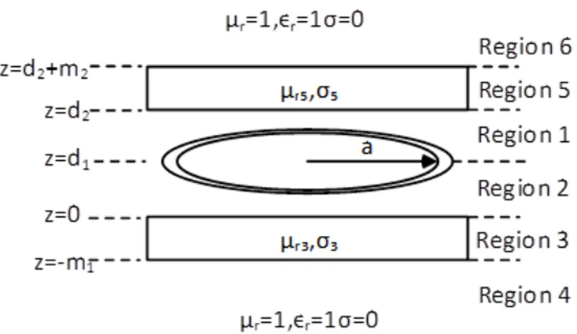
Figure 2.3: Magnitude of the magnetic field in z direction at different distances from the coil. The coil is unloaded and no ferrite is used.

It is apparent from Figure 2.3 that, as the distance from the coil increases, the magnetic field in the z-direction gets smaller in magnitude. Bz is the only

component of the fields in the system that creates a changing magnetic flux on the bottom of the vessel i.e., this is what heats up the load by induction and joule heating. This means that if the electronics of the system is capable of providing the coil with a constant current regardless of the impedance of the system, then the load should be put as close to the coil as possible. Couple of other important points that can be observed from Figure 2.3 is that the magnetic field peaks are located where the first turn starts at a distance of approximately 25 mm from the center of the coil in this case. The field then gradually decreases as we further move through other turns. At the 20th turn, the magnetic field sums up to zero and further down the way it starts to peak with a phase difference of 180◦, i.e., the magnetic field after the 20th _{turn is pointing down in the −z-direction whereas}

the magnetic field up to the 20th _{turn points in the +z-direction.}

(30)

Figure 2.4: Magnitude of the magnetic field in the r-direction for different dis-tances from the coil.

This component of the magnetic field does not contribute to the heating of the load since it does not create any changing flux in the load. Although the load has some finite thickness, its heating caused by Br due to this finite thickness is

negligible because this thickness is usually on the order of a couple of mm’s. Here also Br decreases as we move further away from the coil. Br stays quite constant

throughout the coil turns. Once the coil ends at around r = 88 mm Br decays

away very fast. This means, induction ovens would not cause any harm to the surrounding in the r-direction. In the z-direction, since there will always be a load while the system is running, due to the skin effect no field would be present above the load.

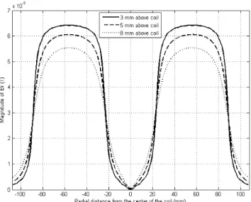
Figure 2.5 shows the electric field in the φ-direction. As expected Eφdecreases

as the distance from the coil is increased. This field peaks at the 14th _{turn and}

gradually decreases from there. Heating of the bottom of the load can also be thought to be caused by this Eφ. Actually this is what causes eddy currents in

the load. Looking at Figure 2.5 Eφ at d = 3 mm is quite larger than Eφ at d = 8

mm. This means that the load placed at d = 3 mm would be heated more than the load at d = 8 mm. The eddy current where Eφ peaks at about 60 mm away

(31)

pattern of the coil will be in circles and heating will first start around the circle with radius of 60 mm for this specific case.

Figure 2.5: Magnitude of electric field in the φ-direction.

Figure 2.6 shows the magnitude of Bz when the coil is driven at 100 kHz. As it

is obvious from this figure the fields do not depend on the frequency of operation when the coil is not loaded. Results in Figure 2.6 are exactly the same as results of Figure 2.3. However, as it will be analyzed later, when the coil is loaded, the frequency of operation matters. Increasing frequency will increase the loss in the load as it would increase the magnetic flux change on the bottom of the load.

Figure 2.7 shows Bz when a ferrite of 2 mm in thickness and µr = 500 is

placed 5 mm under the coil. In this case the coil is still not loaded with a vessel load and the operating frequency is at 50 kHz. When we compare Figure 2.3 with Figure 2.7 we observe the dramatic increase in the magnitude of Bz. We

can conclude that adding ferrite under the coil would increase the efficiency of the system because with the same amount of current one would expect more heating in the load or with less current one would reach the same level of heating compared to the case without ferrite. Effects of ferrite in induction heating will be analyzed in detail in Chapter 4 and, as a result of this analysis, optimum placement of ferrite will be determined.

(32)

Figure 2.6: Magnitude of Bz at different distances from the coil when the coil is

driven at 100 kHz.

materials of load is shown. All loads are taken to be 2 mm in thickness and are placed 3 mm above the coil and the rest of the parameters used in the simulation are the same as the previous ones. Here simulations were carried out with and without ferrite and effect of the ferrite is obvious in the plots. The three types of loads used in the simulations are made of aluminum with σ = 3.538 × 107Ω−1m−1 and µr = 1, copper with σ = 5.96 × 107Ω−1m−1 and µr = 1 and ferromagnetic

steel σ = 1.67 × 106_Ω−1_m−1 _{and µ}

r = 200. Since using ferromagnetic steel acts

like a ferrite with electrical loss, it further enhances the magnetic field between the coil and the load substantially compared to the aluminum and copper loads.

Figure 2.9 shows the electric field in the φ-direction when the coil is loaded with the three loads mentioned above. This figure tells us that the electrical loss (ohmic heating) in the ferromagnetic steel would be the highest. A very close look at Figure 2.9 reveals that the electrical loss in aluminum would be slightly larger than that in copper. This is because copper has a larger conductivity than the aluminum. Thus, aluminum has a larger resistance which results in a slightly larger electrical loss.

(33)

Figure 2.7: Magnitude of Bz when the ferrite is placed under the coil.

observe that Eφ is high in the r-direction only where coil turns exist and decays

sharply when turns end. This means that the heating in the load would be just like an image of the coil under it, i.e., the eddy currents flowing in the load takes the shape of the coil turns. This tells us, that if we would like to have a homogeneous heating in the load, the inner radius of the coil should approach to zero and the outer radius of the coil should exactly match the size of the load to be heated.

Finally, when we compare Bz at d = 3 mm in Figure 2.3 with Bz in Figure

2.8a for ferromagnetic steel, we see that the peak value of Bz drops by 18%.

This is due to the opposing magnetic field in the -z-direction created by the eddy currents generated in the load. Loading the coil also increases the amplitude of the valley depth from 32.59 to 36.32 G.

In this part, to understand the operation of an induction heating system we have analytically solved Maxwell’s equations and obtained expressions for each field of interest in the system. We have discussed how the fields change over distance across and away from the coil and with the frequency. Also we briefly mentioned the effect of using ferrite on the fields. Loading the coil with different types of materials change the efficiency of the system. Since ferromagnetic ma-terials act like a ferrite with strong electrical loss on them, they form a magnetic

(34)

(a) (b)

Figure 2.8: Magnitude of Bz for three different loads (a) without ferrite and (b)

with ferrite.

(a) (b)

Figure 2.9: Magnitude of Eφfor three different loads (a) without ferrite, (b) with

ferrite.

cavity for the coil and enhance magnetic fields in the system drastically, which in turn increases the efficiency of the system. Loads without magnetic properties like aluminum or copper do not form a magnetic cavity like ferromagnetic steel does; thus, it is harder to heat these materials compared to ferromagnetic steel. To heat these materials more current has to be driven into the system, which decreases the efficiency of the overall system.

(35)

Chapter 3 Electromagnetic Analyses of

Coils for Inductive Heating

3.1 Numerical

and

Experimental

Magnetic

Analysis of Coils

Analytical study presented in Chapter 2 gives us an insight about how the in-duction oven system works; however it has some shortcomings. First of all we model the wires as filamentary. Therefore the MATLAB simulations implement-ing the analytical model do not take the wire thickness into account. Secondly, the structure shown in Figure 2.2 represents a very general situation. Most of the time, coils with ferrite and load have more complex shapes and it is very hard to model such systems analytically even if it might be possible. To overcome these shortcomings we took a numerical approach using CST Electromagnetic Studio (CST EMS) to perform our simulations. In the rest of this thesis, unless oth-erwise stated, all numerical simulation results are obtained using CST EMS. To confirm these simulation results, we also built an experimental setup to measure the magnetic fields of different coils under loaded and unloaded conditions.

(36)

be described with the methodologies developed and used both in simulations and measurements. We also performed magnetic analyses of five different types of coils currently used in induction ovens. In the next part, both numerical simulations and experimental measurements of these coils will be discussed.

3.1.1 Experimental Setup and Measurement

Methodol-ogy

To measure the magnetic field in the z-direction we constructed a measurement setup as shown in Figure 3.1. This setup consists of a single turn pickup coil of 1 cm in diameter that is used to measure the magnetic field in the z-direction,along with a function generator, a power amplifier, an oscilloscope to measure the

volt-Figure 3.1: Measurement setup.

age induced in the pickup coil, a pc to process the data taken by the oscilloscope and to control xyz stage that allows us to move the pickup coil in 3D with a sensitivity of 50 µm.

In this setup, the function generator provides the power amplifier with a sin-gle tone signal at the desired amplitude and frequency. This signal is amplified in the power amplifier and fed to the coil. This creates a time-varying magnetic field in the system and this magnetic field induces a voltage in the pickup coil. This voltage value is read by the oscilloscope and transferred to the computer

(37)

using a MATLAB code. With the help of this code, xyz stage movement can also be controlled very precisely. During the measurement, the xyz stage moves con-tinuously on a predefined path while taking continuous measurements of induced voltage in the pickup coil. This way we obtain the magnetic field distribution (magnetic field map) of the system. With this setup we could load the coil with a load at any distance from the coil and still measure the magnetic field distribution between the coil and the load.

The voltage induced in the pickup coil is directly proportional to the frequency of operation, magnetic field amplitude at that location and the area of the pickup coil. Therefore, this voltage value gives us a very good idea about the magnetic field in the z-direction around pickup coil location. By changing the direction that the pickup coil looks, we could also measure the magnetic field in the r-direction in principle. However, here what we focus on is Bz because this component is

what heats up the load. The frequency of operation for the coil is very far away from the resonant frequency of the pickup coil, which is in MHz range. Thus, the measurements we took here are not distorted by the resonance of the pickup coil. With this setup we have take two different types of measurements. One is

Figure 3.2: Measurement technique I.

based on taking the measurement along a line above the coil at a certain distance from it as shown in Figure 3.2. The line along which we took the measurements goes through the center of the coil. The second measurement method is based on tracing the whole surface scan. As shown in Figure 3.3, the magnetic field on a plane parallel to the plane of coil and at any distance desired above it was measured and the result of this measurement is obtained as a surface plot.

(38)

Figure 3.3: Measurement technique II.

proportional to Bz at the pickup coil location. To validate this assumption we

compared the magnetic field that we measured using a Hall probe with the voltage induced in the pickup coil. For this measurement we used standard 24-turn coil coil 1 with a diameter of 180 mm (a product of Arelik). We derived the coil with a sinusoidal signal at 50 kHz. The coil was unloaded and no ferrite was used during this test. We measured the magnetic field 1 mm above the coil using the first measurement technique. While taking this measurement we also placed the Hall probe to make sure that it only reads magnetic field in the z-direction. The results are shown in Figure 3.4. In this figure the left y-axis is in volts and shows

Figure 3.4: Voltage induced in the pickup coil in V (left y axis) and hall probe reading in gauss (right axis).

(39)

G (10−4 T). It is obvious that these two measurements are consistent and this validates our measurement method. However, if it is desired to measure the exact absolute value of the magnetic field at a point very precisely, new methods need to be adapted. In this thesis, we are interested in the dependence of magnetic field in the z-direction on various parameters rather than its absolute value. Therefore, these measurement methods fulfill our requirements. Both of the measurement techniques above can be used for both loaded and unloaded coils. Using these two techniques of measurements, we analyzed different types of coils used in induction ovens and the results are discussed in detail in the next section.

At every analysis the impedance of the system is measured using an LCR meter. LCR meters measure the impedance of the system with small signal excitations. These measurements give quite a good idea about the behavior of the system however in practice what is usually required is the impedance of the system when the coil is fed with tens of amperes current.In [31] a test bench is designed to characterize the coils used for induction under high signal excitations and differences between LCR measurements and high signal excitation result are observed due to nonlinearity of the system under high signal condition. In this thesis LCR measurements are sufficient to make our point.

3.1.2 Case study: Coil 1 (circular cross-section coil)

In this part, the magnetic analysis of a 24-turn 180 mm-diameter coil (Coil 1) shown in Figure 3.5 is performed. This coil is utilized in some of the induction ovens (used by Arelik). This coil has an inner diameter of 45 mm. The cop-per wires used for the windings have circular cross sections and have a thickness of about 2.5 mm. As we mentioned before, what we care about in these mea-surements and simulations is the magnetic field in the z-direction. Due to the symmetry of the system in the φ-direction, we will mostly use the measurement technique I. Measurement technique II is also used from time to time to see the whole magnetic field map of the coil.

(40)

Figure 3.5: Front picture of Coil 1.

3.1.2.1 Unloaded Measurements and Simulations of Coil 1

In this part we performed simulations and measurements to analyze Bz of the

coil without any load above it. In both measurements and simulations, the coil is fed at 100 kHz with a 100 Vrms sinusoidal voltage source. The measurements and

simulations were carried out at three different distances from the coil. Figure 3.6

(a) (b)

Figure 3.6: Measurement results of Bz at different distances from unloaded Coil

1 (a) without ferrite and (b) with ferrite.

shows the magnetic field in the z-direction with and without ferrite. In measure-ments, we used ferrite bars of dimensions (5 mm × 15 mm × 60 mm) and we placed 8 of these bars under the coil. All ferrite bars were positioned aligning the longest dimension with the diameter of the coil, all pointing towards the center

(41)

of the coil and with the shortest dimension being perpendicular to the plane of the coil.

The measurement results are quite consistent with the results of the MAT-LAB simulations. As we further move away from the coil, the magnitude of Bz

decreases as expected. Here Bz with the ferrite is about 22% larger than the

case without the ferrite. The possible improvement with the ferrite is actually more than this, as we will examine in detail in Chapter 4. The reason why we obtain only a 22% improvement is due to how we feed the coil. We could drive the coil only with a constant voltage in this case. Putting ferrite under the coil increases its inductance. Without the ferrite, inductance of the coil is measured to be 59.12 µH. With ferrite bars, the inductance went up to 80 µH. The re-sistance of the system is due to only the rere-sistance of the coil which is around 88 mΩ. Thus, this resistance can simply be ignored in impedance calculation. Adding ferrite increased the impedance of the system by 35%, which means coil with ferrite drew 35% less current from the source since the voltage is constant. Smaller current results in smaller Bz and this limits the improvement of ferrite

to only 22%. If the coil was driven with a constant current source in both cases, the improvement in Bz due to the utilization of ferrite would be around 29%.

(a) (b)

Figure 3.7: Simulation results of Bz at different distances from unloaded Coil 1

(a) without ferrite and (b) with ferrite.

Figure 3.7 shows the CST EMS simulation results of the measurements above. The numerical results are quite consistent with the measurements. Ferrite bars

(42)

in the simulation were modeled with a µr value of 300. The gain in Bz in this

case is only 12.5%. This discrepancy in the improvement is due to the real value of µr of the ferrite. It is most probably above 500.

Magnetic field makes a dip towards the center of the coil where there are no turns as it is obvious from the plots above. The depth of this dip gets smaller as we move away from the coil in the z-direction. As seen in Figure 3.7, Bz gets

smoother around the center of the coil as the distance from the coil is increased from 5 to 13 mm. As the distance between the load and the coil is increased the effect of eddy currents to decrease the Bz in between load and coil is also

de-creased which results in higher inductance. This inductance change with respect to distance of the load to the coil is utilized in [32] to increase the efficiency of the power converter of the induction system.

One difference between the measurement and simulation results is that in simulations Bz towards the center of the coil makes a sharper dip than Bz in the

measurements. This is because of the averaging that the pickup coil does due to its finite size during the measurement. Since the pickup coil has a finite area, it sees all the magnetic flux coupled to its area. Therefore, instead of measuring Bz at a single point in space, it measures the sum of Bz at all points inside its

surface area. Being aware of this fact, this measurement technique still gives us an idea about the form of Bz.

(a) (b)

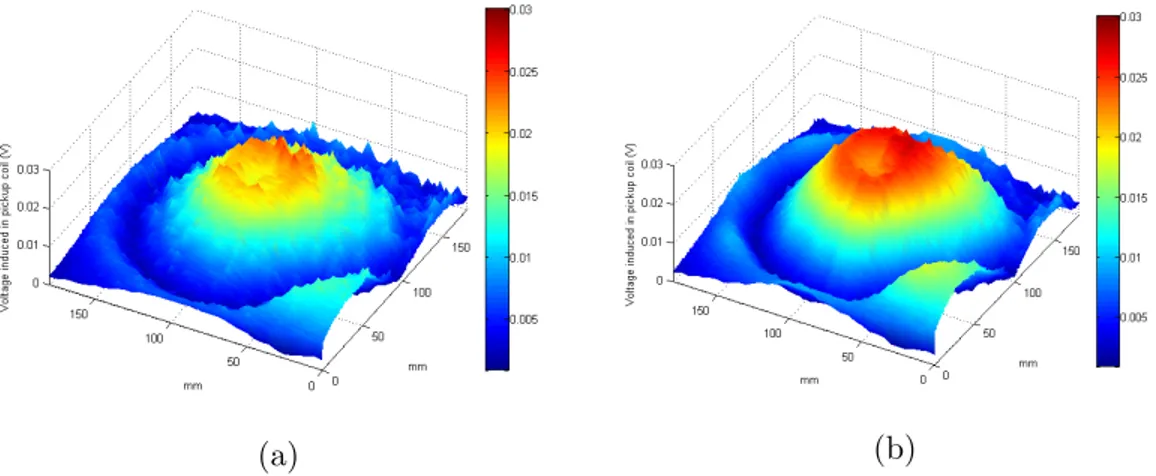
Figure 3.8: All surface scan of Bz at 5 mm above unloaded Coil 1 (a) without

(43)

Figure 3.8 shows the all-surface scan of Bz performed using measurement

technique II in Figure 3.3. Here the measurement was taken 5 mm above the coil. The symmetry of Bz in the φ-direction is obvious in these plots. The

magnetic field around the intersection of the x and y-axes is quite large in both Figure 3.8a and 3.8b. That is where the cable goes into the coil to make the first turn.

As a result, as we move away from the center of the coil in the +z-direction, the magnitude of Bz decreases and becomes smoother especially in the center of

the coil. We like to put the load as close to the coil as possible to heat it more efficiently.

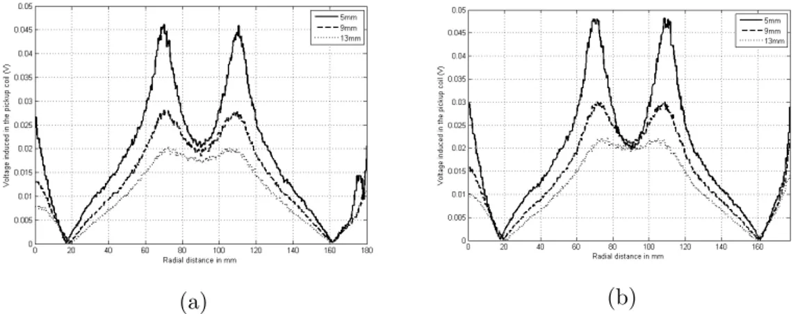
3.1.2.2 Loaded Measurements and Simulations of Coil 1

In this part, Coil 1 is loaded with four different types of load (ferromagnetic steel, aluminum, copper, and non-ferromagnetic steel). All of the loads are 1 mm in thickness, 180 mm in diameter and placed about 15 mm above the coil. The measurements are taken between the load and the coil at three different distances from the coil, as seen in Figure 3.9. Ferrite bars used is about 5 mm in thickness and 8 ferrite bars are placed under the coil symmetric in the φ-direction. The coil is driven at 50 kHz with a 100 Vrms sinusoidal signal. Here we will only mention

the results of ferromagnetic steel and aluminum since these load types are enough to make our point. The ferromagnetic steel we used in this measurement is of type 430 with σ = 1.67×106 Ω−1m−1and a µr value of 600 - 1100. The aluminum

we used has σ = 3.538 × 107 _Ω−1_m−1 _{and µ} r = 1.

In Figure 3.9, Bz in the case of using the ferromagnetic steel load is shown.

Effect of the ferrite can be seen comparing the impedance of the system with and without ferrite. The impedance of the system with the ferrite is 9.93 + j15.41 Ω whereas it is 7.89 + j14.33 Ω. The increase in the impedance is 12.1%. Thus, the current drawn by the coil is decreased by this amount. That is why the increase in Bz in Figure 3.9 is not as much as the increase in the inductance of

(44)

(a) (b)

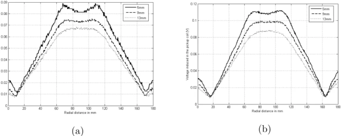
Figure 3.9: Measurement results of Bz at different distances from Coil 1 loaded

with the ferromagnetic steel (a) without ferrite and (b) with ferrite.

(a) (b)

Figure 3.10: Simulation results of Bz at different distances from Coil 1 loaded

with the ferromagnetic steel (a) without ferrite and (b) with ferrite.

even though the coil with the ferrite drew 12% less current from the supply. If the gain in Bz due to the ferrite is normalized with current, it will become 39.2%.

This improvement was 29% for the unloaded case. So it is clear that using a ferromagnetic load improves the effect of ferrite on the system. As we expected, the magnitude of Bz in the loaded case is less than Bz shown in Figure 3.6. This

is due to the opposing Bz in the −z-direction created by the eddy currents in the

load. The inductance of the system with the ferrite and the ferromagnetic steel dropped to 24.54 from 80 µH. This drop is reflected to the decrease in Bz as

expected.

(45)

results are consistent with the measurements except for the fact that the valleys in the simulation results are deeper than the valleys in the measurement results. This is due to the averaging of Bz in the measurement since the pickup coil has

finite area. This discrepancy between the measurement and simulation results can be alleviated by reducing the radius of the pickup coil. However, this would require to feed the coil with higher power since the induced voltage in the pickup coil would be smaller and more noisy as the radius of the pickup coil gets smaller.

(a) (b)

with aluminum (a) without ferrite and (b) with ferrite.

(a) (b)

Figure 3.12: Simulation results of Bz at different distances from Coil 1 loaded

(46)

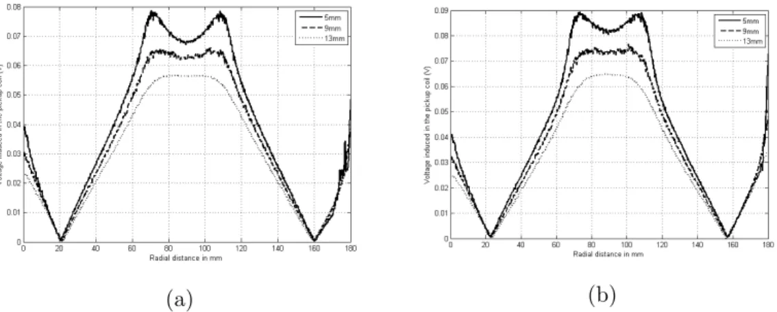
of Bz are shown, respectively, when the coil is loaded with the aluminum. As

seen in these figures, when the coil is loaded with the aluminum, the magnitude of Bz drastically decreases compared to the ferromagnetic steel case. This means

that the electrical loss in the aluminum is less than the electrical loss in the ferromagnetic steel case. Actually, the impedance of the system with the ferrite at 100 kHz when it is loaded with aluminum is 0.578 + j4.76 Ω, whereas it is 9.93 + j15.41 Ω when loaded with the ferromagnetic steel. The inductance of the system is dropped to 7.58 from 24.54 µH. This smaller value of inductance of the system loaded with the aluminum describes why Bz is weaker when the

coil is loaded with the aluminum than when it is loaded with the ferromagnetic steel. Since we drive the system with a constant voltage supply, when the coil is loaded with the aluminum, it draws more current from the supply compared to when the coil is loaded with the ferromagnetic steel. The aluminum load heats up less even though the coil with the aluminum load draws almost 4 times as much current as the coil with the ferromagnetic steel load. This is also apparent in the resistance part of the impedance. This can also be easily seen by comparing the resistive parts of the impedances. When the coil is loaded with the aluminum, the resistance of the system is only 0.578 Ω and in the ferromagnetic steel case it is 9.93 Ω. This shows that heating materials with ferromagnetic properties is more efficient than heating materials without magnetic properties (aluminum, copper, etc.) and apparently this coil will never be able to heat the aluminum.

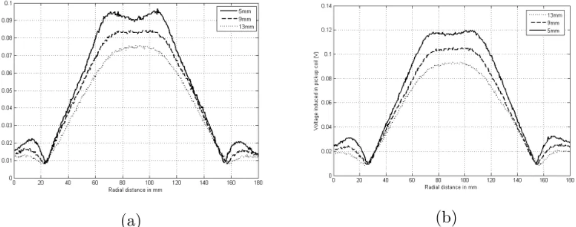
3.1.3 Case study: Coil 2 (rectangular cross-section coil)

The coil we analyzed in this part (Coil 2) is one of the coils (which Bosch uses in its induction ovens). This coil has 26 turns and its outer diameter is 145 mm. In this part we performed the same measurements that we performed for Coil 1 in the previous part. These are unloaded with the ferrite and then without the ferrite, and are also loaded with the ferromagnetic steel and aluminum with and without ferrite. We performed the measurements by driving Coil 2 in the same way as we did Coil 1 in the previous part.

(47)

3.1.3.1 Unloaded Measurements and Simulations of Coil 2

In Figure 3.13, Bz created by Coil 2 is shown. The difference between this coil

and Coil 1 is that the turns in this coil has a rectangular cross section whereas turns in Coil 1 has a circular cross section. Thus, in this coil, more turns could be stacked into a smaller coil diameter. Coil 1 is 180 mm in diameter, although it has fewer turns (24) than Coil 2. This difference in diameters substantially decreases the inductance of Coil 2. Unloaded Coil 2 without the ferrite has an inductance of 50 µH whereas it was 59 µH for Coil 1. So Coil 2 draws much more current than Coil 1 since we feed both coils with a constant voltage source. This difference can be seen when Figure 3.13 is compared with Figure 3.6. Coil 2 creates more Bz than Coil 1 even though the number of turns in both coils is very

close. If it is desired to have a low inductance coil without sacrificing number of turns, the wire crosssection should be chosen rectangular instead of circular so that more turns can be squeezed in less space.

(a) (b)

Figure 3.13: Measurement results of Bz at different distances from unloaded Coil

2 (a) without ferrite and (b) with ferrite.

Figure 3.14 shows the simulation results of unloaded Coil 2. The results are consistent with the measurements. Figure 3.15 shows the all-surface scan of Coil 2. The magnetic field in the z-direction here is symmetric in the φ-direction as expected.

(48)

(a) (b)

Figure 3.14: Simulation results of Bz at different distances from unloaded Coil 2

(a) without ferrite and (b) with ferrite.

(a) (b)

Figure 3.15: All surface scan of Bz at 5 mm above unloaded Coil 2 (a) without

ferrite and (b) with ferrite.

3.1.3.2 Loaded Measurements of Coil 2

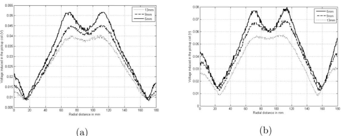
For the loaded analysis, we loaded Coil 2 with the same ferromagnetic steel and aluminum as we loaded Coil 1 with. Figure 3.16 shows the magnitude of Bz

when Coil 2 is loaded with ferromagnetic steel. The value of Bz is much higher

than Bz when using Coil 1. For Coil 2 without ferrite, the peak value of the

induced voltage in the pickup coil is around 65 mV whereas it is 50 mV for Coil 1. This shows that when we drive both coils with the same voltage source, Coil 2 will be able to heat the load better than Coil 1. The same argument holds true for the aluminum load case. As seen in Figure 3.17, the peak value of the induced

(49)

(a) (b)

with ferromagnetic steel (a) without ferrite and (b) with ferrite.

(a) (b)

voltage in the pickup coil is around 45 mV whereas this value for the Coil 1 is around 35 mV.

3.1.4 Case study: Coil 3 (multi-layer, high-turn coil)

The coil we have analyzed in this part is employed for all metal heating purposes in induction ovens (used by Hitachi). By all-metal, we mean coils that are able to heat non-magnetic materials like aluminum and copper. As we have seen in previous analysis, it is hard to heat these metals since they do not enhance the

(50)

magnetic field in the z-direction like ferromagnetic steel does. To heat metals like copper and aluminum, Bz and/or frequency of operation must be increased

so that the time-varying magnetic flux linked to the load is increased. One way of increasing the magnitude of Bz coupled to the load is to use large number of

turns and/or large current values. A smart way of utilizing ferrite also increases Bz.

(a) (b)

Figure 3.18: Pictures of Coil 3 (a) front view and (b) back view.

For this purpose, the coil shown in Figure 3.18 can be used. This coil has an inner radius of 45 mm and an outer radius of 80 mm. Note that this coil is smaller in diameter than Coil 1 we analyzed in the previous part but still has about 40 turns squeezed in three layers. Usual operating frequency of such coils is around 100 kHz. Although this coil is able to heat metals like copper and aluminum the efficiency of this heating is around 30% to 40% whereas the efficiencies for heating a ferromagnetic steel is above 90%.

Figure 3.19 shows the magnitude of Bz when the coil is driven with constant

voltage source at 100 kHz. The coil is unloaded and measurement is taken at a distance of 8 mm above the coil. The impedance of the coil is measured to be 0.77 + j196 Ω. Due to high number of turns, inductance of the unloaded Coil 3 is quite large compared to other coils we analyzed before. It has an inductance of 312 µH whereas it is 59 µH for Coil 1. To heat non-ferromagnetic materials,