A Hybrid Classification Model for Digital Pathology
Using Structural and Statistical Pattern Recognition
Erdem Ozdemir and Cigdem Gunduz-Demir*, Member, IEEE
Abstract—Cancer causes deviations in the distribution of cells, leading to changes in biological structures that they form. Correct localization and characterization of these structures are crucial for accurate cancer diagnosis and grading. In this paper, we introduce an effective hybrid model that employs both structural and statis-tical pattern recognition techniques to locate and characterize the biological structures in a tissue image for tissue quantification. To this end, this hybrid model defines an attributed graph for a tissue image and a set of query graphs as a reference to the normal biolog-ical structure. It then locates key regions that are most similar to a normal biological structure by searching the query graphs over the entire tissue graph. Unlike conventional approaches, this hybrid model quantifies the located key regions with two different types of features extracted using structural and statistical techniques. The first type includes embedding of graph edit distances to the query graphs whereas the second one comprises textural features of the key regions. Working with colon tissue images, our experiments demonstrate that the proposed hybrid model leads to higher classi-fication accuracies, compared against the conventional approaches that use only statistical techniques for tissue quantification.
Index Terms—Automated cancer diagnosis, cancer, graph embedding, histopathological image analysis, inexact graph matching, structural pattern recognition.
I. INTRODUCTION
D
IGITAL pathology systems are becoming increasingly important due to the increase in the amount of digitalized biopsy images and the need for obtaining objective and quick measurements. The implementation of these systems typically requires a deep analysis of biological deformations from a normal to a cancerous tissue as well as the development of accurate models that quantify the deformations. These de-formations are typically observed in the distribution of the cells from which cancer originates, and thus, in the biolog-ical structures that are formed of these cells. For example, colon adenocarcinoma, which accounts for 90%–95% of all colorectal cancers, originates from epithelial cells and leads to deformations in the morphology and composition of gland structures formed of the epithelial cells (Fig. 1). Moreover, the degree of the deformations in these structures is an indicator of the cancer malignancy (grade). Thus, the correct identificationManuscript received September 14, 2012; revised November 05, 2012; ac-cepted November 20, 2012. Date of publication November 27, 2012; date of current version January 30, 2013. This work was supported by the Scientific and Technological Research Council of Turkey under the Project TÜBİTAK 110E232. Asterisk indicates corresponding author.
E. Ozdemir is with the Department of Computer Engineering, Bilkent Uni-versity, Ankara TR-06800, Turkey (e-mail: [email protected])
*C. Gunduz-Demir is with the Department of Computer Engineering, Bilkent University, Ankara TR-06800, Turkey (e-mail: [email protected]).
Digital Object Identifier 10.1109/TMI.2012.2230186
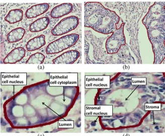
Fig. 1. Colon adenocarcinoma changes the morphology and composition of colon glands. This figure shows the gland boundaries on (a) normal and (b) cancerous tissue images. It also shows the histological tissue components the text will refer to on (c) normal and (d) cancerous gland images.
of the deformations and their accurate quantification are quite critical for precise modeling of cancer.
Although digital pathology systems are implemented for different purposes, including segmentation [1], [2] and retrieval [3], most of the research efforts have been dedicated to tissue image classification. Conventional classification systems are typically based on the use of statistical pattern recognition techniques [4], in which -dimensional feature vectors are extracted to model tissue deformations (i.e., deformations observed in a tissue structure as a consequence of cancer). Dif-ferent approaches have been proposed for feature extraction. The first group directly uses pixel-level information. These approaches employ first order statistics of pixels [5], [6] and/or higher order texture models such as cooccurrence matrices [7], local binary patterns [8], multi-wavelets [9], and fractals [10]. While textural features can usually model the texture of small regions in an image well, they lose the information of local structures, such as the organization characteristics of glands, when they model the entire tissue image.
The second group relies on the use of component-level infor-mation. These approaches extract their features by identifying histological components, mostly cells, within a tissue and quan-tifying their morphology and organization characteristics. Mor-phological approaches quantify the shape and size character-istics of the components [11], [12]. Similar to the textural ap-proaches, they do not consider the organization of the compo-nents in feature extraction. In order to model the organization characteristics, it has been proposed to use structural approaches
that quantify an image by constructing a graph on its tissue com-ponents and extracting global features on the constructed graph [13]–[16]. However, since these global features are extracted over the entire graph, they cannot adequately model the organ-ization characteristics of local structures such as glands in a tissue. More importantly, the extraction of graph features, which are in the form of -dimensional vectors, is only an approx-imation to the entire graph structure and cannot retain all the relations among the graph nodes (tissue components) [17]. On the other hand, structural pattern recognition techniques allow using graphs directly, without representing them by fixed size -dimensional feature vectors [18]. Although such techniques are used in different domains including image segmentation [19], object categorization [20], and protein modeling [21], they have not been considered by the previous structural approaches for tissue image classification. Moreover, these previous ap-proaches have not represented an image as a set of subgraphs that are similar to the query graphs and used them in classifica-tion.
In this paper, we propose a new hybrid model that employs both structural and statistical pattern recognition techniques for tissue image classification. This hybrid model relies on repre-senting a tissue image with an attributed graph of its compo-nents, defining a set of smaller query graphs for normal gland description, and characterizing the image with the properties of its regions whose attributed subgraphs are most structurally sim-ilar to the queried graphs. In order to identify the most simsim-ilar regions, the proposed hybrid model searches each query graph over the entire graph using structural pattern recognition tech-niques and locates the attributed subgraphs whose graph edit distance to the query graph is smallest. It then uses graph edit distances together with textural features extracted from the tified regions to model tissue deformations. Obviously, the iden-tified regions in cancerous tissues are expected to be less sim-ilar to the query graphs than those in normal tissues. Thus, the proposed model embeds the distance and textural features in a -dimensional vector and classifies the image using statistical pattern recognition techniques.
The main contributions of this paper are two-fold. First, it describes a normal gland in terms of a set of query graphs and models tissue deformations by identifying the regions whose subgraphs are most similar to the queried graphs. Second, it embeds the graph edit distances, between the most similar sub-graphs and the query sub-graphs, and the textural features of the identified regions in a feature vector and uses this vector to clas-sify the tissue image. As opposed to the conventional tissue classification approaches, which quantify tissue deformations by extracting global features from their constructed graphs, the proposed hybrid model uses graphs directly to quantify the de-formations. Additionally, it extracts features on only the identi-fied key regions, which allows focusing on the most relevant re-gions for cancer diagnosis (for diagnosis and grading of adeno-carcinomas, these regions correspond to gland structures). The experiments conducted on 3236 colon tissue images show that this hybrid model achieves the highest accuracy compared to the conventional approaches that use statistical pattern recog-nition techniques alone. This indicates the importance of also
using structural pattern recognition techniques for tissue image classification.
II. METHODOLOGY
This paper presents a new approach to tissue image classi-fication. This approach models a tissue image by constructing an attributed graph on its tissue components and describes what a normal gland is by defining a set of smaller query graphs. It searches the query graphs, which correspond to nondeformed normal glands, over the entire tissue graph to locate the at-tributed subgraphs that are most likely to belong to a normal gland structure. Features are then extracted on these subgraphs to quantify tissue deformations, and hence, to classify the tissue. This approach includes three steps: graph generation for tissue images and query glands, localization of key regions (attributed subgraphs) that are likely to be a gland, and feature extraction from the key regions.
A. Tissue Graph Representation
We model a tissue image with an attributed graph where is a set of nodes,
is a set of edges, and is a mapping function that maps each node into an attribute label . This graph representation relies on locating the tissue components in the image, identifying them as the graph nodes, and as-signing the graph edges between these nodes based on their spatial distribution. However, as the exact localization of the components emerges a difficult segmentation problem, we use an approximation that defines circular objects to represent the components.
In order to define these objects, we first quantify the image pixels into two groups: nucleus pixels and non-nucleus pixels. For that, we separate the hematoxylin stain using the deconvo-lution method proposed in [22] and threshold it with the Otsu’s method. Then, on each group of the pixels, we locate a set of circular objects using the circle-fit algorithm [23]. This approx-imation gives us two groups of objects: one group defined on the nucleus pixels and the other defined on the non-nucleus (whiter) pixels1. These groups are herein referred to as “nu-cleus” and “white” objects. Note that in this approximate rep-resentation, there is not always one-to-one correspondence be-tween the components and the objects. For instance, while a nucleus component typically corresponds to a single nucleus object, a lumen component usually corresponds to many white objects forming a clique. Thus, in addition to the types of the objects, their spatial relations are also important for this tissue representation. Graphs can model such relations.
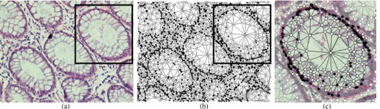
After defining the objects as the graph nodes, we encode their spatial relations by constructing a tissue graph using Delaunay triangulation. For an example image given in Fig. 2(a), the con-structed tissue graph is illustrated in Fig. 2(b) with the centroids
1The second group corresponds to non-nucleus structures including lumens, cytoplasms, and eosin stained stroma regions. Note that it is also possible to define a separate group corresponding to the eosin stained regions. However, since using two object groups is mostly sufficient for effective graph matching, we do not define another object group for the sake of simplicity.
Fig. 2. An illustration of the graph generation step: (a) an example normal tissue image, (b) the tissue graph generated for this image, and (c) a query graph generated to represent a normal gland.
Fig. 3. An illustration of generating a query graph. The node labels are indi-cated using four different representations and the orders in which the nodes are expanded are given inside their corresponding objects.
of the nucleus and white objects (nodes) being shown as black and white circles, respectively.
B. Query Graph Generation
Query graphs are the subgraphs that correspond to normal gland structures in an image. To define a query graph on the tissue graph of a given image, we select a seed node (object) and expand it on the tissue graph using the breadth first search (BFS) algorithm until a particular depth is reached. Then, we take the visited nodes and the edges between these nodes to gen-erate the query graph . In this procedure, the seed node and the depth are manually selected, considering the corresponding gland structure in the image2. Fig. 2(c) shows this query graph generation on an example image; here black and white indicate the selected nodes and edges whereas gray indicates the unse-lected ones.
Subsequently, the mapping function attributes each selected node with a label according to its object type and the order in
2A normal gland is formed of a lumen surrounded by monolayer epithelial cells. The cytoplasms of normal epithelial cells are rich in mucin, which gives them their white-like appearance. Thus, in the ideal case, a query graph con-sists of many white objects at its center surrounded by a single layer nucleus objects. Note that there may exist deviations from this ideal case due to noise and artifacts in an image as well as model approximations, as seen in Fig. 2(c). Subgraphs generated from normal tissues show an object distribution similar to that of a query graph. On the other hand, the object distribution of cancerous tissue subgraphs becomes different since colon adenocarcinoma causes devia-tions in the distribution of epithelial cells and changes the white-look appear-ance of their cytoplasms (epithelial cells become poor in mucin). The graph edit distance features will be used to quantify this difference.
which this node is expanded by the BFS algorithm. In partic-ular, we define four labels: and for the nucleus and white objects whose expansion order is less than the BFS depth and and for the nucleus and white objects whose expansion order is equal to the BFS depth. It is worth noting that the last two labels are used to differentiate the nodes that form the outer parts of a gland from the inner ones and this differentiation helps preserve the gland structure better in in-exact subgraph matching (Section II-C).
The query graph generation and labeling processes are illus-trated in Fig. 3. In this figure, a query graph is generated by taking the dash bordered white object as the seed node and se-lecting the depth as 4. This illustration uses a different repre-sentation for the nodes of a different label: it uses black circles for , white circles for , black circles with green bor-ders for , and white circles with red borders for . It also indicates the expansion order of the selected nodes inside their corresponding circles; note that the order is not indicated for the unselected nodes.
In the experiments, we use four query graphs3generated from four normal images. They correspond to normal gland structures at different orientations. The first column of Fig. 4 shows these query graphs. The query graph generation involves manual se-lection of the seed nodes and the BFS depths, which are selected considering the glands that the query graphs will cover. Note that we also examine the generated query graphs to ensure that they cover almost the entire gland and do not contain any malig-nant structures. The search process for key region localization uses the same algorithm to obtain subgraphs to which a query graph is compared. However, these subgraphs are generated by taking each object as the seed node and selecting the depth as the same with that of the query graph. Thus, the search process involves no manual selection. The search process is detailed in the next section.
C. Key Region Localization
The localization of key regions in an image includes a search process. This process compares each query graph with sub-graphs generated from the tissue graph of the image and
3The number of query graphs affects the number of features to be extracted. Selecting it too small may cause the feature set not to sufficiently represent an image. Selecting it too large increases the number of features, which may de-crease accuracy due to curse of dimensionality. Considering this trade-off, we use four query graphs in our experiments.
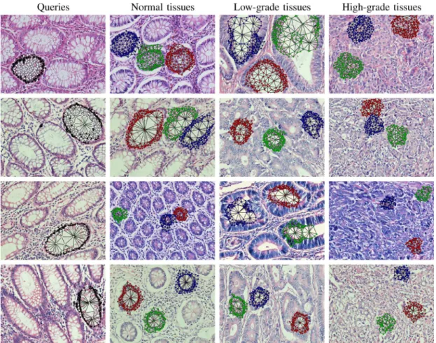
Fig. 4. The query graphs generated as a reference for a normal gland structure and the subgraphs located in example normal, low-grade cancerous, and high-grade cancerous tissue images. The first image of each row shows the query graph on the image from which it is taken whereas the remaining ones show the three-most similar subgraphs to the corresponding query graph. In this figure, the subgraphs of the same image are shown with different colors (red for the most similar subgraph, green for the second-most similar subgraph, and blue for the third-most similar subgraph).
locates the ones that are the -most similar to this query graph. The regions corresponding to the located subgraphs are then considered as the key regions. Since a query graph is generated as to represent a normal gland, the located subgraphs are ex-pected to correspond to the regions that have the highest proba-bility of belonging to a normal gland. Typically, the subgraphs located on a normal tissue image are more similar to the query graph than those located on a cancerous tissue image. Thus, the similarity levels of the located subgraphs together with the fea-tures extracted from their corresponding key regions are used to classify the tissue image.
The search process requires inexact graph matching between the query graph and the subgraphs, which is known to be an NP-complete problem. Thus, we use an approximation together with heuristics on the subgraph definition to reduce the com-plexity to polynomial time.
1) Query Graph Search: Let be a query graph and be its seed node from which all the nodes in are expanded using the BFS algorithm until the graph depth is reached. In order to search this query graph over the entire tissue graph , we enumerate candi-date subgraphs from the graph . For that, we follow a procedure similar to the one that we used to gen-erate the query graph. Particularly, we take each node that has the same label with as a seed node and expand this
node using the BFS algorithm until the query depth . Note that the use of the same BFS algorithm with the same type of the seed node and the same graph depth, which were used in generating the query graph , prunes many possible candi-dates, and thus, yields a smaller candidate set. The nodes of the candidate subgraphs are also attributed with the labels in using the mapping func-tion , which was used to label the nodes of the query graphs (Section II-B).
After they are obtained, each of the candidate subgraphs is compared with the query graph using the graph edit distance metric and the most similar nonoverlapping subgraphs are selected. To this end, we start the selection with the most sim-ilar subgraph and eliminate other candidates if their seed node is an element of the selected subgraph. We repeat this process times until the -most similar subgraphs are selected. For different query graphs, Fig. 4 presents the selected subgraphs in example tissue images; here only three-most similar subgraphs are shown.
Note that although there may not exist normal gland struc-tures in an image, our algorithm locates the -most similar sub-graphs, some of which may correspond to either more deformed gland structures or false glands. In this study, we do not elimi-nate these glands (subgraphs) since the edit graph distance be-tween the query graphs and the subgraphs of more deformed
glands are expected to be higher and this will be an important feature to differentiate normal and cancerous tissue images. In-deed, our experiments reveal that this feature is especially im-portant in the correct classification of high-grade cancerous tis-sues since subgraphs generated from these tistis-sues are expected to look less similar to a query graph, leading to higher graph edit distances. These higher distances might be effective in defining more distinctive features.
Also note that sometimes there may exist normal gland structures in an image but the algorithm may incorrectly locate subgraphs that correspond to nongland benign tissue regions. However, since it locates subgraphs instead of a single one, the effects of such nongland subgraphs could be compensated by the others provided that the number of the nongland graphs is not too much. Otherwise, the localization of these sub-graphs might lead to misclassifications.
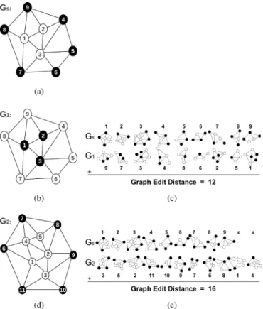
2) Graph Edit Distance Calculation: To select the sub-graphs that are most similar to a query graph , the proposed model uses the graph edit distance algorithm, which gives error-tolerant graph matching. The edit graph distance quantifies the dissimilarity between a source graph and a target graph by calculating the minimum cost of edit operations that should be applied on to transform it into [21], [24]. This algorithm defines three operations: that inserts a target node
into that deletes a source node from
, and that changes the label of a
source node in to that of a target node in . Note that these operations allow matching different sized graphs and with each other. As illustrated in Fig. 4, the proposed graph representation together with this graph edit distance algorithm make it possible to match the query gland regions with the regions of different sizes and orientations.
Let denote a sequence of
opera-tions that transforms into . The graph edit distance is then defined as
(1) where is the cost of the operation . Since finding the optimal sequence requires an exponential number of trials with the number of nodes in and , the proposed model employs the bipartite graph matching algorithm, which is an approxi-mation to the graph edit distance calculation [21]. This algo-rithm decomposes the graphs and into a set of subgraphs each of which contains a node in the graph and its immediate neighbors. Then, the algorithm transforms the problem of graph matching into an assignment problem between the subgraphs of
and and solves it using the Munkres algorithm [25]. This bipartite graph matching algorithm can handle match-ings in relatively larger graphs. However, since it does not consider the spatial relations of the decomposed subgraphs, it may give relatively smaller distance values for the graphs that have different topologies but contain similar subgraphs. This may cause misleading results in the context of our tissue subgraph matching problem. To alleviate the shortcomings of this algorithm, our model proposes to differentiate the nodes
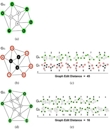
Fig. 5. An illustration of labeling and matching processes used by our pro-posed model: (a) a query graph , (b)–(d) two graphs and that are to be matched with , and (c)–(e) the matches between the decomposed subgraphs of the query graph and the target graphs and . Note that our model uses different attributes for labeling the inner and outer nodes of the same ob-ject type. This helps the matching algorithm better optimize the matching cost, preserving the global structure of a gland.
that form the outer gland boundaries from the inner nodes by assigning them different attribute labels (Section II-B). For example, suppose that we want to match the query graph shown in Fig. 5(a) with two different graphs, and , that are shown in Fig. 5(b) and (d), respectively. In this figure, considering their object types, the graphs and corre-spond to a normal gland whereas the graph corresponds to a nongland region. The bipartite graph matching algorithm with the definition of inner and outer nodes will compute a larger graph edit distance for the - match than the - match; the matches found between the decomposed subgraphs of and the target graphs and are illustrated in Fig. 5(c) and (e), respectively.
Now suppose that we did not differentiate inner and outer nodes for the graphs given in Fig. 5. The corresponding graphs are illustrated in Fig. 6. In this case, the bipartite graph matching algorithm would find similar costs for matching the query graph
with these two graphs, although is more similar to than in our context. This is because of the fact that this al-gorithm matches the decomposed subgraphs of the source and target graphs without considering the spatial relations of these decomposed subgraphs. On the other hand, the differentiation of the inner and outer nodes helps the match algorithm better optimize the matching cost, preserving the global structure of a gland. This mitigates the effects of the aforementioned problem. However, this problem can still be observed among the inner
Fig. 6. The matches between a query graph and two target graphs and when the model does not differentiate the inner and outer nodes.
nodes especially when the BFS depth used in query graph gen-eration is larger; further solutions to this problem are considered as future work.
In this study, we use the unit cost4for graph edit distance cal-culations. The deletion (insertion) operation requires deleting (inserting) a node as well as all of its edges. Hence, the cost
of is where denotes the number
of neighbors of the node . In this cost, the first term cor-responds to the cost of deleting (inserting) a single node and the second one corresponds to the cost of deleting (inserting)
its edges. The cost of consists of two
parts. The first one is the cost of disparity between the labels of and ; hence, it can be denoted as with being the Kronecker delta function. The second part is the cost of matching the edges of and . This cost is defined as where and denote the number of neighbors of and , and denotes the number of their neigh-bors with the same attribute label. In this cost,
corresponds to the cost of matching the edges of and with substitution and corresponds to the cost of deleting
4To match graphs and , the algorithm decomposes them into a set of subgraphs and , and matches the sets using the Munkres algorithm. (Here denotes the subgraph defined for node
by taking and its immediate neighbors.) The total cost of matching and is computed by finding first the disparity cost of matching and and then that of matching their edges. As one end node of each edge is the same ( or ) in the same subgraph, the cost of matching two edges is closely related to the cost of matching their other end nodes. Thus, we use the unit cost for both node and edge disparities. Moreover, we use the same unit cost for all types of node disparities since the use of different costs is not always straightforward. The latter use would increase the number of cost values to be selected, which is more difficult than selecting a single unit cost.
the unmatched edges. Thus, the total cost of substitution is ex-pressed as
(2) Using these cost definitions, the total graph edit distance is cal-culated by summing up the cost of the assignments found by the Munkres algorithm [25].
3) Time Complexity: In this work, we calculate approximate graph edit distances by bipartite graph matching that uses the Munkres algorithm. It is shown that the Munkres algorithm takes time to find the graph edit distance between a source (query) graph and a target
subgraph [21].
To generate a target subgraph from the entire tissue graph , we run BFS starting from a seed node that has the same label with , which is the seed node of the query graph. Thus, for a given image and a query graph, the number of times that the Munkres algorithm is executed is the number of nodes in that has the same label with , which is bounded with . Thus, the time complexity of finding the most similar subgraphs is . Here note that the time complexity of BFS to generate a single target subgraph
is and does not affect the upper
bound time complexity.
D. Feature Extraction and Classification
We characterize a tissue image by extracting two types of local features and classify the image using a linear kernel sup-port vector machine (SVM) classifier [26]. The first type is used to quantify the structural tissue deformations observed in the image. To quantify them, graph matchings are used. However, as a standard SVM classifier does not work with the graphs [27], we embed the graph edit distances of the matchings in a fea-ture vector . To do that, for each query graph , we calcu-late the average of the graph edit distances between this query graph and its -most similar subgraphs selected for the image . Let be a set of the -most similar subgraphs for the query graph . The average graph edit distance for this query graph is
(3) where is the graph edit distance between the query graph and the subgraph . Then, the structural tissue deformations in the image are characterized by defining
the feature vector where is the number
of the query graphs.
The second feature type is used to quantify textural changes observed in the key regions. In our model, we focus on the outer parts of the key regions. The motivation behind this is the fact that changes caused by colon adenocarcinoma are typically ob-served in epithelial cells, which are lined up at gland boundaries. To extract the second type of features, we locate a window on the outer nodes of the subgraphs and extract four simple features on the window pixels that are quantized into three colors using k-means. The first three features are the histogram ratios of the quantized pixels and the last one is a texture descriptor (J-value)
that quantifies their uniformity [28]. Note that the three colors correspond to white, pink, and purple, which are the dominant colors in a tissue stained with hematoxylin-and-eosin. Likewise, we average each of these textural features over the subgraphs of the same query graph. We then put the four average values calculated for each query graph in a feature vector and char-acterize the image using the vector .
III. EXPERIMENTS
A. Dataset
We test our model on 3236 microscopic images of colon tis-sues of 258 patients. Tistis-sues are stained with hematoxylin-and-eosin. Images are digitized at microscope objective lens and pixel resolution is 640 480. Note that after constructing a graph, the magnification and resolution only affect the window size. For larger magnifications and/or resolutions, the window size should be selected large enough so that windows capture sufficient information from the key regions.
Each image is labeled with one of the three classes: normal, low-grade cancerous, and high-grade cancerous. The images are randomly divided into training and test sets. The training set contains 1644 images of 129 patients. It includes 510 normal, 859 low-grade cancerous, and 275 high-grade cancerous tissue images. The test set contains 1592 images of the remaining 129 patients. It includes 491 normal, 844 low-grade cancerous, and 257 high-grade cancerous tissue images.
B. Comparison Methods
We empirically compare our hybrid model against five sets of algorithms. The details of these algorithms are explained in the next sections; their summary is given in Table I. All these algo-rithms except the resampling-based Markovian model (RMM) [29] use linear kernel SVM classifiers; the RMM uses Markov models and voting for classification.
1) Variants of the Proposed Hybrid Model: They include five variants of the hybrid model that we specifically implement to understand the importance of the query graph features used in tissue characterization (first three variants) and the effectiveness of the matching score metric used in subgraph selection (last two variants). The HybridOnlyTextural and
HybridOnlyStruc-tural algorithms use only the texHybridOnlyStruc-tural and strucHybridOnlyStruc-tural (graph edit
distances) features, respectively. We implement them to under-stand the importance of using both of the feature types. The hy-brid model extracts features for each query and concatenates the features of all queries to form a feature vector. On the contrary, the HybridAverage algorithm averages the features instead of concatenating them. We implement it to understand the impor-tance of considering the extracted features on a query base. The hybrid model selects subgraphs with the most similar matching scores. Since query graphs are defined as to represent normal glands, the selected subgraphs are more likely to corre-spond to regions that are most similar to a gland in the image. To understand the effects of this choice, we implement the
Hybrid-Median and HybridDissimilar algorithms that select subgraphs
with the median and the most dissimilar matching scores.
TABLE I
SUMMARY OF THEMETHODSUSED INCOMPARISON
2) Algorithms Using Similar Textural Features: They use the same textural features with the proposed model. However, in-stead of extracting them on the key region boundaries, they ex-tract them in different ways. The RMM [29] generates a set of sequences on an image, uses discrete Markov models to clas-sify each sequence, and classifies the image by voting the se-quence classes. To generate a sese-quence, it first orders the ran-domly selected points and then characterizes them by extracting the four features also used by our current hybrid model. The BagOfWords algorithm also uses the same features to define the words of its dictionary. It divides the image into grids, assigns each grid to the closest word based on the features of the grid, and classifies the image using the frequency of the words that are assigned to its grids. The details of its implementation can be found in [29].
3) Algorithms Using Global Structural Features: They represent an image by constructing a graph on the tissue components and extracting global features on this graph. We implement them to understand the significance of using structural pattern recognition techniques on the constructed graphs. The DelaunayTriangulation algorithm constructs a triangulation on the nucleus components and calculates its global features including the average degree, average clustering coefficient, and diameter as well as the average, standard devia-tion, minimum-to-maximum ratio, and disorder of edge lengths and triangle areas [30]. The ColorGraph algorithm constructs a Delaunay triangulation on the three types of tissue components, colors edges based on the types of their end nodes, and extracts colored versions of global graph features [16].
4) Algorithms Using Intensity and Textural Features: To quantify an image, the IntensityHistogram algorithm calculates features on the intensity histogram of image pixels [31] whereas the CooccurrenceMatrix algorithm extracts features from the
gray-level cooccurrence matrix of the image [32]. The
Gabor-Filter algorithm convolves the image with log-Gabor filters in
six orientations and four scales [33] and averages the responses of different orientations at the same scale to obtain rotation-in-variant features. It calculates the average, standard deviation, minimum-to-maximum ratio, and mode features [30] on the av-erage responses. These three algorithms use the entire image pixels for feature extraction. Their grid-based versions, the
In-tensityHistogramGrid, CooccurrenceMatrixGrid, and Gabor-FilterGrid algorithms, divide a tissue image into grids, compute
their features on each grid, and average them over the image to define their features.
5) Algorithms Combining Structural and Textural Features: Two algorithms are used. The first one combines the Delaunay triangulation and Gabor filter features. We use this combination in our comparisons since these two feature types are frequently used by tissue classification studies [30]. The other combines the features extracted by the color graph and bag-of-words algo-rithms. We combine the features of these algorithms since they give the most successful results on global structural and tex-tural features. Note that we cannot combine the RMM and color graph algorithms at the feature level, since the RMM works on sequences but not on feature vectors.
C. Parameter Selection
Our model has two explicit parameters: is the size of the window that is used to identify the outer parts of the key regions for textural feature extraction and is the number of subgraphs selected by the query graph for a tissue image. Additionally, there is parameter for the linear kernel SVM. In our experiments, we consider all possible combinations
of , and
as candidate parameter sets. Using three-fold cross validation on
the training set, we select , and . For
the other algorithms, we also use three-fold cross validation to select their parameters; the details of the parameters of these algorithms and their selection can be found in [29].
D. Results
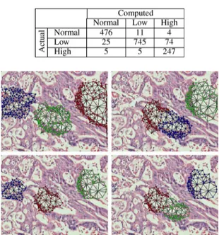
We report the test set accuracies obtained by the hybrid model and the other algorithms in Table II. It shows that our hybrid model obtains higher accuracies for the samples of each class, also leading to the highest overall accuracy. We also provide the confusion matrix for the hybrid model in Table III. As seen in this table, most of the confusions occur in between the low-grade and high-grade cancerous classes. Fig. 7 shows an example of an incorrectly classified image together with the three-most similar subgraphs identified for each query graph. As shown in this figure, some of the identified subgraphs correspond to nongland regions.
Almost all comparison algorithms extract their features on entire tissue pixels of an image. However, this may cause mis-leading results due to the existence of nongland regions in the image, which are irrelevant in the context of colon adenocar-cinoma diagnosis. Moreover, in some images, these irrelevant
TABLE II
TESTSETACCURACIESOBTAINED BY THEPROPOSEDHYBRIDMODEL AND THECOMPARISONALGORITHMS
TABLE III
CONFUSIONMATRIX OF THEHYBRIDMODEL FOR THETESTSET
Fig. 7. An example of an incorrectly classified tissue image. Each image shows the three most-similar subgraphs found by each query graph.
regions may be larger than gland regions, and hence, they con-tribute to the extracted features more than the gland regions. In-stead of using all pixels, the RMM generates multiple sequences from selected points (subregions). However, it randomly se-lects them from the image, without specifically focusing on the gland regions. As opposed to these previous approaches, our hy-brid model uses structural information to locate the key regions, which most likely correspond to gland regions, and extract its features from the key regions. The test results indicate that the
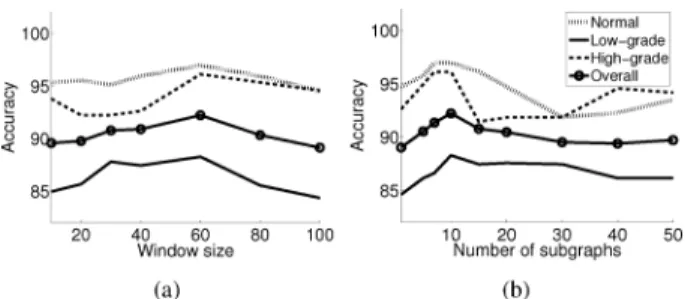
Fig. 8. Test set accuracies as a function of the external model parameters: (a) the window size and (b) the number of selected subgraphs.
feature extraction only from the key regions is effective in im-proving the accuracy.
The hybrid model uses two feature types (structural and tex-tural). To understand the effects of these two feature types sepa-rately, we implement the HybridOnlyStructural and HybridOn-lyTextural algorithms that use only one feature type. The ex-periments show that both algorithms give lower accuracies, in-dicating that the highest accuracies cannot be obtained using only one feature type. Moreover, our model gives better results than the algorithms that combine global textural and structural features, which are defined on the entire image and its graph. This indicates the effectiveness of using local features extracted from the key regions and their corresponding subgraphs. Addi-tionally, when we compare our results with those of the Hybri-dAverage algorithm, we observe that embedding the features of each query separately in a feature vector is more effective than averaging the values for different queries. This indicates that each query and its most similar subregions may give different information, which increases the accuracy.
Table II also shows that the use of the median and the most dissimilar matching scores in subgraph selection decreases the accuracy of the hybrid model, which uses the most similar matching scores. We attribute this accuracy decrease to the following: In the subgraphs with the most dissimilar matching scores, the identified key regions mostly correspond to nong-land regions. In the subgraphs with the median matching scores, the key regions correspond to either gland or nongland regions. Since nongland regions exist in all classes, the effectiveness of the extracted features decreases in differentiating the images of different classes.
E. Parameter Analysis
The proposed hybrid model has two external parameters: the window size and the number of selected subgraphs . Next, we investigate the behavior of our model with respect to these parameters. For that, we change the value of a parameter, fixing the value of the other, and measure the accuracy. Fig. 8 presents the accuracy as a function of and . Here it is worth noting that the number of low-grade cancerous images in the test set is higher than those of the others. Thus, the change in the accuracy of the low-grade cancerous class affects the overall accuracy more than those of the other classes.
The window size affects the size of an area on which textural features are defined. Too small values decrease the accuracy; this is attributed to the fact that the model cannot capture suffi-cient information from the key regions when windows are too
small. When it is selected too large, windows cover a large area and the model becomes similar to the approaches that use en-tire image pixels for feature extraction. In other words, the use of larger window sizes causes to lose locality in feature extrac-tion. This may cause instabilities and decreases the accuracy. Fig. 8(a) presents this analysis.
Fig. 8(b) presents the analysis for the number of the sub-graphs selected by a query for an image. Larger values cause the selected subgraphs to cover an entire image since our model selects nonoverlapping subgraphs. The least similar subgraphs among selected ones may not correctly represent the image, and hence, may lead to instabilities. On the contrary, when only a few subgraphs are selected, the model does not have sufficient information to completely model the image.
IV. CONCLUSION
This work presents a novel hybrid model that makes use of both structural and statistical pattern recognition techniques for tissue image classification. This model proposes to represent a tissue image as an attributed graph of its components and char-acterize the image with the properties of its key regions. The main contribution of this work is on the localization and char-acterization of the key regions. The proposed model uses in-exact graph matching to locate the key regions. To this end, it defines a set of query graphs as a reference to a normal gland structure and specifies the key regions as the subgraphs of the entire tissue graph that are structurally most similar to the query graphs. Then, our model characterizes the key regions using the graph edit distances between the query graphs and their most similar subgraphs as well as extracting textural features from the outer parts of the key regions.
The proposed hybrid model is tested on 3236 colon tissue images. The experiments reveal that this model gives signifi-cantly more accurate results compared to the conventional ap-proaches, which use only statistical pattern recognition tech-niques to quantify the tissue deformations.
One future work is to develop a better approximation algo-rithm for graph edit distance calculations. For example, this al-gorithm may also consider the relations among the decomposed subgraphs. Moreover, one can modify the use of the BFS algo-rithm, or devise a new algoalgo-rithm, in query graph and subgraph construction for more flexible matches.
The hybrid model constructs a tissue graph using Delaunay triangulation, which is known as an effective representation in quantifying spatial relations. However, it is possible to generate graphs through different techniques as future work. For instance, one could assign edges between objects using a probabilistic approach [15]. Alternatively, one could find salient points on an image, characterize these points, and construct a graph on them using Delaunay triangulation.
The model uses four simple features to quantify textural changes of the key regions. Here we selected these features since we also used them in our recent work [29] so that we can make fairer comparisons. Nevertheless, as future work, one can extract more complex features from the key regions, which most probably increase accuracy.
It is possible to adapt the hybrid model to different types of tissues showing different architectures. For that, it is important
to generate query graphs that reflect the architectures of these tissues. For example, for a breast tissue, one could consider defining a set of query graphs as a reference to a normal duct structure. After generating the query graphs, the methodology proposed by the hybrid model can be used. This would be an-other future work of the proposed model.
ACKNOWLEDGMENT
The authors would like to thank Prof. C. Sokmensuer for pro-viding the medical data and the gold standards.
REFERENCES
[1] A. B. Tosun and C. Gunduz-Demir, “Graph run-length matrices for histopathological image segmentation,” IEEE Trans. Med. Imag., vol. 30, no. 3, pp. 721–732, Mar. 2011.
[2] Y. Wang, D. Crookes, O. S. Eldin, S. Wang, P. Hamilton, and J. Dia-mond, “Assisted diagnosis of cervical intraepithelial neoplasia (CIN),”
IEEE J. Sel. Topics Signal Process., vol. 3, no. 1, pp. 112–121, Feb.
2009.
[3] F. Yu and H. H. S. Ip, “Semantic content analysis and annotation of histological image,” Comput. Biol. Med., vol. 38, no. 6, pp. 635–649, 2008.
[4] A. K. Jain, R. P. V. Duin, and J. Mao, “Statistical pattern recognition: A review,” IEEE Trans. Pattern Anal. Mach. Intell., vol. 22, no. 1, pp. 4–37, Jan. 2000.
[5] L. E. Boucheron, Z. Bi, N. R. Harvey, B. S. Manjunath, and D. L. Rimm, “Utility of multispectral imaging for nuclear classification of routine clinical histopathology imagery,” BMC Cell Biol., vol. 8, no. Suppl 1, p. S8, 2007.
[6] A. Tabesh, M. Teverovskiy, H. Y. Pang, V. P. Kumar, D. Verbel, A. Kotsianti, and O. Saidi, “Multifeature prostate cancer diagnosis and Gleason grading of histological images,” IEEE Trans. Med. Imag., vol. 26, no. 10, pp. 1366–1378, Oct. 2007.
[7] S. Doyle, M. Feldman, J. Tomaszewski, and A. Madabhushi, “A boosted Bayesian multi-resolution classifier for prostate cancer detec-tion from digitized needle biopsies,” IEEE Trans. Biomed. Eng., vol. 59, no. 5, pp. 1205–1218, May 2012.
[8] O. Sertel, J. Kong, H. Shimada, U. V. Catalyurek, J. H. Saltz, and M. N. Gurcan, “Computer-aided prognosis of neuroblastoma on whole slide images: Classification of stromal development,” Pattern Recognit., vol. 42, no. 6, pp. 1093–1103, 2009.
[9] K. Jafari-Khouzani and H. Soltanian-Zadeh, “Multiwavelet grading of pathological images of prostate,” IEEE Trans. Biomed. Eng., vol. 50, no. 6, pp. 697–704, Jun. 2003.
[10] P.-W. Huang and C.-H. Lee, “Automatic classification for pathological prostate images based on fractal analysis,” IEEE Trans. Med. Imag., vol. 28, no. 7, pp. 1037–1050, Jul. 2009.
[11] W. Wang, J. A. Ozolek, and G. K. Rohde, “Detection and classifi-cation of thyroid follicular lesions based on nuclear structure from histopathology images,” Cytometry Part A, vol. 77A, no. 5, pp. 485–494, 2010.
[12] C. Wittke, J. Mayer, and F. Schweiggert, “On the classification of prostate carcinoma with methods from spatial statistics,” IEEE Trans.
Inf. Technol. Biomed., vol. 11, no. 4, pp. 406–414, Jul. 2007.
[13] A. N. Basavanhally, S. Ganesan, S. Agner, J. P. Monaco, M. D. Feldman, J. E. Tomaszewski, G. Bhanot, and A. Madabhushi, “Computerized image-based detection and grading of lymphocytic infiltration in HER2+ breast cancer histopathology,” IEEE Trans.
Biomed. Eng., vol. 57, no. 3, pp. 642–653, Mar. 2010.
[14] M. Jondet, R. Agoli-Agbo, and L. Dehennin, “Automatic measure-ment of epithelium differentiation and classification of cervical intra-neoplasia by computerized image analysis,” Diagnostic Pathol., vol. 5, no. 7, 2010.
[15] C. Demir, S. H. Gultekin, and B. Yener, “Learning the topological prop-erties of brain tumors,” IEEE ACM Trans. Comput. Bioinf., vol. 2, no. 3, pp. 262–270, 2005.
[16] D. Altunbay, C. Cigir, C. Sokmensuer, and C. Gunduz-Demir, “Color graphs for automated cancer diagnosis and grading,” IEEE Trans.
Biomed. Eng., vol. 57, no. 3, pp. 665–674, Mar. 2010.
[17] H. Bunke and K. Riesen, “Graph classification based on dissimilarity space embedding,” in Proc. 2008 Joint IAPR Int. Workshop Structural,
Syntactic, Stat. Pattern Recognit., Orlando, FL, 2008, pp. 996–1007.
[18] H. Bunke, “Graph matching: Theoretical foundations, algorithms, and applications,” in Proc. Vis. Interface, Montreal, Canada, May 14–17, 2000.
[19] A. Noma, A. B. V. Gracianoa, R. M. Cesar, L. A. Consularo, and I. Bloch, “Interactive image segmentation by matching attributed rela-tional graphs,” Pattern Recognit., vol. 45, pp. 1159–1179, 2012. [20] D. Macrinia, S. Dickinson, D. Fleet, and K. Siddiqi, “Object
catego-rization using bone graphs,” Comput. Vis. Image Understand., vol. 115, no. 8, pp. 1187–1206, 2011.
[21] K. Riesen and H. Bunke, “Approximate graph edit distance computa-tion by means of bipartite graph matching,” Image Vis. Comput., vol. 27, p. 950, 2009.
[22] A. C. Ruifrok and D. A. Johnston, “Quantification of histochemical staining by color deconvolution,” Anal. Quant. Cytol. Histol. vol. 23, pp. 291–299, 2001 [Online]. Available: http://www.dentistry. bham.ac.uk/landinig/software/cdeconv/cdeconv.html
[23] A. B. Tosun, M. Kandemir, C. Sokmensuer, and C. Gunduz-Demir, “Object-oriented texture analysis for the unsupervised segmentation of biopsy images for cancer detection,” Pattern Recognit., vol. 42, no. 6, pp. 1104–1112, 2009.
[24] D. Conte, P. Foggia, C. Sansone, and M. Vento, “Thirty years of graph matching in pattern recognition,” Int. J. Pattern Recognit. Artif. Intell., vol. 18, no. 3, pp. 265–298, 2004.
[25] J. Munkres, “Algorithms for the assignment and transportation prob-lems,” J. Soc. Indust. Appl. Math., vol. 5, no. 1, pp. 32–38, Mar. 1957. [26] C.-C. Chang and C.-J. Lin, LIBSVM: A Library for Support Vector Machines 2001 [Online]. Available: http://www.csie.ntu.edu.tw/ cjlin/libsvm
[27] B. Luo, R. Wilson, and E. Hancock, “Spectral embedding of graphs,”
Pattern Recognit., vol. 36, no. 10, pp. 2213–2230, 2003.
[28] Y. Deng and B. S. Manjunath, “Unsupervised segmentation of color-texture regions in images and video,” IEEE Trans. Pattern Anal. Mach.
Intell., vol. 23, no. 8, pp. 800–810, Aug. 2001.
[29] E. Ozdemir, C. Sokmensuer, and C. Gunduz-Demir, “A resampling-based Markovian model for automated colon cancer diagnosis,” IEEE
Trans. Biomed. Eng., vol. 59, no. 1, pp. 281–289, Jan. 2012.
[30] S. Doyle, S. Agner, A. Madabhushi, M. Feldman, and J. Tomaszewski, “Automated grading of breast cancer histopathology using spectral clustering with textural and architectural image features,” in Proc.
Biomed Imag.: From Nano to Macro, 2008, pp. 496–499.
[31] M. Wiltgen, A. Gerger, and J. Smolle, “Tissue counter analysis of be-nign common nevi and malignant melanoma,” Int. J. Med. Inf., vol. 69, pp. 17–28, 2003.
[32] A. N. Esgiar, R. N. G. Naguib, B. S. Sharif, M. K. Bennett, and A. Murray, “Microscopic image analysis for quantitative measurement and feature identification of normal and cancerous colonic mucosa,”
IEEE Trans. Inf. Technol. Biomed., vol. 2, no. 3, pp. 197–203, 1998.
[33] P. Kovesi, Code for convolving an image with a bank of Log-Gabor fil-ters [Online]. Available: http://www.csse.uwa.edu.au/ pk/Research/ MatlabFns/PhaseCongruency/gaborconvolve.m