Order quantity and pricing decisions in linear cost inventory systems

r; ? f!

n i n s t r;!s;:;2 CEEiSfiES

m

L£i:i

u m m m m i m i a

A

r

;

esis

S’J*S1TT53 TO T!I2 E*PAilTSE»T OF INDUSTRIAL ENGSREERIHG

013 THE K S m iECF ENGINEESifSa

AND

SCIKJCE

C? SiKENT UNIVStSiTY

1.1 p fa v M m n i v m r

of

the

sstumEMEHTS

FDR THE DEGREE OF

COGTOR C? ?K!L033PKY

L i a U s P ^ i a i s S l u

''W.

I certify that I have read this thesis and that in my opinion it is fully adequate, in scoj^e and in quality, as a dissertation for the degree o f Doctor o f Philosophy.

Prof. Dr. Mahmut Parlar

I certify that 1 have read this thesis and that in my opinion it is fully adequate, in scope and in quality, as a dissertation for the degree o f Doctor o f Philosoj)hy.

Ai)|)roved for the Institute o f Dngiiieering and Science:

P/df. Dr. Mehmet B^jp^y,

ORDER QUANTITY AND PRICING DECISIONS IN LINEAR

COST INVENTORY SYSTEMS

A THESIS

SUHMi r'rED 'I'O 'I'lIE DEPARTMENT OF INDUSTRIAL ENGINEERING AND THE INSTITUTE OF ENGINEERING AND SCIENCE

OF BILKENT UNIVERSITY

IN PARTIAL FULFILLMENT OF THE REQUIREMENTS FOR THE DEGREE OF

DOCTOR OF PHILOSPHY

By

L. Ilakan Polatoglu December 1992

Z

9 2

Нѣ

Цо

. f b S

W

2

с , i

Ь

I certify that I have read this tliesis and that in my opinion it is fully adequate, in sco|)e and in quality, as a dissertation for the degree o f Doctor o f Philosophy.

Prof. Dr. Mahmut Parlar

I certify that

1

have read this thesis and that in my opinion it is fully adequate, in scope and in quality, as a dissertation for the degree o f Doctor o f Philosoi)hy.

Apiuoved for the Institute of Engineering and Science:

P/cif. Dr. Mehmet

1 certify that I have read this thesis and that in my opinion it is fully adeciuate, in scope and in quality, as a dissertation for the degree o f Doctor o f Philosophy.

A ssd cT ^ o f. Dr.

6

emal Dinçer (Supervisor)

I certify that I have read this thesis and that in my opinion it is fully adequate, in scope and in quality, as a dissertation for the degree of Doctor of Philosophy.

1 certify that I have read this thesis and that in my opinion it is fully adequate, in scope and in quality, as a dissertation for the degree o f Doctor o f Philosophy.

1

certify that

1

have read this thesis and that in my opinion it is fully adequate, in scope and in quality, as a dissertation for the degree o f Doctor of Philosophy.

Abstract

ORDER QUANTITY AND PRICING DECISIONS IN LINE AR

COST INVENTORY SYSTEMS

L. Hakan Polatoglu Ph.D. in Industrial Engineering

Supervisor: Assoc. Prof. Dr. Cemal Dinger

January 1993

The primary concern o f this study is to reveal the fundamental characteristics o f the linear cost inventory model where price is a decision variable in addition to procurement quantity. In this context, the optimal solution must not only strike a balance between leftovers and shortages, but also simultaneously search for the best pricing alternative within the low price high demand and high price low demand tradeoff. To some extent, this problem has been studied in the literature. However, it seems that, there is a need to improve the model in order to understand the decision process better. To this end, optimal decisions must be characterised under a more general problem setting than it has been assumed in the existing models. In this study, we employ such a general model.

The overall decision problem can be formulated under a dynamic programming structure. It follows that, the single period model is the basis o f this periodic decision model. For this reason, we concentrate first on this problem. Having characterised the optimal solution to this basic model we extend the decision model to account for the multi-period setting.

It is established with the results o f this study that the decision problem in question is understood better. It is found that the characteristics o f the optim al decision under the proposed model can be substantially different from the properties o f the optim al solution of the corresponding classical model where there is no pricing decision. The primary reason for this is the fact that when there is a shortage in any period, the price that is set in this period could affect the future revenue which must be accounted in the overall decision problem. That is in a general model, price is an information which has an economic value that is transferred from one period to another just like transfering inventories or backlogs to future periods.

Contents

C o n te n ts i

List o f F igu res iii

List o f T ables iv

1

I n t r o d u c t io n an d L ite ra tu re R e v ie w

1

2 S in g le P e r io d M o d e l

5

2.1 Basic Model and Assum ptions...

5

2.2 Mathematical M o d e l ...

6

2.2.1 Optimization P r o b le m ...

7

2.2.2 Existence P r o b le m ... 10 2.2.3 Unimodality ... 12 2.2.4 Optimal S o lu tio n ... 13 2.3 Special C a s e s ... 13 2.3.1 Deterministic M o d e l ... 13 2.3.2 Additive M o d e l... 15 2.3.3 Multiplicative M o d e l... 18 3 M u lt i-P e r io d M o d e l 22 3.1 Mathematical M o d e l ... 23 3.2 Special C a s e s ... ... . 26 3.2.1 Case I ... 26 3.2.2 Case II 27 3.2.3 Case 1 1 1 ... 28 3.3 Deterministic D e m a n d ... 29 3.3.1 Special Case 1 ... 29

3

.

3.2

Special Case I I ...

33

3.3.3 Special C<ise 111... 3.4 Probabilistic Deiiiaiul ...

3.4.1 Optimal Procurement Policy

3.4.2 liiiiiiite Horizon M o d e l... 49 4 N iiiiierica l E x a m p les ₅₃ 5 C o n clu s io n s ₆₉ A p p e n d ix A ₇₄ A p p e n d ix B ₇₇ A i)p e n d ix C ₇₉ A i)p e n d ix D ₈₀ A p p e n d ix E ₈₁

List of Figures

4.1 ICxpecled pseudo-profit function of the second period which is evaluated for Ccises 11 and 13 under the additive uniform distribution and the exponential expected demand function with a = 150, b = 0.5 and a = 0.9...

53

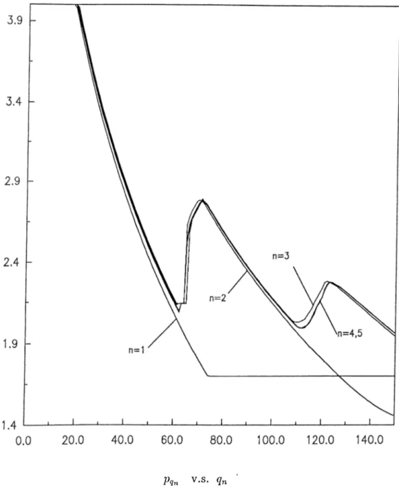
4.2 Expected pseudo-profit curves which are evaluated for a 5-period lost-sales model under an additive uniform demand distribution with c =

0

.

5

, s = 0.25, h =

0

.

01

, tC — 15, A = 20, a == 150, b = 0.5 and a = 0.9...

64

4.3 Best price curves, which gives the optimal values o f pricing decision, for case 13 evaluated under the additive uniform distribution and an exponential expected demand function with a = 150, b = 0.5 and a = 0.9... 65 4.4 Close-uj) of Figure 4.3...

66

4.5 Expected pseudo-profit functions A'/

2

(

0

, P

2

, </

2

) evaluated for case 13 under the additive uniform distribution and an exponential expected demand function with a = 150, b = 0.5 and a = 0.9. The curves are obtained for values o f CO, 62, 64, 65, 70 and 75... 67 4.6 JCxpected j)seudo-profit curves evaluated for 15 periods under the multiplicative

exponential demand with exponential expected demand function. The curve at the top represents the theoretical infinite horizon expected pseudo-profit. Parameters are: c = 0.5, s = 0.25, li = 0.3, 1C = 8y a = 150, b = 0.5, a = 0.7, Ft = 0.1 and Pu = 4.0...

68

List of Tables

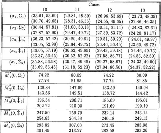
4.1 13 diirerent parameter combinations... 58 4.2 Oi)timal solutions for dilTerent 5-period lost-sales problems. Top values are

evaluated under the additive uniform distribution and bottom ones under the additive triangular distribution both with an exponential expected demand function. Static parameters are: = 0.1, = 4.0, a = 0.9, a = 150, b = 0.5. . 59 4.3 Optimal solutions of the 5-period lost-sales problem solved for cases 10 through

13. The values are evaluated under the additive uniform (top values) and the additive triangular (bottom values) distributions with an exponential expected demand function. The static parameters are: Pi — 0.1, Pu = 4.0, a = 0.9, a = 150, b = 0.5... 60 4.4 Optimal solutions of the

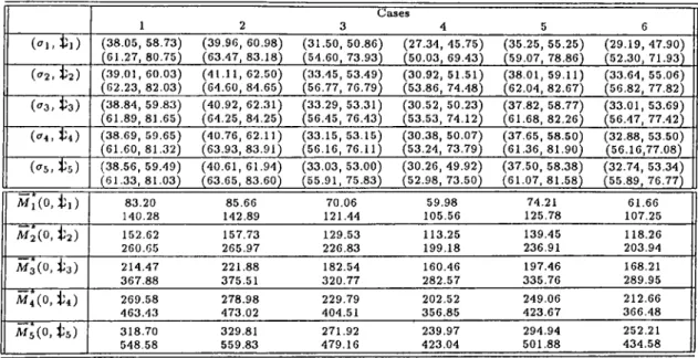
5

-period lost-sales problem that is solved under the

additive uniform distribution for C

2

^es 1 through

6

. The top and bottom values, respectively, are evaluated under an exponential and a linear expected demand functions. The respective functional parameters (a,

6

) are: (150,0.5) and (150,32.5). Other static parameters are: P¿ = 0.1, Pu = 4.0, a = 0.9. . . . 61 4.5 Values o f the critical inventory levels which determine the feasible values

that the optimal control parameters can assume. These values are evaluated under the additive uniform distribution (top values) and the additive triangular distribution (bottom values), with exponential expected demand function. The static parameters are: P¿ = OA, Pu = 4.0, a =

0

.

9

, a = 150, b = 0.5... 62 4.6 Optimal solutions of the 5-period lost-sales problem that is solved under the

multiplicative exponential distribution for cases

1

through

6

with exponential expected demand function. The static parameters are: = 0.1, = 4.0, cv = 0.9, a = 150, 6 = :0 .5 ... 62

Chapter 1

Introduction and Literature

Review

Reorder point, order quantity inventory models are essentially short term planning models. By assumption, the ordering policy does not change the demand pattern or the price structure in the market place during the planning horizon. This cissumption is approximated in a perfectly competitive market where there is no pricing decision to make for the individual vendor. However, there may be incentives for the vendor to increase inventories and wait until the most profitable point in time, if the price is expected to rise in the future; or to clear inventories, if the price is expected to decline. Under imperfect competition, the individual vendor excercises a degree o f monopoly power in the market. He may set a price for his product but then he faces a demand level, governed by some probability distribution, the expected value o f which is decreasing in price. In this context, in addition to the procurement decision, the vendor is confronted by a simultaneous pricing decision.

The simplest model for the study of optimal procurement and pricing decisions is a single- product, periodic review pure inventory model. The planning horizon is divided into review periods which are linked by period ending inventory levels. The vendor is assumed to have full information about costs and demand distributions that are applicable to all periods of the horizon. At the beginning of a review period, given the inventory position (on hand plus on order minus backorders), his problem is to determine the procurement and pricing policies which jointly maximize the expected present value of total profit during the planning horizon.

It hcis been a common practice in demand modeling to express random demand as a combination o f expected demand and a random term. The former has some form of price dej)endency while the latter is price independent. A number o f special cases o f this model have been studied in the literature. These differ, essentially, in the way the demand process

CHAPTER 1. INTRODUCTION AND LITERATURE REVIEW

is represented. In the additive model, Xn{p) = Xn{p) *f where Xn{p) is the demand during period n when the ])rice is p, Xn{p) = /i/'[A'n(p)] and

7

i =

1

,

2

, . . . are independent random variables with E[en] =

0

. in most studies, it is also assumed that A^(p) is nonincrecising in p and, without loss of generality, Xn{p) = A^(p), n =

1

,

2

, . . . . In the muliiplicaiive model, ^n{p) - Xn{p)'en whore E[en] -

1

. In the riskless model, Xn{p) = Xn{p) so that demand in any period is represented by its expected value. This latter case serves both as a first order approximation and as a benchmark for the probabilistic versions of the model.

Whitin [15] appears to have been the first to link price theory and inventory control in a one-period model. Demonstrating that a higher profit level could be achieved for the proposed model, comi)ared to the newsboy problem, he claimed that decision making would be improved by taking j)rice as a control variable.

Mills [7] formalized Whitin’s intuitive approach by studying a one-period inventory model (no holding or shortage costs) with additive demand. He showed that under demand uncertainty the optimal price is less than the optimal riskless price. Mills [7,

8

] also studied the multi-period (infinite horizon) model for which the optimal price was found to be less than that of the one- period model. In addition, he demonstrated that the difference between the optimal starting stock and the expected demand evaluated at the optimal price is greater for the multi-period model.

Later, Karlin and Carr [3] provided a more general inventory model. For both static (one- period model with unit holding and shortage costs) and dynamic (infinite horizon multi-period lost-sales model without holding or shortage costs) cases they studied the optimal decision variables under additive and multiplicative demand, and derived the necessary conditions for optimality. 'I'hey showed, under reasonable assumptions, that the optimal price is greater (less) than the riskless price for the multiplicative (additive) demand for both static and dynamic models.

Nevins [9] provided an empirical study of a special infinite horizon multi-period lost-sales model. He employed the multiplicative demand model with a linear expected demand function under the additional assumptions of a noiidecreasing quadratic procurement cost function, a constant unit inventory holding cost and no shortage cost. For various problem data, he observed that there exists a stochastic equilibrium in which expected demand evaluated at the optimal price equals to the optimal procurement, and there is a tendency that equilibrium inventory level is preserved. However, it appears that Nevins^ definition o f equilibrium inventory is erroneous. Expected sales rather than expected demand should be employed in this definition.

Zabel [18] attempted to provide analytical support to Nevins’ empirical findings. For the one-period model with multiplicative demand, he demonstrated, under some restrictive conditions, the existence of the equilibrium inventory level. Following Nevins’ definition, he showed that the equilibrium inventory level decrecises as holding cost is increased as observed

CHAPTER 1. INTRODUCTION AND LITERATURE REVIEW

by Nevins. Zabel also stated tlie conditions that guarantee the existence and uniqueness of the optimal solution. In a later paper [19], he showed that stronger conditions are needed to guarantee a unique optimal price for the first period of a two-period problem. In addition to the multiplicative demand, Zabel [19] also considered an additive demand model which is slightly different from Mills’ [7] definition. For this model, he demonstrated that under some restrictive cissumptions the optimal values of the decision variables at each period are unique. Moreover, comparing additive and multiplicative demand cases, Zabel concluded that the former tends to yield lower prices and higher inventory levels than the latter. The major source of this characteristic difference is seen as the variance of demand. For the additive model, the variance is constant and for the multiplicative model it is a decreasing function o f price. Therefore, higher prices in the latter model are less risky.

Thowsen [13] formulated a finite horizon multi-period model under additive demand which incorporates partial backlogging. He derived suHlcient conditions under which the optimal procurement is determined by a single critical number policy. He showed that these conditions are satisfied for the case with linear expected demand function and a P F2 distribution for the random term.

Young [IG] represented the random demand as a combination o f the additive and multiplicative models. For the one-period problem, he stated the sufficient conditions under which the optimal starting stock level is unique. Comparing the results with those of the riskless model, he also showed that, if the coefficient o f variation o f demand is nonincreasing in price, then the riskless revenue exceeds the marginal procurement cost at optimality. The converse is true if the variance o f demand is nondecreasing in price. Moreover, correcting Zabel’s [18] definition of equilibrium. Young demonstrated the existence o f an equilibrium inventory level under his assumptions. In addition. Young [17] also studied the infinite horizon multi-period lost-sales problem under his demand model. Assuming that the unsold inventory at the end of each period has an economic value that is equal to the present worth of its procurement cost, he showed that the periods could be separated from each other and the optimal solution could be obtained from the analysis of one-period model.

It appears that Mills’ [

8

] and Karlin and Carr’s [3] approaches establish the conceptual framework of the general inventory model. Nevins’ [9], Zabel’s [18, 19], Thowsen’s [13] and Young’s [16, 17] studies, however, concentrate mostly on the existence and uniqueness o f the optimal solutions for various special cases of the general model. It is demonstrated by these studies that seriously restrictive assumptions on the form o f the expected demand function, on the demand distribution or on the structure of the expected loss function are needed to provide analytical results on the cited issues. In this regard, the existing studies fail to provide a complete understanding of the form of the optimal policies due to analytical intractability.

CHAPTER 1. INTRODUCTION AND LITERATURE REVIEW

isolate the elFects of uncertainty in the context of the theory of the firm. The disadvantage of this rc])resentation, however, is the structural restrictions it brings into the model. For instance, the additive model is restricted by a price-independent (constant) variance. Also it allows negative demand unless the price values are bounded from above. The multiplicative model implies the curious restriction that the demand equals to the product o f its expected value and a random term. As a result of this, variance of demand is the square of its expected value times the variance of the random term. Therefore, variance decreases at a rate faster than expected value and it ai)proaches to zero at high prices.

We believe that there is a need to study the model under general demand uncertainty. It is essential to reveal the fundamental properties of the model independent o f the demand pattern. Especially, uniqueness conditions for optimality must be studied in a more general setting. In this study, we attempt to develop and analyze the model under a general demand uncertainty.

In the classical multi-period inventory model, the proportion of the shortage which is backlogged to the next period is determined by the partial backlogging function. In our model, on the other hand, backlogging needs additional consideration due to the pricing decision. This fact is often ignored by the existing models either by assuming a lost-sales model or by making simplifying assumptions about the forgone revenue due to shortages. In our model, however, we introduce a special relationship (bargaining) between the vendor and the customer over the price that is charged for the backlogs.

In wliat follows, we introduce the single period model in chapter 2. Then, in chapter 3, we study the multi-period model. Chapter 4 provides some numerical examples on the theoretical issues which are discussed in the first three chapters. Finally, in chapter 5 we conclude our findings.

Chapter 2

Single Period Model

In this cliaj)ter, we study the optimal procurement and pricing decisions in a single product one-period pure inventory system. We view this model as a building block of the multi-period model and attempt to establish its cliaracteristics to this end.

2.1

Basic M odel and Assumptions

In this model, the vendor is to make the best procurement and pricing decisions to maximize his profit prior to the beginning of the period. Inventory level before ordering is i. The amount procured, if any, is q — i. A random demand X{p) occurs during the period and at the end o f the period the inventory level is reduced to q — X(p). We consider the case where i > 0. For i < 0, the one-period problem is initiated with an unknown history. That is, the following questions can not be accounted for unless we make assumptions: (1) What fraction of the backlog do we have to satisfy? (2) At what price should we sell that fraction? (3) Do we deduct the backlog from the actual demand or not? These questions will be referred to later in the multi-period model.

We assume that inventory costs are proportional to the period ending inventory level. We denote the unit holding, shortage and procurement costs by /i, s and c, respectively. We also denote the fixed ordering cost by /C. In addition, we assume that, the price is bounded from below and above by Fi and Fu^ respectively, which are the price floor and price ceiling in a regulatory environment. If there are no price regulations, then we consider the price range of (0, oo). We also assume that Fu > c so that it is possible to make profit by retailing.

It follows from the discussion in [

6

] that a way of incorporating price and uncertainty in demand is through an implicit relationship of the type:

CHAPTER 2. SINGLE PERIOD MODEL

where e: is a random term with a known probability distribution. Assuming that T has continuous partial derivatives we may express the random demand as:

X = x {p, e) . (2.1)

Note that the additive and the multiplicative demand models are special forms o f (2.1). We assume that demand distribution, F(a:;p), is defined over x G ( “ Oo, oo) and p G [Pty Pu] such that for all p G [Piy Pu] we have E{Xi{p)]p) =

0

and F { X2(p)]p) =

1

, where Xi{p) and X2{p) are the lower and upper bounds on A (p ), respectively, which are differentiable functions o f p and 0 < A"i(p) < X2{p) < oo. We shall restrict our analysis only to the continuous demand CcLse, bearing in mind that a similar one exists otherwise.

We assume that the expected demand exists (finite), and it is determined from

__ r ^2{v) roo

X { p ) = x-f{x; p)-dx = / [i-F{x-, p)] -dx, (2.2)

Jxdp) Jo

where f{x\p) is the demand density function. We assume that X{p) is a monotone decreasing function of p on (

0

, oo) (if p is confined to [P^, P^]^ then we extend X{p) on (

0

, Pi) and (Pu, oo) by appropriate functions to satisfy the requirements without loss of generality). Moreover, we require that X{p) is o ( l /p ) as p

0

"^ and p —> cx^. This implies that the function pX {p ) starts at zero, first increases and eventually dies away. This function, which is denoted by /i(p ), is called the riskless total revenue by Mills [

8

]. R(p) is a positive valued, finite and differentiable function, which plays an important role in model development. It is shown in Appendix A that R{p) is pseudoconcave on (

0

,oo) when X{p) is either a concave or convex decreasing function; it is also indicated that Il{p) is not pseudoconcave for all monotone decreasing X{p) functions. We assume that R{p) is unimodal; hence, there exists a unique finite price which maximizes P ( p ) .

It is intuitive tliat, in a ‘Tair’^ market, the probability that demand is less than the given level X, P (x ;p ), increases as the price increases. That is,

0F{x;p)

dp

> 0

VxG ( Ai(p) , A

2

(p)). (2.3) It is worthwhile to note that condition (2.3) is sufficient for the requirement that X{p) is a decreasing function of p:

dp

> 0 ^

dX{p)

dp _{= - /} dp •dx <

0

. (2.4)

2.2

Mathematical Model

In this section we develop and analyze the mathematical model under probabilistic demand for the determination o f the optimal price and the beginning inventory level.

CHAPTER 2. SINGLE PERIOD MODEL

2.2.1

Optimization Problem

Coiisidoriiig Uio roi)rosoi)tci(.ioiis iiitrotlucocl iii Section

2

, tlie profit function can be expressed as;

U{p,q) = M{p, q) - I C - 6 { q - i ) ,

where (5(·) is the Heavysidc function and

M(p q) = 1 ~ “ ^ (^(P) - </)> 7 < ^ (P ) < M p), [ p-X(p) - C-(q - i) - h {q - X{p)), ;Ci(p) < X(p) < q, is the pseudo-profit function. We can write the expected profit as:

n(p, q) = £;[II(p,,;)] = M{p, q) - X.6{q - i), where (2.5)

(2.6)

(2.7)

(

2

.

8

)

M{p,q) = E[M{p, i)] = p-X{p) - c-{q - i) - L{p,q).

The first term in (2.8) is the riskless total revenue function. The second term is the procurement cost. The last term is the expected loss function which is given by

L{p,q) = h- { q - x ) - f { x - , p ) dx + {p + s)· {x - q)·f{x\p)-dx ''xtM

(2.9)

= (p + * ■ ) · (p) - '/ ] + (p + s + h)-Q{p, q),

where

0

(p, </) is the expected leftovers i.e.,

/

9 q

(q - 3:)-/(x;p)-dx = I F{x\p)-dx.

We assume that &(p,q) is differentiable in p for </ > 0. Also, we observe that &(p,q) satisfies

(2.10)

0(P . q) > max{0, q - X(p)}, (2.11)

and it is a convex, non-decreasing and differentiable function of q for a given p. Moreover, condition (2.3) implies that

d&iP,q) ^ n dF{q;p)

dp Jx\(_Rp) dp dx >

0

,

*Aii allernalive representation o f &{p,q) is

Q(p,q) = l^q(p) + Q - X(p)]/2,

where A<^(p) is the total expected deviation of demand from g at a price level of p wliich is defined as: r^2{p)

^<l(p)= / ¡X - ql-/(^;p)-dx > 0. dxi(p)

CHAPTER 2. SINGLE PERIOD MODEL

for all ( /€ A"

2

(p)).

From (2.8) and (2.9) it follows that

M{}>, q) = p-[q - Q(p, '/)] - c (q - i) - h-Q{p, q) - s-[X(i») ~ (q ~ Q(p, ?))].

(2.12)

Therefore, M{p^q) is the expected net revenue, less the procurement cost, less the expected holding cost, and less the expected shortage cost. At the expense of loosing intuition about its terms, we shall refer to M{p^q) in what follows in the following form :

A/(p, = (i^ -f 5 - c)^q - s-X{p) - (p + s -f /i)-0 (p , q) + c-i. It is clecir that, M{p^q) is continuous in p on [P^, and in q on [0,oo).

Now, the optimization problem becomes

n(p*.

9

*) = m ax{II(p, q) ; q

6

[i, oo), p

6

[Pr. Pu]}, p,q

(2.13)

(2.14)

where p* and (/* are the optimal values of the decision variables p and q. For this problem we define the suboptimal function

M*(<

7

) = m ax{M (p, g) : p G \Pt, P „]} = M(pg,q), (2.15) where pg is the maximizer. Therefore, M (q) traces the best price trajectory over the q range. Moreover, since M{p,q) is continuous in p and (/, it follows from the Envelope Theorem that M {q) is a continuous function of q (see Appendix B for a proof).

In analyzing (2.14) and (2.15), we need to consider first and second degree partial derivatives o f M{p^q) with respect to p and (/, which cire given by

... ...

dp

d M (p, q)

Op

i ~ 0 (p .

9

) - (p + S + /»)·

dp

0^M{p,q) C>p

2

0H4{p, q)

OpOq

„ i/‘'*A'(p)

„

0Q{p,q)

,

,

x

0'^Q{p,q)

(2.16) (2.17) = 1 - F{q·, p) - (p + S + h)

0F{q-,p)

dp

0M{p,

9

)

Oq

d'^M{p,q)

Oq^

= (

p

+

s

-

c

) - (

p

+

s

+ /

i

)-F(9;

p

),

= -(p + s + /i) ·/(<?;?) <

0

.

(2.18) (2.19)

From (2.19) we conclude that M{p,q) is g-concave on (0 ,o o ), which refers to the newsboy problem setting. On the other liand, (2.16) implies that pj is independent of the procurement

CHAPTER 2. SINGLE PERIOD MODEL

cost. Ill other words, the vendor is to maxiinize his expected profit given that he starts the period with q units. The price dependence of M (p, </), however, is not clear from (2.16) or (2.17).

There is a critical question about the existence of if the price limits are abolished, that is when p E (0,oo). Since,

lim X{p) = oo and lirn X(p) = 0,

/>—

>0

foo Xi{p) and X2{p) must satisfy:

and

lim X\{p) = lim X2(p) = oo,

p—►O p-*0

lirn Xi(p) lirn X2(p) =

0

.

p-*oo p-^oo

Under this setting, it is true that E (0 ,oo)

3

p i,p

2

G (0 ,oo) such that X2{P2) ^

<7

< ^ i(p i)· Therefore, from (2.16) we obtain

and 0M{p,q). dX{p) w N / dX{p) ^\v>V2 — 7"” ·^— ---q + X{p) + {p + s l i ) · dp dp = ^ (p ) + (p +

/0

dp dXjp) dp ■

Moreover, it follows from Corollary A

1

in Appendix A that for p > P/,, X(p) + (p + h) · dX{p)/dp < 0. Thus, we have

9M{p,q)

\p>max{p2,PK} < and there exists a solution pq if there were no price limits.

If Pq is independent of q (a boundary point solution or a constant), then it follows from (2.19) that M (q) is concave at that q. However, if E (P^,Fu), then it must satisfy the first order condition dM{p, q)/dp\p^ =

0

and the second order condition d^M{p^ q)/^P^\pq < for a given q. Since M (p, q) has continuous partial derivatives, we can perform implicit differentiation on the first order condition to obtain

^ 1 - - iP^ + s + h)-dF{q-,p)/dp\p^

20

)

dq -d^M{p,q)/dp\^

ill which the denominator is always positive. Depending on the value of Pq and the price dependency of F{-\p) function, however, the numerator can be positive or negative. Thus, the sign of dpqfdq is not clear.

CUAPTEll 2. SINGLE PERIOD MODEL ₁₀

Since dp^/dq exists, we can write the first derivative of M (q) as

dM jq) _ dM{p^,q) dM{p,q) dp^

dq dq dp dq (2.21)

If Pg e (Pi,Pu), then dM{p,q)/dp\p^ =

0

otherwise dp^fdq =

0

. Therefore, in all combinations o f right-hand and left-hand derivatives the .second term in (

2

.

21

) vanishes. Consequently, we get

dM (q)

dq

= (Pi + s - c) - (p, -h s -1-

h)-F{q\Pg).

Ill order to interpret (2.22) we rewrite it as follows:

dM {q)

dq = {Pq + « ) · [ ! - P'{r,Pq)] - h-P{q;pg) - c.

(2.22)

(2.23)

If the vendor administers his profit maximizing price as he starts with a stock size of then F{q;pg) represents the probability that there will be no shortage. It follows from (2.23) that M {q) increases in q at a rate of (pg + s ) if there is a shortage with probability [1 ’-F{q;pg)] and dccrea.ses at a rate o f li with probability F{q; pg) when there is no shortage. In addition to these two possibilities, M (q) decreases at a rate of c due to tlie procurement cost. Thus the vendor can increase his profit by stocking more given that he is short. When he is short any increase in q will pay him Pg for the sale o f a unit and s for not being short of that unit. Intuitively, the vendor should follow a pricing strategy which will simultaneously minimize F{q]Pg) and keep Pg as high as possible. There is a tradeoff, however, since F{q\pg) increases in pg.

2.2.2

Existence Problem

Intuitively, M (q) must have a peak on [0,oo). However, the existence of this point or, if it exists, its location are not immediately clear. In the following analysis, we shall identify two

——A

separate regions of q in which M (q) is monotone, then we shall prove the existence of its peak. L e m m a 1. V(/ E [0, A’i(Pti)], M (q) is a linear increasing function of q and pg = Pu·

P r o o f. Vr/ E [0 ,^ i(P u )] we have F{q;pg) = 0. Therefore, from (2.10), 0 (p ^ ,i) = 0 and from (2.13) we obtain :

M (q) = nvdx{{p + s - c)’q - s-X{p)+ c-i : p E [Pi, Pu]]

= {Pu + s - c)-q - s-X(Pu) + c-i.

(2.24)

which is a linear increasing function of q and pg = P^.

Lemma 1 indicates that, if we are sure that demand will exceed our stock, i.e. if (/ < Xi{Pu), then we should charge the customers at the highest rate because we not only reduce shortages ill this way but we also incur the maximum unit profit.

CHAPTER 2. SINGLE PERIOD MODEL ₁₁

If X i (/^u) =

0

, tlien the region indicated in Lemma

1

disappears and we loose the information —★

about the slope o f M (q) at q = 0. To account for this possibility, considering (2.22) and the fact thcit 0 < F{q\Pq) < 1 we obtain :

- (/i -f c) < < (Pv + ^ c)> (2.25) which gives the lower and upper limits of the rate o f change of expected profit with respect to the beginning inventory level. It is now clear from (2.24) and (2.25) that at r/ = 0, M^{q) increases at the maximum rate o( Fu -l· s — c.

L em m a

2

. G ^ {^l) ^ linear decreasing function of q and pg is a constant. P r o o f. For q > X-ziPt) we have F{q\Pg) = 1. Therefore, from (2.10), ©(p^,^) = g — X{pg) and from (2.13) we obtain

m""{q) = m a x {(p T /0 * X (p ) : p ^ [Pt, Pu]} - {c + h ) ^ q c - i

= {Fk + h)-X{Fk) - ( c + /i)*g + c-i, (2.26)

where Fh = min{max{P/i, P/:), Pu) and P/^ is the maximizer of the pseudoconcave function (p-f/i)-A ^(p).

We now establish the existence of q, where q = m ax{M {q) : q G [0 ,oo)}. T h e o r e m 1. 3q G {Xi{Pu)i X2{Pi)) M (q) < M [q) Vq G [0,oo).

P r o o f, lly Lemma 1, M {q) is a linear increasing function of q on [

0

,X i(P t

4

)] with a slope of {Fu + s — c) > 0. By Lemma 2, M (q) is a linear decreasing function of q on [XziFi)^ oo) with a slope of —(c-f- /¿) < 0. From (2.25), (P^ -f s — c) and —( c -f h) are the largest and the smallest possible slopes o f M (q), respectively. The proof follows.

Therefore, q must satisfy the first order optimality condition on M (q) which can be obtained from (

2

.

22

) as :

r>- -4- — n

(2.27) n r . p , }= I ’ l l . I

Pq -r S -{- n

The right hand side o f (2.27), RIIS, is a concave increasing function oipg. It becomes negative for Pg < c — s. It follows from (2.22) that, for those Pg values M (q) is decreasing, thus q can not be realized at any price level less than c — s. Alternatively, for pg > c — s, IIIIS attains values between 0 and 1, and we always have a solution for q given such RIIS.

In his pioneering work [15], Whitin brings an intuitive approach to condition (2.27) for a similar decision problem. First, he introduces two conflicting factors: expected profit and expected loss. According to his construct, the expected profit from adding an additional unit to inventory is equal to unit profit times the probability of selling that unit, plus the avoidance of goodwill loss per unit times the same probability, i.e.,

[1

— P(g;pg)]*(pç — c) +

[1

— P(^;Pç)]-s. On the other hand, the expected loss resulting from adding the extra unit is equal to the probability of not selling the unit during the period multiplied by the unit loss from liquidation,

ClIAPTEH 2. SINGLE PERIOD MODEL ₁₂

i.e., F(q;p^)-{h + c). He then argues that if profits are to be maximized, then the expected jirofit obtainable througli stocking an additional unit must be equal to the expected loss, that is;

[1 - F{q]P^)]-iPg + s - c ) = F{q-,p^)-{h + c), which is equivalent to (2.27).

It is possible to construct an upper bound on q by employing the Markov Inequality and condition (2.27). To this end, defining p = pg we write

ttu z l

= i-(i; ji) >

1

-

=

5

.,- < ,№

+ . + '■) X(P)

p + s + /l /l + c

which implies

q < j^-m-<i.x{{p + s + h)-X{p) : p e [ P i , P u ] } , _(2.28) where the maximization problem can be solved for a given X{p) function and the data. Markov Inequality usually yields weak bounds, nevertheless, (2.28) can be useful especially in numerical procedures.

2.2.3

Unimodality

Unimodality of M {q) enables us to identify an ((t, ^ ) type policy which may be employed in determining the optimal q. Moreover, in the multi-period extension of the theory, this becomes an important issue related to the dynamic decision problem.

If Pg G {Pif Pu)j tben differentiating (

2

.

22

) with respect to q we obtain

Noting that dF(q;p,) _ dq — fiQiPq) + dF{q\Pg)

I

dp, dp dq we rewrite (2.29) as d^M^'iq) d^M{p, q) (2.29) (2.30) (2.31)

First term in (2.31) is always positive and the second is always negative. However, their relative magnitudes are not clear. Thus, convexity o f M (q) is not evident from (2.31).

Note that, F(q;p^) is a function o f q only, where F(q;p^) = 0 for 0 <

5

< Xi(Fu) and F{q]Pq) — 1 for X2{Pi) < <i· Therefore, F{q\Pq) has to rise from 0 to 1 between minimum and maximum possible demand values. Meanwhile, it is clear from Lemma 1 and 2 that pq should decrease from P^ to Pi^. If these changes occur rnonotonically, then there will be a unique first order q, which satisfies (2.27). That is, if dF{q;pq)/dq > 0 and dpq/dq < 0, then from (2.29) it

CHAPTER 2. SINGLE PERIOD MODEL ₁₃

follows that M (q) is concave. However, we can state a weaker condition by noting that, it is suincicnt to have dpgfdq < 0 at q = q, provided that dF(q;pg)/dq > 0 Vq. That is.

>

0

and

clq dq

Moreover, from (2.2Ü) and (2.27) we obtain

. <

0

M {q) is uiiimodal. di 0E{q;p). > h-\- c (2.32) (2.33) dp (p + s + li)'^ ’

and we can employ (2.33) in (2.32). On the other hand, we realize that for unimodality of M (q) it is necessary and sufficient to have

d'^M*{q)

dq^ l , <

0

. (2.34)

— K

Uniinoclality of M {q) means once the expected profit of the vendor starts declining at some starting stock level ((/), then he will not be able to avoid this fall by procuring more and incurring the best price. In this case, demand being sensitive to price responds to the veiidor^s profitability. This concept can be related to the degree o f monopoly power of the vendor (Mills [

8

] also mentions this connection without any further detail), however, this is beyond our interest and we leave that discussion open.

2.2.4

Optimal Solution

If M {q) is unirnodal, then from (2.14) it follows that q^ can be determined by an (cr, ^ ) type policy operating on M (q), where n: ^ and a = min{f; : M (q) = M (^ ) — /C}. Consequently, the decision rule is if i < cr otherwise q^ = /, and / / = argmax{M (p, q*) :

2-3

Special Cases

In this section, first we consider the deterministic demand model (the n

5

Â:/e

55

model introduced by Mills [7]) and establish its relation to the probabilistic model. Then, we analyze the additive and the multiplicative models. We provide the relationships that exist between the optimal prices of these models. Finally, under linear expected demand (X{p) = a — b-p^ where a

,6

> 0 and c < I\ < a /

6

), we prove the unimodality of M {q) for uniformly distributed additive e and for exponentially distributed multiplicative e.

2.3.1

Deterministic Model

In this part, we use the subscript “r” to denote the functions and variables of the riskless model. If there is no uncertainty in demand, then we have X{p) = X{p)· Under this specialization.

CIIAPTEli 2. SINGLE PERIOD MODEL 14

leftovers are given by 0 r(p, «z) = niax{0, r /— X (p )}, which is a continuous function. It is, however, non-cliiferentiable at the trajectory given by q = >V(p).

In tlie following discussion, first we prove that M*[q) is unimodal, then we determine the optimal values of the decision variables, and finally we compare the deterministic and probabilistic prolit functions.

T h e o r e m

2

. M*{q) is quasiconcave in q on [0,oo).

P r o o f. For q < X{Pu) we have &r{p, <l) = 0. Thus, from Lemma I it follows that M*{q) is a linear increasing function of q and = P,,.

For X{Pu) < <I we define p such that X{p) — rnin{(Z, A''(Pe)}. Therefore,

i

0

, P i < p < p

© r ( p . ? ) = < (2.35)

[ <

7

- A (p ) , p < p < Pu­ ll nder this .setting, by Lemma 1 we have

argm ax{M r(

7

.>, q) : Pt < P < P) = P, which implies that

M*{q) = m ax{M p(p,q) : p < p < Pu}, where Mr can be obtained from (2.13) and (2.35) as:

^r{p,<l) = { P+ h)-X{p) - ( c + h)-q + c-i.

We note that (p + h ) ' increasing on [Pc,P/,] and decreasing on [Ph,Pu]· Moreover, q < X { P h ) ^ P > h

-It follows from the above discussion that

( P u + s - c ) -

3

-s -A :(P u ) + c-r , q < XiPu),

M*{q) = { p - c)-q + c-i _{, X { P u ) < q < X { P h ) ,} (2.36)

—(c+li) -q + { P h h ) - X { P h ) + c-i , X ( P h )

q-Corollary A3 in Appendix A indicates that {p — c)-q is a p.seudoconcave function o f q on (X (P „ ), A (P r))· Thus, the result follows from (2.36).

From (2.36) it is also clear that

MriPrJlr) = max{M*{q): 0 < q < oo]

= inax{{p - c)-q : X{Pu) <

q

< X{Ph)} + c-i,

CIIAPTEIi 2. SINGLE PERIOD MODEL 15

The maximaiid in (2.37) is the riskless profit function, which is maximized at Pc. According to Corollary A2 we have Ph < Pc which implies that Ph < Pc^ where Pc = rnin{max{P£, T^u}· Therefore, the maximizer in (2.37) is Pc, and we have pr = Pc and qr = AT(Pc). Since Mr is iinimodal, the optimal procurement quantity is determined by an (cr, ^ ) policy, where

t = X { P c ) , and

a = min{q : M^{q) = Af^(i)) - 1C}.

It is intuitive that ijr = X{pr)i that is we procure up to as much as the demand so that we would not pay any penalty for shortages or leftovers. If cr < z, however, then it is optimal not to order (r/* = i) and under our general setting, q^ need not be equal to A (p*). For this reason, it is interesting to note that, although the demand is deterministic, under the optimal strategy there can be shortages or leftovers.

It also follows from (2.36) that G [P/n Pu]· Thus, if Pi < P^^ then P/» can be considered as a lower limit on price that is determined by the expected demand in the market and the cost of carrying inventories. It is indicated in Corollary A2'that as h gets larger P/» gets smaller. Therefore, greater inventory costs enable the vendor to set lower prices in order to maximize his profit. To be more precise, if the vendor has more stocks than AT(P/i), i.e. i > AT(P/j), then he administers a price of Ph and sells all of his stock. Note that this is a short-term planning decision. For a better business strategy he has to take into account the future beyond one-period.

We have 0 (p , q) > ©r(p, (z) from (2.11). Thus, it follows from (2.13) that M (p, q) < Mr{py q) which implies II(p,

7

) < Hr(p, i^)· Also, comparing M (q) and M^{q) we conclude that M {q) remains below the quasiconcave function M^{q) and approaches it at both tails. Therefore, we make the same or more profit in deterministic demand case than we expect (mathematically) in probabilistic case, which is intuitive.

2

.

3.2

Additive Model

Let G{ ) be the distribution of e, then we have

X € [X, (p), X ’M

^ f e [Xi(p) - X{p), X2{p) - J(p)j,

F{x\v) =

G{x-X{p)),

f{x;p)

= g{x-X{p)),

f i - X { p ) Q(p,<l) = — G(e) JXi ( p) - X( p) •de.

CHAPTER 2. SINGLE PERIOD MODEL ₁₆ dF(x-,p) dp dX{p) dp (2.38) de(p,q) dX{p) - o f - = o'^e{p,q) dp^

Under these observations, (2.16) and (2.17) are given by ~f{p<<l) _ ■ dX{i Op dp and

«

=

«

-

efo,) +

d^M{p,q) _ „ d^Xjp) , dXjp) .... , d^Xjp) (2.39) dp“^ dp^ + ^ - ' - ^ - ^ ( F . p ) + {p + s + h ) . : ^ ^ . F i q - , p ) - ( p + s + / i ) - / ( 'z ; p ) - ^ ^ ^ ^ j . It is worthwhile to note that (2.38) together with (2.4) imply that

dX(p)

<

0

^ dF(x;p)

_>

₀

.

(2.40)

(2.41)

dp " dp

It is clear that ifp , G {Pt, Pu), then it must satisfy the first order condition dM{p, q)/dp\p^ = 0. Evaluating this condition for q = q and considering (2.27) we obtain:

dM{p,q), . / - ^ dX(p),

'\f=<I-Q{P,<l) + { p - c ) —

=

dp

which implies p > c. Moreover, adding and subtracting X{p) in (2.42) we get:

q -

0

(p, q) - X{p) + { J ( p ) + (p - c ) . ^

11

, =

0

.

(2.42)

(2.43)

By definition, 0 (p , g) > <1 — X{p)· Therefore, the expression in the brackets, which is the derivative of the riskless profit function, evaluated at p must be positive. Thus, we conclude that

c < p < Pc. (2.44)

This result was first proved by Mills [7] for a simple model. Karlin and Carr [3] showed that the same conclusion is true for the model we are studying by a different approach.

Next, we shall discuss the conditions leading to unirnodality o f M (g). Considering (2.30) and (

2

.

20

), the sufficient condition (2.32) can be written as:

CHAPTER 2. SINGLE PERIOD MODEL ₁₇ --- --- ,

2

. i ® + (p + » + ; . ) . ; ! ^ ) | , >

0

,

i P q + s + h) - { dX{ p ) / d p) \ ^

(ip

dp

-and dpg

1

,-<

0

fi<p,p)> —

—(/i + c)

(2.45) (2.46) (i'J ' ' (p + s P li)^-dX{p)/dp\^

Note that in (2.45) the sum of first three terms is positive. Thus, if the expression in the brackets is negative (this is true when X{p) is linear or concave), then that condition is satisfied. On the other hand, the necessary and sufricient condition (2.34) is given by:

( :

dX{p) d'^X(p)..

'P + s - H , ' ... ...- P · “ ' )

which implies that the second derivative of the riskless revenue function evaluated at p must be negative.

For a given set o f problem specifications, unimodality can be verified by testing the validity of the above cited conditions. For example, suppose that the expected demand function is linear, where X{p) = a - b-p, a

,6

> 0 and p G [0,a/6] with c < a/b. In addition, to prevent negative demand let us assume that < a/b such that X = X(f^u) -h e > 0 Vc. Since d^X{p)/dp'^ = 0, it follows from (2.40) that d^M{p,q)/dp^ < 0 (this observation is essential in achieving better numerical computation performance) and from (2.45) that dF{q\pg)/dq > 0. Moreover, (2.46) can be writen as:

I ^ A V.

/i

+

c

<

0

O f{q-,p^ '> ---and (2.47) reduces to M (q) is uniinodal <ti> f{q\p) > b-{p + s T h y ' {h

4

- c y (2.48) (2.49) 2 -h-{p+ s + h y '

Clearly, (2.49) is weaker than (2.48). Furthermore, it can be deduced from (2.44) that if

f{<T,p) > {h + cy/[2-b-{c + s + hy], (2.50)

then (2.49) will hold.

For a given distribution and the data the conditions (2.48), (2.49) or (2.50) can be tested. For instance, if

e

has a uniform distribution on [—A, A], then for all

q

G

i ^ i { p ) i ^

2

{p))·

-

2

- A ’

F{q-,p) = q - a + b-p-P X

2 X ’ (2.51)

CHAPTER 2. SINGLE PERIOD MODEL

18

I'rom (2.49) we obtain the condition for unimodality as

A < b {f> + s + or from (2.50) the suilicient condition as

A < b - { c + s + hf/{h + c f .

(2.53)

(2.54) Under tlie proposed special case, we can view A as a measure of demand uncertainty and b as a measure o f sensitivity o f demand o f price changes. From (2.53) we conclude that the less the uncertainty and/or the more the demand sensitivity are, the more unimodality will be favored. An alternative approach is to solve p and q from (2.27) simultaneously under the hypothesis

——A·

tliat M (q) is uniinodal. To this end, we rewrite (2.27) and (2.42), respectively, as:

and

p - h s - c

( / - a - f i - p - f A

^(r.p) = = --- jTj;--- ,

q - 6 ( p , q ) - b - ( p - c ) = 0. Using (2.52) we solve for q:

^p + s + li Next, substituting (

2

.

57

) in (2.55) we get:

P - ^ ^ - ^ r + b i p - c ) .

(2.55)

(2.56)

(2.57)

p + s + A - V A · (2.58)

Since under the additive model p < Pc for a linear expected demand function P^ = (a + b-c)/2b, the term in the square root is always defined. After manipulations we rewrite (2.58) as

p + s - c

=

1

-a + b-c — 2-b-p

2-{p + s - l h f - { P c - p ) - \-{h + cy/b -

0

, (2.59)

which is a polynomial having a local maximum at [2-Pc — (/i+ s )]/3 . It follows that this function has at least one and at most two positive roots. In addition, one of the positive roots is always located in the interval ([2-Pc - (h + s)]/3,Pc)· Since the third critical point, on the feasible price range, to make a local minimum does not exist, we conclude that M (q) is unimodal.

2.3.3

Multiplicative Model

Let G(-) be the distribution of e, then we have

a·· e [A i(p), X2(p)] i e [-Vi(p) /a:(p) ,X2/x (p)],

CHAPTER 2. SINGLE PERIOD MODEL 19 f{x-,p) = g(x/X{p))/Xip), dF{x-,p) i/N(p) (p)/ X{p) d X { p ) X mIX(p) Q{p,<l) = — G{c)-d(, JXi (p)/ X{p) dp dp X (p) de(p,q) _ dXjp) ( ¡ ■F{q; p)-e {p, q) (2.60) dp dp _{x i p )}

d'^e{p,q)

_

d^X(p) q-F{q\p)-

0 {p,q) ^ ( dX{p)__ ^

“ c/p

2

^ dp J(p)^

Under these observations (2.16) and (2.17) are given by:

■f{q\p)·

dp ‘ dp ' d p ^ (p ) and d^Mjp, q) d?X{p) ^ q - F { q ; p ) - e { p , q ) i dX{p) ^ d'^Xjp) . , , , \ dp dp'^ ^ C dpo

2

- = —s--- , dp^ 4"

_x(p)

- (i> + s + /0 -/(7 iP ) / dX(p) (2.62) V X{p)J

Clearly condition (2.41) al.so holds for the multiplicative model.

If Pj € (Ft, Fu), then it must satisfy the first order condition dM{p, q)/dp\p^ = 0. Evaluating (2.16) at pj, setting it equal to zero and arranging terms we get

= r (1 - + (P + op " ^{Pq) — S dXjp), X{Pg)-q-F{q; Pg ) + e{p^,q) _

0

. (2.63) dp X ( p ,)

Since 0 (p , q ) > q - X{p), we have Q(p, q) + X { p ) ~ q-F{q; p) > 0. Thus, the first and the third terms in (2.63) are positive. Moreover, we note that q-F{q\p) - 0 (p , g) > 0. Therefore, (2.63)

implies that __

{>^(í>) + (P + /

0

· ^ ^ ^ } | „

< 0

P q > h -Furthermore, evaluating (2.63) at q and rearranging the terms we obtain

Q(P· <1 X(P)

CHAPTER 2. SINGLE PERIOD MODEL ₂₀

d X j p ) ^^ Xi p) - _q + e{p,q)

(2.64)

x(p)

The second term is positive, since p > P/^, and so is tlie third term. Therefore, we must have

{

+ {p - c) ·

}

1

^ <

0

p > P c > c .

This result is the same as Karlin and Carr’s [3] conclusion, which Wcis proved by a different approach than ours.

Considering (2.30) and (2.20), the sufficient conditions for unimodality o f (2.32), can be written, respectively, as:

«

1

- F ( , ;p, )

+ ^ ± % L

dq

{Pg+s + h)-q

{ p + s + li)-q-{dX{p)/dpy and ^ l

, - < 0

^ f{q-,p)> dp ^ dp^ '' _____- X ( p ) i h + c) (2.65) (

2

.

66

) d q " ' ~ ' ' q-{p + s - P hY-dX{p)/dp\p

The sum of the first three terms in (2.65) is positive. Thus, if the expression in the brackets is negative (that is true when X{ p) is linear or concave), then that condition is satisfied. On the other hand, the necessary and sufficient condition (2.34) is given by:

^ ' + (? 5 + . + / o ■ / ( v ; y ) ■ [ g - e ( p , ? ) ] · | 1 ^ < 0, (2.67)

p -f s T 11 _{X{ p) dX{p)/dp ^}

which implies that the expected demand must be “normal” at p or, equivalently, expected marginal revenue to be decreasing at p.

The above cited conditions can be tested for a given set of problem specifications. For instance, under a linear expected demand assumption, which is described in the previous section, it follows from (2.62) that 5^M(p, q)/dp'^ < 0 and from (2.65) that dF{q\pq)/dq > 0. Moreover, (

2

.

66

) can be written as:

dq h-q-[p + s h y and (2.67) reduces to ---\ · · 11 r/'~ -'X ’ X{ p) M ( , ) ,s uminodal « / ( , ; p ) > 2 .t .[ j - e ( p , , - ) ] . ( p + a + (

2.68)

(2.69)

ClIAPTEli 2. SINGLE PERIOD MODEL

21

If c is exponential, for examj)le, then for all q £ (0,oo);

e - i/ N ( .p )

f{q-,p) =

x(p)

F{q-,p) =

Q{p,<l) = <1- N{p)-F(q;p).

Using these relationships and (2.27), the unimodality condition (2.69) could be written as:

2

-p^ + (3-/i + 4-s- c)-;}-1-2-(s + / 0 - ( 5 -c) - - y { l ı - l · c ) > 0. (2.70) The quadratic form in (2.70) has a critical point at —(3 /i + 4-s — c )/4 which is less than c, hence, it is also less than Pc· Since p > Pc, if

2-P'^ + (3-/i +

4-5

- c)-Pc + 2-(s + li)-{s - c) - - - ( / i -f c) > 0, then (2.70) will hold. After necessary manipulations, (2.71) reduces to

(•^)^ + (/i + 4-s “ c)··^ + (4-s^ + 4-/i-s — /i-c) > 0,

(2.71)

(2.72)

where the critical point of the quadratic form is — (/i + 4-s — c )/2 which is less than c. Since a/b > c under linear expected demand assumption, condition (2.72) can be rewritten гıs:

^ - *[\/(A + c)-(/i + c -

8

-s) - {li +

4-5

-- c)]. (2.73) We note that (2.72) holds when li + c < 8-s (i.e. when the expression in the square root is negative). Otherwise, we observe that

a/b > C- 2- S > ^ -[\ /(/i + c)-(/i -f c - 8-s) - {li + 4-s - c)],

which holds by the natural assumption that a/b > c. Therefore, M {q) is uriimodal for exponcnticil multiplicative demand model. Zabel [18] arrived at the same conclusion, under some restrictions, for the case where s =

0

.

Since pricing decision aifects tlie period ending inventory level, the analysis o f the multi­ period model does not trivially follow from the analysis o f the one-period model. In the next chapter we shall dwell on this issue.

Chapter 3

Multi-Period Model

111

this chapter, we extend the planning horizon more than one period and try to characterize the optimal procurement and pricing decisions. In this regard, before getting into the mathematical model we shall first describe the multi-period setting.

We assume that the planning horizon is divided into N review periods, which are indexed by n. The Icist period, n = l, is the end of the planning horizon. If there are any shortages in this period, they will be lost. Also, we assume that there is no salvage value for the leftovers. At the beginning of each period, the vendor decides how much to order, qn — inj and what price to administer, Pm until the next decision point. is the beginning inventory level before ordering and Qn is the beginning inventory level after ordering in period n. With these decisions, the vendor tries to maximize the mathematical expectation of the sum of current period’s profit and the discounted j)rofit of the remaining periods, which is denoted by Il^j. We assume that In > 0, so that the decision problem is not initiated with an unaccountable debt. For simplicity we assume constant unit holding, shortage, procurement costs and a fixed ordering cost, which are denoted by /i, s, c and A^*, respectively. We also consider a common discount factor for each period and denote it by a. Furthermore, we assume that procurement lead time is negligibly short compared to the length of a period and all payments realize without any significant delay or additional cost.

Let us consider period 7i, where 1 < n < TV. It is clear that depends on and the backlogging rule. Therefore, in any period, except the last one, the pricing decision can not be made independent of the future periods. Moreover, it follows from the analysis of the one-period model that procurement quantity and pricing decisions could not be analytically decoupled. Hence, the overall optimization problem, that is the determination o f optimal procurement quantity and price for all periods, does not follow directly from the classical multi­ period model. In other words, since price is a decision variable which is a factor that affects demand, we need to extend the analysis of the classical multi-period model which employs price

CHAPTER 3. MULTI-PERIOD MODEL ₂₃

only as a unit revenue.

A conceptual complication arises in relation to unsatisfied customers when there is a shortage in any intermediate period. In the classical model, it is customary to assume a backlogging rule which allows all customers to wait another period (full backlogging), some customers to wait another period (partial backlogging) or all customers to quit (lost sales). When there is a pricing decision, however, the willingness of a customer to wait one more period may be contingent upon price. That is, there might be a bargain between an unsatisfied customer and the vendor for their mutual benefit. Therefore, it is likely that such a customer-vendor interaction will affect the optimal solution. To study this, we could employ various backlogging rules in our model. For instance, we may assume that the vendor issues a “rain check” for customers who are willing to wait, provided that they could pay the current price in the future. Under the multi-])criod model that we are studying, we may cissume that, if there is a shortage, then, upon mutual agreement, the customers are to wait until their demand is satisfied regardless of the price; wait as long as they could pay the current period’s price at any time in the future; wait only one period at any price; wait only one period at the current period’s price; or, we may assume that the vendor does not allow backlogging. It is intuitive to expect and it will be clear in the following sections that a backlogging rule induces a special structure into the model. Since a variety of different backlogging rules can be employed, it is difficult to generalize possible vendor-customer relationships without making further assumptions. In fact, this generalization will not be argued in this study. Instead, we shall be analysing the model under three different backlogging rules to demonstrate the characteristic differences between them. Not to complicate the analysis further, it will be assumed that the vendor-customer relationship is homogeneous; that is, there is no difference between the customers, and the vendor is not practicing any price discrimination. It is also assumed that the backlogs are cleared before satisfying the current demand in any period.

3.1

Mathematical Model

Under the proposed assumptions, the expected 7i-period profit can be expressed as a backward dynamic programming recursion:

Un{i,x,PN,PN-U· ■■,Pn,<lti) = Mn{in,PN,PN-l, ■ ■■,Pn,qn) ~ IC-S{qn - in), (3.1) where Mn is the expected n-period pseudo-profit function (i.e., the expected profit regardless of the ordering cost) which will be defined later. II„ is expressed not only as a function of current period’s decision variables, pn and but also in terms o f all previous pricing decision variables which might be employed by a backlogging rule in general. We adopt the convension that if the backlogging rule does not require a subset of the price variables through Pn+ij tlien those