FINITE PERTURBATION ANALYSIS METHODS FOR
OPTIMIZATION OF PERIODIC (s,S) INVENTORY
CONTROL SYSTEMS
A THESIS
SUBMITTED TO THE DEPARTMENT OF INDUSTRIAL ENGINEERING
AND THE INSTITUTE OF ENGINEERING AND SCIENCE OF BILKENT UNIVERSITY
IN PARTIAL FULFILLMENT OF THE REQUIREMENTS FOR THE DEGREE OF
MASTER OF SCIENCE
by Erdinç Mert
ii
I certify that I have read this thesis and that in my opinion it is fully adequate, in scope and in quality, as a thesis for the degree of Master of Science.
____________________________________ Asst. Prof. Dr. Kağan Gökbayrak (Advisor)
I certify that I have read this thesis and that in my opinion it is fully adequate, in scope and in quality, as a thesis for the degree of Master of Science.
____________________________________ Asst. Prof. Dr. Osman Alp
I certify that I have read this thesis and that in my opinion it is fully adequate, in scope and in quality, as a thesis for the degree of Master of Science.
____________________________________ Asst. Prof. Dr. Ayşe Kocabıyıkoğlu
Approved for the Institute of Engineering and Sciences:
___________________________________ Prof. Dr. Mehmet Baray
iii
ABSTRACT
FINITE PERTURBATION ANALYSIS METHODS FOR
OPTIMIZATION OF PERIODIC (s,S) INVENTORY
CONTROL SYSTEMS
Erdinç Mert
M.S. in Industrial Engineering
Supervisor: Asst. Prof. Dr. Kağan Gökbayrak July, 2008
We are dealing with single item inventory systems where the period time is constant and the unsatisfied demands are backordered. The demands are independent and identically distributed random variables, but the distribution of those variables are not known. The total cost of a period consists of; ordering cost "K" which is independent of the ordering quantity, holding cost "h" for each item that remains in stock, and penalty cost "p" for the each backordered item. In the considered system, it is known that when the parameters of an (s,S) inventory policy are chosen appropriate, then the expected period cost can be minimized. There are some exact methods or heuristics for finding the optimal s and S parameters in the literature for the case where the demand distribution is known. In our study, we introduce a perturbation analysis based method for finding the optimal s and S parameters where the demand distribution is not known. Our method anticipates the sensitivity of (s,S) parameters to the period cost for the observed demand quantities. This method's performance is compared with a method that uses Integer Programming with the past data and with a method that calculates the mean and standard variation values with the past data and feeds them to the Ehrhardt's Heuristic.
Keywords: Inventory Policies, Perturbation Analysis, Simulation
iv
ÖZET
DAĞILIMI BİLİNMEYEN RASSAL AYRIK TALEPLER İÇİN
PERİYODİK (s,S) ENVANTER DENETİM METODU
Erdinç Mert
Endüstri Mühendisliği, Yüksek Lisans Tez Yöneticisi: Yrd. Doç. Dr. Kağan Gökbayrak
Temmuz, 2008
Karşılanamayan taleplerin bekletilebildiği ve tedarik zamanlarının sabit olduğu tek öğeli envanter sistemlerini ele almaktayız. Gözlem periyotları içinde gelen talep miktarlarının bağımsız özdeşçe dağılmış ayrık rastgele değişkenler oldukları ancak bu değişkenlerin dağılımının bilinmediği kabul edilmektedir. Her periyot için maliyet, sipariş miktarından bağımsız K sipariş maliyeti, elde kalan her birim için h tutma maliyeti ve karşılanmak için bekletilen her birim talep için p yoksatma maliyeti toplamından oluşmaktadır. Ele alınan sistemde parametreleri doğru seçilmiş (s,S) envanter denetim politikasının beklenen periyot maliyetlerini en aza indirgeyebileceği bilinmektedir. Literatürde talep dağılımın bilinmesi durumunda en iyi s ve S parametrelerinin bulunabilmesi için önerilmiş tam veya sezgisel yöntemler bulunmaktadır. Bu çalışmamızda ise dağılımın bilinmediği durumda, yöntemimizin yakınsamasına yeterli süreler için dağılımın durağan kalacağı kabulu ile, en iyi s ve S değerlerinin bulunması için sarsım analizi tabanlı dağılım değişiklerine uyarlanabilir bir yöntem önermekteyiz. Gerçekleşen talep miktarları için periyot maliyetlerinin s ve S parametrelerine duyarlılıklarını tahmin eden ve bu parametreleri yenileyen yöntemimizin performansı geriye dönük tamsayı programlaması sonuçlarını uygulayan ve gerçekleşen miktarlar için hesaplanan ortalama ve standard sapma değerlerini Ehrhardt sezgiseline besleyen iki yöntemin performansları ile karşılaştırılmaktadır.
Anahtar Sözcükler: Envanter Politikaları, Sarsım Analizi, Simulasyon
v
vi
ACKNOWLEDGMENTS
I would like to express my sincere gratitude to Asst. Prof. Dr. Kağan Gökbayrak for all his attention and supports during my graduate study and for his valuable guidance and most importantly for his patience and trust.
I am indebted to members of my dissertation committee: Asst. Prof. Dr. Osman Alp and Asst. Prof. Dr. Ayşe Kocabıyıkoğlu for showing of kindness to accept to read and review this thesis. I am grateful to them for their effort, sparing their valuable time for me and for their support.
I am most thankful to members of Land and Missile Programs, especially to Mr. Aybars Küçük and Mr. Oğuz Yemişçiler, for their support and their patience. I would like also thank to my friends in Bilkent IE for their friendship.
Finally, I would like to express my deepest gratitude on my family for believing in my work and sacrifices that they have made for me. I feel very lucky to have such a wonderful sister, father and mother. Without their love and support, I would never have finished this thesis.
vii
CONTENTS
1 INTRODUCTION ...1 2 BACKGROUND...4 2.1 Iventory Systems ...4 2.2 Inventory Policies ...5 2.3 Problem Formulation...82.4 Determining Optimal (s,S) Policy Parameters...13
3 PERTURBATION ANALYSIS METHODS FOR OPTIMIZATION OF POLICY PARAMETERS...22
3.1 Perturbation Analysis Algorithms...22
3.1.1 Perturbation Analysis on "s" (Algorithm 1)...23
3.1.2 Perturbation Analysis on "q" (Algorithm 2) ...24
3.2 Finding Optimal (s*,q*) Pair...26
3.3 Initializing Perturbation Analysis Parameters ...29
4 SIMULATION ...34
4.1 Logical Model...34
viii
5 NUMERICAL EXAMPLES ...39
5.1 Poisson Distribution...40
5.2 Comparison with Other Algorithms...44
5.3 Adaptability ...46
6 CONCLUSIONS AND FUTURE DIRECTIONS ...49
REFERENCES ...52
APPENDICES...55
A PA on "s" - Algorithm 1 ...55
B PA on "q" - Algorithm 2 ...56
C Finding Optimal (s*,q*) Pair - Algorithm 3 ...57
D Ehrhardt's Heuristic Code...80
E Flowchart...83
F ARENA Simulation Model...84
G EXCEL Simulation Model ...85
H MATLAB Simulation Model...86
I GAMS Code...91
J Outputs of Numerical Examples ...95
ix
LIST OF FIGURES
4.1 Numerical Example of Inventory Simulation for s=10, S=15 ...36
4.2 Inventory Simulation Example...37
J.1 (s*,S*) Graph for PA Alg. POI(10), γ=ALL HISTORY ...95
J.2 (s*,S*) Graph for PA Alg. POI(10), γ=3 ...95
J.3 (s*,S*) Graph for EHR Alg. POI(10), γ=ALL HISTORY ...96
J.4 (s*,S*) Graph for EHR Alg. POI(10), γ=3 ...96
J.5 (s*,S*) Graph for RIP Alg. POI(10), γ=ALL HISTORY ...97
J.6 (s*,S*) Graph for RIP Alg. POI(10), γ=3 ...97
J.7 Comparison of (s*,S*) Graphs for POI(10), γ=ALL HISTORY ...98
J.8 Comparison of (s*,S*) Graphs for POI(10), γ=3 ...98
J.9 Comparison of Cost Graphs for POI(10), γ=ALL HISTORY...99
J.10 Comparison of Cost Graphs for POI(10), γ=3 ...99
J.11 (s*,S*) Graph for PA Alg. POI(25), γ=ALL HISTORY ...100
J.12 (s*,S*) Graph for PA Alg. POI(25), γ=3 ...100
J.13 (s*,S*) Graph for EHR Alg. POI(25), γ=ALL HISTORY ...101
J.14 (s*,S*) Graph for EHR Alg. POI(25), γ=3 ...101
J.15 (s*,S*) Graph for RIP Alg. POI(25), γ=ALL HISTORY ...102
x
J.17 Comparison of (s*,S*) Graphs for POI(25), γ=ALL HISTORY ...103
J.18 Comparison of (s*,S*) Graphs for POI(25), γ=3 ...103
J.19 Comparison of Cost Graphs for POI(25), γ=ALL HISTORY ...104
J.20 Comparison of Cost Graphs for POI(25), γ=3 ...104
J.21 Comparison of (s*,S*) Graphs for UNI(0,10) ...105
J.22 Comparison of Cost Graphs for UNI(0,10)...105
J.23 Comparison of (s*,S*) Graphs for NOR(5,1) ...106
J.24 Comparison of Cost Graphs for NOR(5,1) ...106
J.25 Comparison of (s*,S*) Graphs for Empirical Distribution ...107
J.26 Comparison of Cost Graphs for Empirical Distribution ...107
J.27 (s*,S*) Graph for PA Alg., δ=15, γ=3 ...108
J.28 (s*,S*) Graph for EHR Alg., δ=15, γ=3 ...108
J.29 (s*,S*) Graph for RIP Alg., δ=15, γ=3 ...109
J.30 Comparison of (s*,S*) Graphs, δ=15, γ=3 ...109
J.31 (s*,S*) Graph for PA Alg., δ=15, γ=ALL HISTORY ...110
J.32 (s*,S*) Graph for EHR Alg., δ=15, γ= ALL HISTORY ...110
J.33 (s*,S*) Graph for RIP Alg., δ=15, γ= ALL HISTORY ...111
J.34 Comparison of (s*,S*) Graphs, δ=15, γ= ALL HISTORY ...111
J.35 (s*,S*) Graph for PA Alg., δ=90, γ=ALL HISTORY ...112
xi
J.37 (s*,S*) Graph for RIP Alg., δ=90, γ= ALL HISTORY ...113 J.38 Comparison of (s*,S*) Graphs, δ=90, γ= ALL HISTORY ...113
1
CHAPTER 1
INTRODUCTION
Inventories are assets held for sale in the ordinary course of business or in the process of production for such sale or supplies to be consumed in the production process or in the rendering of services. Some inventories have to be held due to the lead time of the goods and the ordering cost. Holding inventories in stock causes a cost, holding cost, because of the cost of storage, the opportunity cost, etc. On the other hand, if no inventories are held, the customers cannot find what they want and since the customer is not satisfied, there is a potential for the loss of future orders. Thus, having no inventories will also cause a cost; namely penalty cost. The third type of cost is named as ordering cost and it is the money given for the transportation of the goods, all possible administration tools to place an order, etc.
Inventory policies are methods for determining when and how many units to order in order to minimize an inventory cost function. There are two types of inventory policies; continuous review policies and periodic review policies. In the first type, the inventory position is monitored continuously and when the inventory position falls below a pre-specified level, an order is given. In the periodic review policies, the inventory position is monitored in periods and the same action is taken. One of the periodic review policy is the (R,s,S) policy where the inventory position is checked in every period of R time units and if the inventory position is less than or equal to s, an order is placed to raise the position up to S. The inventory policy discussed in this thesis will be the (R,s,S) policy for given R time units, and the aim is to find the optimal (s,S) values to minimize the expected summation of holding cost, penalty cost and the ordering cost.
1 Introduction 2
The aim is to design inventory control policies for random demand distributions that can adapt themselves to sudden demand changes. For that purpose, Perturbation Analy-sis Algorithm will be de ned and will be compared with two other algorithms; Ehrhardt's Heuristic and Retrospective Integer Programming Method. Perturbation Analysis Algo-rithm is a perturbation analysis based method for nding the optimal s and S parameters. This method will anticipate the sensitivity of s, S parameters to the period cost for the ob-served demand quantities. This algorithm can nd the real optimal s; S parameters without knowing the distribution, mean and the variance of the demand distribution.
Ehrhardt's Heuristic is a simple heuristic that calculates near-optimal (s; S) values by calculating the mean and the standard deviation by the observed data. Retrospective Integer Programming Method also uses the past data and nds the minimum cost by integer programming.
In the second chapter, some background information about the Inventory Systems and Inventory Policies are given. The problem formulation is de ned and a literature review about how to determine optimal (s; S) parameters is mentioned.
In Chapter 3, the main method, Perturbation Analysis, is introduced. At the end of this chapter, methods to nd the optimal (s; S) pair are given.
In Chapter 4, the logical model is de ned, and the simulation models are introduced. Chapter 5 consists of numerical examples. In this chapter, several distributions are taken as the demand distributions and the algorithms de ned in Chapter 3 are tested. Also com-parison of the algorithms (Perturbation Analysis Algorithm, Ehrhardt's Heuristic and
Ret-1 Introduction 3
rospective Integer Programming Method) can be found in this chapter. This chapter ends with the adaptability issue.
The last chapter includes the conclusion and general discussion about the outputs of numerical examples. At the end of this chapter, future directions are given and the thesis ends with the appendices.
4
CHAPTER 2
BACKGROUND
2.1 Inventory Systems
Inventories are assets held for sale in the ordinary course of business or in the process of production for such sale or supplies to be consumed in the production process or in the rendering of services. Fogarty & Hoffman (1983) defines inventory as:
Inventory ties up capital, uses storage space, requires handling, deteriorates, sometimes becomes obsolete, incurs taxes, requires insurance, can be stolen, and sometimes is lost ... the absence of the appropriate inventory will halt a production process; ... an expensive piece of earth moving equipment may be idled by lack of a small replacement part; a patient may die due to the unavailability of plasma; ... and, in many cases, a good customer may become irate and take his business elsewhere if the desired product is not immediately available.
Thus, inventories serve the function of providing a buffer between customer demands and production capabilities (Aft 1987). There are three basic classes of inventories for a company;
• Raw materials are the items that are purchased from another vendor to be processed further.
• Work in process inventories are still not finished goods but processed raw materials.
• Finished goods are the products that are available for sale.
In this thesis, inventory will only represent the "finished goods" which are considered as discrete units.
2.2 Inventory Policies 5
An inventory system is a system in which the following three kinds of costs are signi cant; the cost of carrying inventories, the cost of incurring shortages, and the cost of replenishing inventories (Eliezer 1982). After this part, these costs will be recalled as holding cost, penalty cost, and ordering cost, respectively. Holding cost applies if there is a positive inventory on hand, penalty cost applies if there is unsatis ed order, and ordering cost applies if order was made at that time.
2.2 Inventory Policies
Inventory policies are methods for determining when and how many units to order in order to minimize an inventory cost function. Based on the inventory level, anticipated demand and cost function, these policies answer the following questions:
1. When should the inventory be replenished?
2. How many units should be added to the inventory? (Eliezer 1982) For the rst question, following answers can be given;
Inventory should be replenished when the amount in inventory is equal to or below s quantity units
Inventory should be replenished every R time units For the second question, the answers can be;
2.2 Inventory Policies 6
A quantity should be ordered so that the amount in inventory is brought to a level of S quantity units
If the demand is deterministic, then some methods can be used to nd the answers of these questions. However, if the demand is stochastic, then some inventory policies should be used. The quantities s; R; q; S used above are the policy parameters and de ned as the reorder point, scheduling period, lot size, and order-up-to level, respectively.
Based on the reviewing process, inventory policies are divided into two main groups; continuous review policies and periodic review policies.
2.2.1 Continuous Review Policies
In continuous review policies, the inventory control system is designed so that the inventory position (inventory on hand plus orders given but not received yet) is monitored continu-ously. When the inventory level is suf ciently low, an order is given at that time and the given order is received after a certain lead time. Well known continuous review policies are (s; S)Policy and (s; Q) Policy.
(s,S) Policy
In (s; S) Ordering Policy, whenever the inventory position falls to the reorder point s, an order is placed enough to raise the position to the order-up-to level S:
2.2 Inventory Policies 7
(s,Q) Policy
An (s; Q) Ordering Policy means that when the level of inventory position is less than or equal to s, an order of xed amount of Q is placed.
2.2.2 Periodic Review Policies
Another alternative of Continuous Review is to consider the inventory position only at certain given points in time. The intervals between these reviews are constant and that is called the Periodic Review. Well known periodic review policies are (R; s; S) Policy, (R; s; Q)Policy and (R; S) Policy.
(R,s,S) Policy
In intervals of R time units, the inventory position is checked and if the inventory position is less than or equal to s, an order is placed to raise the position up to S.
(R,s,Q) Policy
In (R; s; Q) policy, the inventory position is checked in every period of R time units and if the inventory position is less than or equal to s, an order of amount Q is placed.
As can be seen easily, in the rst policy, the inventory position is always increased to same value after orders, where in the second policy, always the same quantity of orders are given.
2.3 Problem Formulation 8
(R,S) Policy (Base Stock Policy)
In this policy, an order up to S at the end of each period of R time units is placed, unless the period demand is zero.
In this thesis, Periodic (R; s; S) Policy will be analyzed for a xed and given time period, R. After this part, "(s; S) Policies" will be used for "(R; s; S) Policies" and the aim is to nd optimal s and S values that minimize a total cost. For that purpose, we consider a single-item inventory system where un lled demand is backlogged with a xed lead time Lbetween placement and delivery of an order where the holding cost and penalty cost are linear, and the demand is random.
2.3 Problem Formulation
We have a stochastic inventory control problem with an unknown demand distribution. The demand distribution shall not have any known distribution; the algorithms in this thesis work for all kinds of distributions and also for empirical distributions. There is a non-negative constant lead time and three types of costs (holding cost, penalty cost, and ordering cost). Detailed information of the costs are given below.
Holding Cost: Holding cost applies while holding inventory on stock. Holding in-ventory causes a cost because there is an opportunity cost (money invested in inin-ventory could be placed on bank for interest), storage cost (need for place to store the inventory), deterioration cost (materials deteriorate over time), obsolescence problem (products may become outdated), insurance cost (insurance protects against potential loss), etc.
2.3 Problem Formulation 9
Thus, holding cost is applied if the inventory on hand is positive at the end of the day. The holding cost per unit "h" is multiplied with the "Inventory on Hand", and the total holding cost is calculated.
Penalty Cost: It is also known as stockout cost or shortage cost. There are two types of penalty cost; in the rst type, the customer is willing to backorder and to wait for the delivery, where in the second, customer does not wait and the order is lost. In this thesis, we assume full backlogging. However, it also causes a cost since you cannot satisfy your customer and there is a potential for the loss of future orders (Aft 1987).
Thus, if the inventory on hand at the end of the day is negative, penalty cost is applied. The penalty cost per unit "p" is multiplied by the total "Unsatis ed Demand" at the end of that period and the total penalty cost is calculated. Since backlogging policy is applied, the unsatis ed demand is forwarded to the following day until all of the past demands are satis ed.
Ordering Cost: There are usually xed costs associated with a replenishment (inde-pendent of the batch size). It may be described as a truck with in nite capacity delivering the orders and even if one order is placed, the same money will be given to the truck. Thus, if order is given in a day, Ordering Cost (Set-Up Cost) "K" is also incurred. In other words, this cost is independent of the ordered unit size, i.e. ordering 1 unit and 100 units will have the same ordering cost.
Then, the total cost is de ned as:
2.3 Problem Formulation 10
where Y is the inventory position at the end of the period, X is the inventory level at the end of the period, and I is the indicator function.
2.3.1 Mathematical Model
The model of the problem can be formulated as:
min s;S E[(J = limn!1 1 n n X i=1 Ji)] Ji = IfYi sgK + h max(Xi; 0) + p max( Xi; 0) Xi = Xi 1+ Ri Di Yi = Xi 1+ Oi 1 Di Oi = Oi 1+ Qi Ri Qi = IfYi sg(S Yi) Ri = Qi L 1 X0 = S O0 = 0 Q0 = 0
2.3 Problem Formulation 11
where the problem parameters are as below: Di : Demand Occurred at Period i
L : Constant Lead Time h : Holding Cost per unit
p : Penalty Cost per unsatis ed units
K : Ordering cost for placing an order, independent of number of units s : Inventory control policy parameter, Reorder Point
S : Inventory control policy parameter, Order Up-To Level and the state variables/decision variables of the problem are as below:
Ji : Total Cost at the end of Period i
Yi : Inventory Position at the beginning of Period i
Xi : Inventory Level at the beginning of Period i
Ri : Received Orders at the beginning of Period i
Qi : Order Quantity at the beginning of Period i
Oi : Outstanding Orders at the beginning of Period i
By Inventory Position, we mean inventory on hand plus on order minus backorders. By Inventory Level, we mean inventory on hand minus backorders. Lead Time is the time between the placement of an order and the arrival of that order.
2.3 Problem Formulation 12
For linearizing the problem, the model was rewritten as below:
min Z = X
i
J (i)
J (i) KI1(i) + hX(i)
J (i) KI1(i) pX(i) X(1) = S D(1)
X(i) = X(i 1) + R(i) D(i); for i > 1 Y (1) = X(1)
Y (i) = X(i 1) + O(i 1) D(i); for i > 1 O(1) = Q(1)
O(i) = O(i 1) + Q(i) R(i); for i > 1 Q(i) S Y (i) M (1 I1(i))
Q(i) S Y (i) + M (1 I1(i))
Q(i) M I1(i)
R(1) = 0
R(i) = Q(i L 1); for i > 1 s S
M I1(i) s Y (i) + 1
M I2(i) Y (i) s
2.4 Determining Optimal (s,S) Policy Parameters 13
where
M is a very big number, I1and I2are binary variables,
sand S are integers,
J; R; Oand Q are positive variables.
2.4 Determining Optimal (s,S) Policy Parameters
In this section, the literature about determining the optimal (s; S) inventory policy para-meters will be reviewed. The analysis of (s; S) inventory policies started out as a research topic after the introduction of the multistage periodic review inventory model in the pa-per by Arrow, Harris & Marschak (1951). In that papa-per, they studied uncertainty models–a static and a dynamic one–in which the demand ow is a random variable with a known probability distribution. The best maximum stock and the best reordering point are deter-mined as functions of the demand distribution, the cost of making an order, and the penalty of stock depletion.
Scarf (1960) and Iglehart (1963) showed that an optimal policy can be found within the class of (s; S) policies where there are linear costs, stochastic demand, and a xed lead time. Thus, since our assumptions satisfy these requirements, there will always be an optimal (s; S) policy that minimizes the average cost. However, computing the opti-mal policy that minimizes the long term average cost has become a big problem for years since there are a potentially in nite number of (s; S) combinations. There are mainly two categories for nding the optimal (s; S) pair; exact method and heuristics. Iglehart (1963),
2.4 Determining Optimal (s,S) Policy Parameters 14
Veinott&Wagner (1965), Bell (1970), Archibald&Silver (1978), Federgruen&Zipkin (1984), Zheng&Federgruen (1991), Feng&Xiao (2000) and Daniel&Rajendran (2005) are all ex-amples about the rst category, exact method. On the other side, Naddor (1975), Ehrhardt (1979, 1984) and Roundy&Muckstadt (2000) are the most known papers that introduce heuristics for (s; S) optimization.
Exact Methods (For known demand distribution):
Iglehart (1963) gives bounds for the sequences fsng and fSng and discusses their
lim-iting behavior. The limlim-iting (s; S) policy characterizes the optimal ordering policy for the in nite horizon problem. In Veinott&Wagner (1965), a complete computational ap-proach for nding optimal (s; S) inventory policies is developed. The model is named as a dynamic inventory model in which demands for a single product are independent, identically distributed (i.i.d) discrete random variables. There is a constant lead time, a discount factor 0 1;a xed non-negative set up cost, a linear purchase cost, a con-vex expected holding and penalty cost function, and total backlogging of un lled demand. The objective of the paper is to choose the control parameters (s; S) which minimizes the long run average cost per period. The methods of Veinott&Wagner (1965), Bell (1970), and Archibald&Silver (1978) apply complete enumeration method where it is bounded by lower bounds s, S and upper bounds s, S for nding the optimal values of s and S .
Sahin (1982) analyzes the behavior of (s; S) inventory models. Both for periodic and continuous review systems, Sahin states that for constant lead times and full backlogging, expected cost E(s; ) is convex in s where = S s:From that point, he proves that both
2.4 Determining Optimal (s,S) Policy Parameters 15
for periodic and continuous review systems with full backlogging, constant lead times, and linear holding and shortage costs, E(s1( ); ) is pseudoconvex on 0: After
that, in Federgruen&Zipkin (1984), an iterative algorithm to compute an optimal (s; S) policy under standard assumptions (stationary data, well-behaved one-period costs, discrete demand, full backlogging) is presented. The algorithm starts with a given (s; S) policy and evaluates a sequence of policies, and converges to an optimal one in a nite number of iterations.
In Zheng&Federgruen (1991), a new algorithm for computing optimal (s; S) policies is derived based upon a number of new properties of the in nite horizon cost function c(s; S) as well as a new upper bound for optimal order-up-to levels S and a new lower bound for optimal reorder levels s . In other words, Zheng&Federgruen (1991) propose a simple and ef cient algorithm that searches directly on (s; S) plane. While improving the average cost c(s; S), the search moves vertically up and horizontally right to upgrade the s and S values at each step until reaching the optimal s ; S pair. The algorithm's computational complexity is 2.4 times that required to evaluate a single (s; S) policy and this algorithm can be applied both to periodic review and continuous review inventory systems. Zheng&Federgruen de nes:
D =the one-period demand (random variable); pj = PrfD = jg, j = 0; 1; 2; :::;
K =the xed cost to place an order;
2.4 Determining Optimal (s,S) Policy Parameters 16 G(y) = 8 > > > > < > > > > : Ch y X d=0 (y d) Pr(D = d) + Cp 1 X d=y+1 (d y) Pr(D = d) for y 1 Cp 1 X d=0 (d y) Pr(D = d) for y < 1 After de ning this G function, the long-run average cost c(s; S) is calculated as:
c(s; S) = M (S s)K + S s 1X j=0 m(j)G(S j) where m(0) = (1 p0) 1 M (0) = 0 m(j) = j X l=0 plm(j l); j = 1; 2; ::: M (j) = M (j 1) + m(j 1); j = 1; 2; :::
Feng&Xiao (2000) uses the method that Zheng&Federgruen (1991) introduced, and proposes a new approach to solve the optimal (s; S) inventory policy. A dummy cost factor and an auxiliary function were introduced in this paper. The algorithm searches for the optimal dummy cost through continuously evaluating the auxiliary function.
Daniel&Rajendran (2005) studies the performance of a single-product serial supply chain operating with a base-stock policy and optimizes the inventory levels in the supply to minimize the total supply chain cost with holding and shortage costs. A genetic algorithm is proposed to optimize the base-stock levels with the objective of minimizing the sum of holding and shortage costs in the entire supply chain. Simulation is used to evaluate the base-stock levels generated by the genetic algorithm. The effectiveness of this algorithm is compared with a random search procedure. Optimal base-stock levels are obtained through
2.4 Determining Optimal (s,S) Policy Parameters 17
complete enumeration of the solution space and compared with those yielded by this algo-rithm. It is found that the solutions generated by the proposed algorithm do not signi cantly differ from the optimal solution obtained through complete enumeration for different sup-ply chain settings, thereby showing the effectiveness of the proposed algorithm.
Heuristics (For known demand distribution):
As mentioned before, there are also some papers that introduce heuristics to nd the optimal pair of (s; S). Naddor (1975) derives a heuristic decision rule that computes optimal s and S values. The rule requires the knowledge of the mean and standard deviation of demand, probability of no demand, carrying and replenishing costs, desired availability, and leadtime. Ehrhardt (1979) presents an analytic approximation for computing (s; S) policies for single items under periodic review with a set up cost, linear holding and shortage costs, xed lead time, and backlogging of un lled demand. He calls the approximation as the "Power Approximation". By that approximation, it is very easy to compute the optimal s and S values by only knowing the mean and the variance of the demand.
The Power Approximation is de ned as follows: Let L = (L + 1) and L = p L + 1: Then, qp = 1:463 0:364(k=h)0:498 0:138L ; z = fqp=[(1 + p=h) L]g0:5; sp = L+ 0:832 L ( 2= )0:187(0:220=z + 1:142 2:866z)
2.4 Determining Optimal (s,S) Policy Parameters 18
And if qp= is greater than 1.5, then s = sp and S = sp+ qp. If demands are to be
integer values, sp and qp values are rounded to the nearest integer.
Ehrhardt (1984) introduces the Revised Power Approximation. In Ehrhardt (1979), it is likely that the accuracy of the Power Approximation will suffer when the variance of demand is very small. Thus, a revised version of the Power Approximation is published. The Revised Power Approximation is de ned as follows:
Let L = (L + 1) and L = p L + 1: Then, qp = 1:3 0:494(k=h)0:506(1 + 2L= 2 )0:116; z = [qp=( L p=h)] 1=2 ; sp = 0:973 L+ L(0:183=z + 1:063 2:192z)
Roundy&Muckstadt (2000) study the problem of determining production quantities in each period of an in nite horizon for a single item produced in a capacity-limited facility. The demand for the product is random, and it is independent and identically distributed from period to period. Un lled demand is backordered. A base stock or order-up-to policy is used. They develop a new approximation for this distribution, and perform extensive computational tests of existing approximations. Their new approximation works extremely well as long as the coef cient of variation of the demand is less than two.
2.4 Determining Optimal (s,S) Policy Parameters 19
Retrospective Approaches (If demand distribution is not known):
All of the methods until this part, we had the assumption of knowing the demand distrib-ution or at least the mean and the variance. After this part, some retrospective approaches will be introduced. In Fu&Healy (1992), a periodic review (s; S) inventory system is con-sidered. The problem in this paper considers the inventory control of an item which is measured in continuous units. The in nite horizon problem is considered and simulation is used to nd the optimal s and S values that minimize the average cost per period. The gen-eral assumptions of this paper are; gengen-eral independent and identically distributed (i.i.d.) continuous demands, zero lead time, full backlogging of orders, and linear ordering, hold-ing and shortage costs.
Two approaches are introduced in this paper: a deterministic "retrospective" algo-rithm and a gradient-based, steepest-descent algoalgo-rithm. The more important approach is the second one which involves estimating the gradient of the performance measure of in-terest and adjusting the parameters according to the gradient during the evolution of the simulation. The simulation terminates when the gradient is "close enough" to zero. As L'Ecuyer (1991) states, there are two main techniques for gradient estimation; perturbation analysis and likelihood ratio. Perturbation analysis is a technique for gradient estimation from a single simulation of a discrete-event system.
The perturbation analysis estimators for continuous demand is derived in Fu (1994) and PA algorithms for @J=@s and @J=@q (for continuous demand and zero lead time) are given where J denotes the average cost per period.
2.4 Determining Optimal (s,S) Policy Parameters 20
In Fu (1994), sample path derivatives of performance measures were derived for (s; S)inventory systems. The objective is again to nd optimal s and S values that mini-mize the average total cost. In this paper, nondiscounted periodic review system with i.i.d continuous demands, full backlogging, constant lead time and general holding, shortage costs are considered. The approach is sample path analysis with the focus on sample path derivatives. Since it deals with derivative estimation, the paper assumes that demands take continuous values. Also, in this paper Fu focuses on in nitesmall perturbation analysis (IPA) and smoothed perturbation analysis (SPA) for nding the estimators of s and S.
Fu&Healy (1997) utilizes the perturbation analysis estimators derived in Fu (1994) for zero lead time. In this paper, two approaches (gradient-based methods and retrospective approach) for the optimization of a periodic review (s; S) inventory systems are compared, and a Perturbation Analysis algorithm that combines these two approaches is proposed.
Glasserman&Tayur (1995) develop simulation-based methods for estimating sensi-tivities of inventory costs with respect to policy parameters. They consider capacitated, multiechelon systems operating under base-stock policies and develop estimators of deriv-atives with respect to base-stock levels. They formulate and validate in nitesimal per-turbation analysis derivative estimates for multiechelon capacitated production-inventory systems. It means that they introduce appropriate algorithms and show that they converge to the correct values. The convergence is shown over the number of independent simula-tion runs for derivatives of nite-horizon costs and over an in nite horizon for derivatives of steady-state costs. The model can be de ned as a periodic-review, continuous-demand, xed lead time multiechelon system with limited production capacity at each stage. There
2.4 Determining Optimal (s,S) Policy Parameters 21
are linear holding and shortage costs, all unsatis ed orders are backlogged, where there is no xed ordering cost. When compared with Fu (1994), Fu's estimator is more complex than the Glasserman&Tayur's estimator.
Zhao&Melamed (2004) considers single-stage, single-product Make-to-Stock sys-tems with random demand and random service (production) rate, where demand shortages at the inventory facility are backordered. IPA (In nitesimal Perturbation Analysis) gradi-ents of various performance metrics are derived with respect to parameters of interest and are showed to be easy to compute.
In all of the papers de ned in this section, the main purpose is to nd the optimal (s; S)pair. For that purpose, this thesis will present a method named Perturbation Analysis and this method will nd the optimal inventory control parameters by calculating the delta costs of neighbor points by only one simulation.
22
CHAPTER 3
PERTURBATION ANALYSIS
METHODS FOR OPTIMIZATION OF
POLICY PARAMETERS
3.1 Perturbation Analysis Algorithms
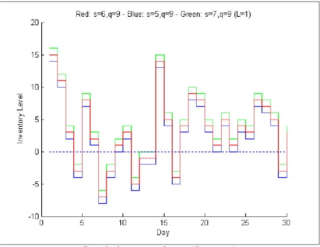
Perturbation Analysis is a technique for gradient estimation from a single simulation. For Perturbation Analysis algorithms, q=S-s will be defined for simplifications.
As can be seen from the graph above, the aim is to find the costs of four neighbors of point (s,q) by only making the simulation for (s,q). Firstly the Perturbation Analysis Algorithm is applied to the parameter s to calculate the delta costs of (s-1,q) and (s+1,q). After that, the delta costs of (s,q+1) and (s,q-1) are calculated by Perturbation Analysis on q parameter. Detailed information about these algorithms can be found below.
3.1 Perturbation Analysis Algorithms 23
3.1.1 Perturbation Analysis on "s" (Algorithm 1)
In this algorithm, the perturbation is done on "s". It means that we leave the S svalue (qvalue) constant and perturbate the system on s to determine the descent direction for the given constant q.
Perturbation on s one by one (Constant q)
Figure that is above shows the effect on sample path where q is xed and s is per-turbed. Red lines denote the On-Hand Inventory when s = 6; q = 9. Green lines denote the On-Hand Inventory when s = 7; q = 9, and blue lines denote the On-Hand Inventory when s = 5; q = 9: It can be easily seen that a perturbation in s shifts the entire sam-ple path by the same perturbation. When s is perturbed by 1 unit, all of the samsam-ple path
3.1 Perturbation Analysis Algorithms 24
is perturbed 1 unit. It means that, when we change s value and keep q value constant, the ordering policy does not change, i.e., we still order the same amount at the same periods. The effect of increasing s is to increase the on hand inventory or to decrease the shortage amount resulting with the change in cost determined by the following algorithm.
Algorithm 1:
The owchart of Algorithm 1 can be found in Appendix A.
3.1.2 Perturbation Analysis on "q" (Algorithm 2)
3.1 Perturbation Analysis Algorithms 25
As seen from the gure above, the perturbation in q may result with a major change on the sample path. Thus, the ordering policies change, i.e. in perturbed path an order may be placed where there was no order in the nominal path.
In the table below, the policy (s = 1; S = 61) is perturbed to become (s = 1; S = 62) for the case of zero Lead Time.
In the table above, the rst row is the demand occured that period. The second row is the Ending Inventory if (s; S) policy is used (Nominal Path). The third row shows the Inventory Position for (s; S) policy. And the last row is the Ending Inventory if (s; S + 1) policy is used (Perturbed Path). To be short, POL1 will be used for (s; S) policy and POL2 will be used for (s; S + 1) policy afterwards. From the table above, we can also see the following points:
Firstly, it is seen that we have to deal with "Delta" values to construct the perturbed sample path. "Delta" value can be de ned as the value in the fourth row minus the value in the second row (how many more units to hold in the perturbed path compared to the nominal path). At the beginning, the perturbed path can be easily calculated as the previous section (only one unit difference between the two paths). However, after some point, the
3.2 Finding Optimal (s*,q*) Pair 26
perturbed path starts to become different from the nominal path. When the path is analyzed carefully, it can be seen that the system starts to get out of order ("delta" values change) after the numbers with red circles in the third row. 61 is the S value of the nominal path. Thus, we can see numerically that the perturbed path gets out of order when Inventory Position reaches the S value. It means that when we reach the S value in POL1, we place an order. However, the S value of POL2 is 62, i.e. we do not place an order in POL2 in the cases where Ending Inventory falls exactly to s in POL1. So, there is an ordering change.
From now on, we focus on the "Delta" values. If POL1 orders and POL2 does not order, we have a "Delta"=-59 for one period and after that period, we have a completely different "Delta" value until we reach another red circle. When we reach the red circle, if both policies order, everything becomes ne, "Delta" again decreases to 1 and continues as 1 until reaching another red circle.
After calculating the perturbed path, things will become similar to Section 3.1.1. We consider the cost differences if we increase or decrease q by 1, and try to solve this optimization problem until we reach the optimal q value for the speci c constant s value.
Algorithm 2:
The owchart of Algorithm 2 can be found in Appendix B.
3.2 Finding Optimal (s*,q*) Pair
For nding the optimal parameters by the perturbation analysis method, the cost graph should be convex. Thus, the cost graph must be convex in s when q is xed, and vice
3.2 Finding Optimal (s*,q*) Pair 27
versa. Sahin (1982) showed that the cost graph is convex in s for xed q values. Thus, the perturbation analysis method can nd the optimal s value by Algorithm 1. However, there are no proofs for Algorithm 2's optimality. When s is xed, there may be some local optimal values such that the perturbation algorithm method can stuck on these values. Since we have different demand sample paths in each period, the local optimal values, if any, change from period to period. Thus, if there are some local optimal values, we can get rid of them while the simulation runs long enough. The convergence to the global optimal value can be satis ed since the global optimal value remains the same in each period.
This chapter will be a combination of Section 3.1.1 and Section 3.1.2. In those sec-tions, how to update one of the control parameters are discussed. In addition to this, by using the methods in the mentioned sections, how to nd the optimal pair will be discussed in this section. s and q values will be updated one by one until the optimal pair is reached. Firstly, we start with an arbitrary (s; q) pair. After that, using Algorithm 1, s value will be updated to s + 1, s or s 1. Then, we have the updated s + 1 value and initial q value. Now, we will perturbate on q value, and update it to q + 1; q or q 1. The process continues on until q and s values do not oscillate.
Algorithm 3:
STEP1: Start with initial s and q values
STEP2: Use Algorithm 1 and update s value (s + 1, s or s 1) STEP3: Use Algorithm 2 and update q value (q + 1; q or q 1)
3.2 Finding Optimal (s*,q*) Pair 28
STEP4: if s and q values were both same at the previous iteration s = sand q = q
else
go back to STEP2.
Example 1 Finding optimal (s; S) pair for the problem below by using Algorithm 3. Demand ~N(5; 2): round the numbers to have integer demands, negative demands are assumed to be zero
Lead Time: 1 day Holding cost/unit: $0.1 Ordering cost: $1 Penalty cost/unit: $30
After starting with initial s = 5 and q = 5, s = 15 and q = 9 (S = 24) is found by running code in Appendix C. The optimal solution could be found in 15 iterations and the gure below shows the iterations from (5,10) to (15,24).
3.3 Initializing Perturbation Analysis Parameters 29
Iterations on s and S
3.3 Initializing Perturbation Analysis Parameters
The Perturbation Analysis will be initialized with values that are the outputs of the Ehrhardt's Heuristic. Thus, the Perturbation Analysis Algorithm will have two main stages:
1. Finding Rough Estimate by using Ehrhardt's Revised Power Approximation 2. Fine Tuning by Perturbation Analysis
As mentioned in Section 2.4, Ehrhardt introduces two heuristics that compute ap-proximation of optimal sE and SE values with simple equations; Power Approximation
3.3 Initializing Perturbation Analysis Parameters 30
optimal values. Both of these heuristics need the knowledge of mean and variance of the demand distribution.
In this thesis, Ehrhardt's Revised Power Approximation will be used without the knowledge of mean and variance. This new heuristic will work as follows; the demand will be observed for some time period. The mean and the variance of this observed demand will be calculated and these calculated values will be used to nd the optimal s and S values. After that period, the policy parameters will be updated and the new mean and variance will be calculated with the new demand data. The MATLAB Code of the Ehrhardt's Heuristic can be found in Appendix D.
The main issue is why to use Ehrhardt's Revised Power Approximation to initial-ize the problem. For running the Perturbation Analysis Algorithm, it is a must to start with some initial values. Ehrhardt's Revised Power Approximation is a very good approx-imation for the optimal parameters. It cannot always nd the optimal but is a really good approximation that only requires some nanoseconds. If the Ehrhardt's Revised Power Ap-proximations is not used, you have to start from an initial point; let's say (10; 30): Then, the Perturbation Analysis will work as the graph below:
3.3 Initializing Perturbation Analysis Parameters 31
However, if the Ehrhardt's Revised Power Approximation were used to initialize the values, the following graph would be obtained:
3.3 Initializing Perturbation Analysis Parameters 32
As can be seen, the PA Algorithm can nd the optimal solution in both cases. How-ever, since the PA Algorithm can update itself one by one, it takes some time to reach the optimal solution in the rst case. Thus, initializing the (s; S) values by Ehrhardt's Revised Power Approximation Method is very advantageous. The graph converges to the optimal value in the 6thperiod. However, after a while, the S value again starts to oscillate because
of different demand sample paths. If the sample path was always the same, after the con-vergence there would be no more oscillations. The converged value would be the optimal value where the Perturbation Analysis method cannot move in either sides for the same demand data.
3.3 Initializing Perturbation Analysis Parameters 33
To conclude, the Perturbation Analysis Algorithm works in the following way: STEP1: Determine a short time period, R (i.e. 7 days)
STEP2: Observe the problem environment for R days
STEP3: Calculate the mean and variance of the demand for the rst R days
STEP4: Use Ehrhardt's Heuristic to calculate the approximate values of sE and SE,
and start with s = sE and q = SE sE
STEP5: Use Algorithm 1 and update s value (s + 1; s or s 1) STEP6: Use Algorithm 2 and update q value (q + 1; q or q 1) STEP7: if s and q values were both same at the previous iteration
s = sand q = q else
34
CHAPTER 4
SIMULATION
4.1 Logical Model
The logical model of the problem can be summarized as the figure below:
As seen from the figure, there are mainly three types of events in our problem; order arrival event at the beginning of the day, demand event during the day, and inventory review event at the end of the day.
Orders arrive at the beginning of the working days. If there is a lead time of zero, the orders arrive in the following morning. On the other hand, the orders will not arrive before the lead time passes. At the beginning of the first day, no orders arrive since no orders were given before. Demands occur during the whole day as integers. Random demands occur in the problem and the distribution of the demands can be any kind of distribution or may have empirical distribution. Thus, during the day, demand D occurs and the ending inventory of the first day becomes "S-D". Inventory position also becomes "S-D".
4.1 Logical Model 35
The inventory is reviewed at the end of every day. At the end of the day, the inventory position is calculated and order is given if the inventory position is below or equal to s. "S Inventory position" units are ordered and waiting orders is updated. Since order is given, the new inventory position will be S. The inventory on hand is also calculated when the shop is closed. Then, we calculate the cost of the rst day from the inventory level. If we have inventory on hand, we will have holding cost at the end of the rst day. On the other hand, if there are unsatis ed demands, there will be penalty cost at the end of the day. Also, an ordering cost will be applied if we have given an order.
The objective of the problem is to choose s and S values such that the summation of the daily costs is minimized.
The general owchart of the problem can be seen in Appendix E.
Numerical Example
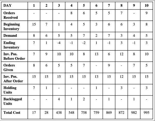
To visualize the problem, a simple numerical example is given below. The example is given for a period of 10 days and the (s; S) values are de ned as (10,15). We have a constant Lead Time of 2 days and demand is uniformly distributed between 1 and 10 units. Demands arrive as integers and the costs are de ned as; holding cost/unit=$1, penalty cost/unit=$100, ordering cost=$10.
As shown from Figure 4.1 and 4.2, at the beginning of day one, the beginning inven-tory is 15. During day one, 8 units are demanded. Since we had inveninven-tory on hand, we have sold all of the 8 items to the customers and at the end of the day we have remaining 7 items on inventory. We order S Y1(15-7=8) items since the "inventory position" is
be-4.1 Logical Model 36 -1 -1 -2 1 4 -Backlogged Units 995 982 872 869 759 758 548 438 28 17 Total Cost DAY 1 2 3 4 5 6 7 8 9 10 Orders Received - - - 8 6 5 5 7 - 9 Beginning Inventory 15 7 1 4 5 3 6 6 3 8 Demand 8 6 5 5 7 2 7 3 4 5 Ending Inventory 7 1 -4 -1 -2 1 -1 3 -1 3 Inv. Pos. Before Order 7 9 10 10 8 13 6 12 8 10 Orders Given 8 6 5 5 7 - 9 - 7 5 Inv. Pos. After Order 15 15 15 15 15 13 15 12 15 15 Holding Units 7 1 - - - 1 - 3 - 3 -1 -1 -2 1 4 -Backlogged Units 995 982 872 869 759 758 548 438 28 17 Total Cost DAY 1 2 3 4 5 6 7 8 9 10 Orders Received - - - 8 6 5 5 7 - 9 Beginning Inventory 15 7 1 4 5 3 6 6 3 8 Demand 8 6 5 5 7 2 7 3 4 5 Ending Inventory 7 1 -4 -1 -2 1 -1 3 -1 3 Inv. Pos. Before Order 7 9 10 10 8 13 6 12 8 10 Orders Given 8 6 5 5 7 - 9 - 7 5 Inv. Pos. After Order 15 15 15 15 15 13 15 12 15 15 Holding Units 7 1 - - - 1 - 3 - 3
Fig. 4.1. Numerical Example of Inventory Simulation for s=10, S=15
low the s value. For the rst day, the cost calculation is done as follows; we have 7 units in inventory, which means a cost of 7x(unit holding cost)=$7. We have no shortages; thus no costs occur from shortages. On the other hand, since we have given an order, an ordering cost (=$10) is also occurred. As can be seen, at the end of rst day, we have a total cost of $17.
After the rst day, the second day starts. We had an inventory of 7 units from the rst day. Also we had ordered 8 items the day before. However, since the leadtime is 2 days, we do not receive any orders this day. At the end of second day, we have a 1 unit inventory on hand, and order 6 items since the "inventory position" is 9 which is less than the "s value".
4.2 Simulation Models 37
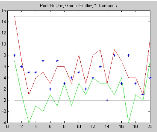
Fig. 4.2. Inventory Simulation Example
Similarly, at the end of the third day, we have 4 backlogged units. From these short-ages, we have a cost of 4x(unit shortage cost)=$400. At the beginning of fourth day, the orders given in rst day are received. And by these manner, the simulation continues. For these 10-days simulation, we have an average cost of $99.5. The algorithms de ned in Chapter 3.1, calculates the optimal s and S values that minimize this average cost by using the method of Perturbation Analysis.
4.2 Simulation Models
4.2 Simulation Models 38
ARENA Model: An ARENA Model was constructed to simulate the problem environment. The distribution of the demand, s; S values, the cost rates, and the lead time are given into the system as the inputs. The outputs are number of holding inventories, number of shortages, number of orders, and the totalcost. The ARENA model can be seen in Appendix F.
EXCEL Model: In the EXCEL Model, the inputs are the same as the ARENA model. However in this model, the outputs can be seen period by period. For example, it can be seen how many units were backordered in 17thperiod, what is the
total cost of 26thperiod, etc. Also the probability of shortage can also be seen in this
model. The EXCEL model can be seen in Appendix G.
MATLAB Model: The MATLAB model works the same way with the EXCEL model. However, it works much faster when compared to the EXCEL Model. Thus, the MATLAB model will be used in the following applications. The MATLAB code that models the simulation can be found in Appendix H.
39
CHAPTER 5
NUMERICAL EXAMPLES
In this chapter, the Perturbation Analysis Algorithm defined in Section 3.3 will be used for different types of demand distributions. The aim of this chapter is to show that the algorithms introduced in this thesis can find the optimal solutions for all different types of demand distributions. In addition to this, the adaptability of the methods will be compared. Adaptability means to find out the new optimal policy parameters after a sudden change in demand.
Three new parameters will be introduced in this chapter; • Delta Day (δ): Period Length (in days)
• Period (Φ): Simulation Length (in periods)
• Demand Period (γ): Moving window's size (in periods)
δ is the time period that a single policy is run. After δ day passes, the (s,S) parameters will be updated and the second Φ starts. As can be understood, Φ is the time period of δ. To give a simple example, lets take δ = 7 days, and Φ = 30. Then, the parameters will be updated in every 7 days, and the total runtime will be 210 days.
γ is the time that is used to compute the new optimal parameters. For example, if we have δ =7 days, γ= 3, the new (s,S) parameters will be calculated by observing the last 21 days' demand history. When γ is larger, iteration number to find the optimal pair will be less. On the other side, when you have very large γ, then the adaptability of the code will be worse. The effects of these parameters will be seen in Section 5.1 and Section 5.3.
5.1 Poisson Distribution 40
In this chapter, rstly, the demand distribution will be taken as Poisson Distribution. In this section, I will compare my results with the results of Zheng&Federgruen (1991) to discuss about the optimal solution. Also, the effects of and values will be discussed in this section.
After that section, the algorithm will be tested with Discrete Uniform and Discretized Normal distributions, respectively. Also, a demand distribution that is created by compo-sition method (Poisson(10) with 40% probability and Poisson(25) with 60% probability) will be taken as the input; and it will be shown that the algorithm can also work with em-pirical distributions. In all of these examples, the Perturbation Analysis Algorithm will be compared to the Retrospective Integer Programming Method and Ehrhardt's Heuristic. Retrospective Integer Programming Method uses the past data and nds the optimal (s; S) pair by using integer programming. This problem is solved in GAMS environment and the GAMS code can be found in Appendix I.
Finally, at the last section of this chapter, the mean of the demand distribution will change suddenly after some time, and the adaptability of the Perturbation Analysis Algo-rithm, Retrospective Integer Programming Method and Ehrhardt's Heuristic will be com-pared for different and values.
5.1 Poisson Distribution
In this section, Poisson Distribution with mean 10, and with mean 25 will be taken as the demand distributions. Zheng&Federgruen (1991) studied about the Poisson Distribution and founded the following results:
5.1 Poisson Distribution 41
s S c 10 6 40 35:022 25 19 56 54:262
The table shows that, for Poisson(10), the optimal solution is found as (6; 40) with an average cost of 35:022. When the mean is 25, the optimal solution becomes (19; 56) with an average cost of 54:262: The costs are taken as; holding cost rate h = 1, penalty cost rate p = 9, and xed setup cost K = 64 with no leadtime (L = 0). In this section, to compare the Perturbation Analysis Algorithm with the algorithm de ned in Zheng&Federgruen (1991), in all of the examples the input parameters will be taken as given above (h = 1; p = 9; K = 64; L = 0).
5.1.1 Poisson Distribution (10) with No Lead Time
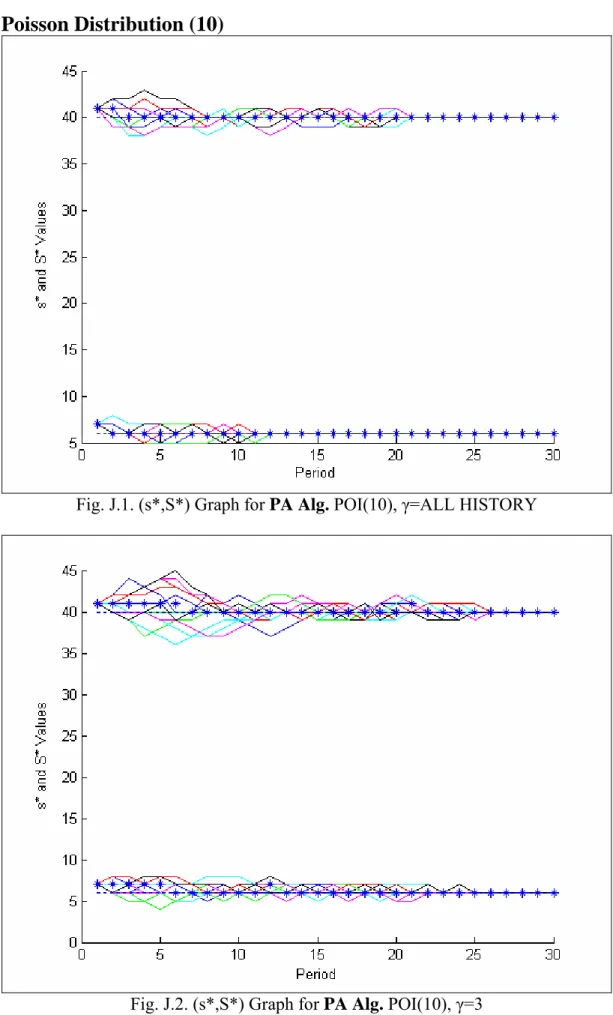
The optimal (s; S) parameters are found as (6; 40) in Zheng&Federgruen (1991) for the input parameters de ned above. As de ned in Section 3.3, the Perturbation Analysis Al-gorithm initializes the s and S values with the Ehrhardt's AlAl-gorithm. While the Ehrhardt's Heuristic is run for the rst Period, sE = 7; SE = 41is found. Thus, the algorithm starts
with s(1) = 7; S(1) = 41: Then, different sample paths are generated for each runs. The output of Perturbation Analysis Algorithm for 20 runs can be seen in Fig.J.1-Fig.J.2 in Appendix J.
For = 3; when we look at the graphs Fig.J.2, Fig.J.4, Fig.J.6, it is seen that the optimal values oscillate a lot, and in the periods, the algorithms nd different optimal values in different runs. When we look at the ensemble average graph (Fig.J.8), it is seen that the average values in Perturbation Analysis Algorithm converges to the optimal values. There
5.1 Poisson Distribution 42
is a dispersity because of the small value. It means that the algorithms only take the previous 3 Periods' history and it cannot be enough to nd the exact optimal values. When the algorithms' cost are compared (Fig.J.10), it can be seen that the Perturbation Analysis Algorithm has the smallest cost where the Ehrhardt's Heuristic has the largest cost.
When the value is increased, the optimal (s; S) values start to oscillate near the optimal values in Perturbation Analysis Algorithm (Fig.J.1). All of the runs give the same optimal (s; S) values after some time. The Retrospective Integer Programming Method and the Ehrhardt's Heuristic also converge to some value, but they are not the optimal values (Fig.J.3, Fig.J.5). Ehrhardt's Heuristic overestimates the (s; S) values where the Retrospective Integer Programming Method usually underestimates. When looked at the cost functions, Fig.J.9, as in the rst part Perturbation Analysis Algorithm gives the least cost where Ehrhardt's Heuristic gives the most.
5.1.2 Poisson Distribution (25) with No Lead Time
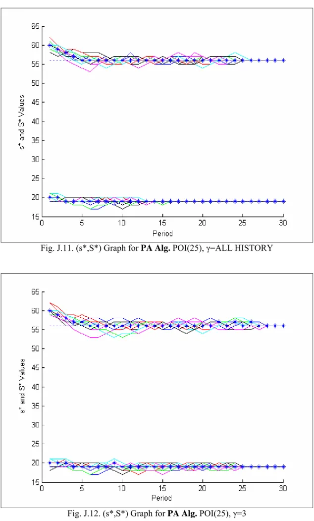
This part is another example for the Poisson distribution. In Zheng&Federgruen (1991), the optimal solution is calculated as (19; 56) and by the Perturbation Analysis Algorithm, the graphs (Fig.J.11, Fig.J.12) in Appendix J are obtained after 20 runs.
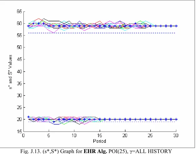
The analysis made in Subsection 5.1.1 are also correct for this subsection. When the value is small, the optimal solutions of the algorithms oscillate a lot. However, the ensemble average of the Perturbation Analysis Algorithm converges to the optimal values (Fig.J.18). When this value is increased, the algorithms start to get better results. In ad-dition to this, Ehrhardt's Heuristic again overestimates the policy parameters and can only
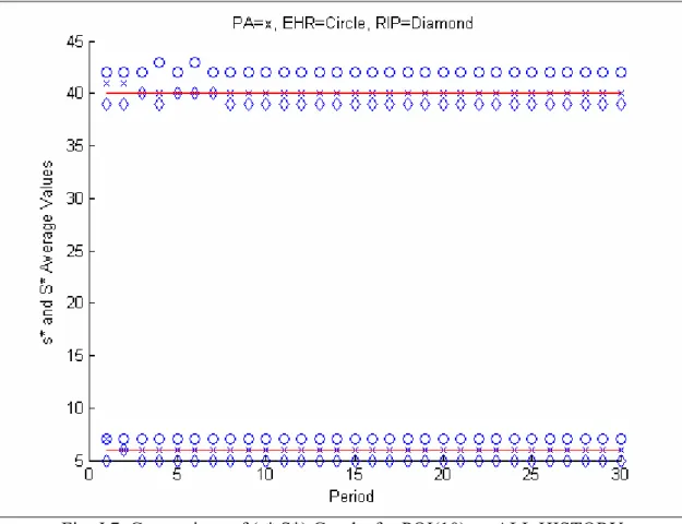
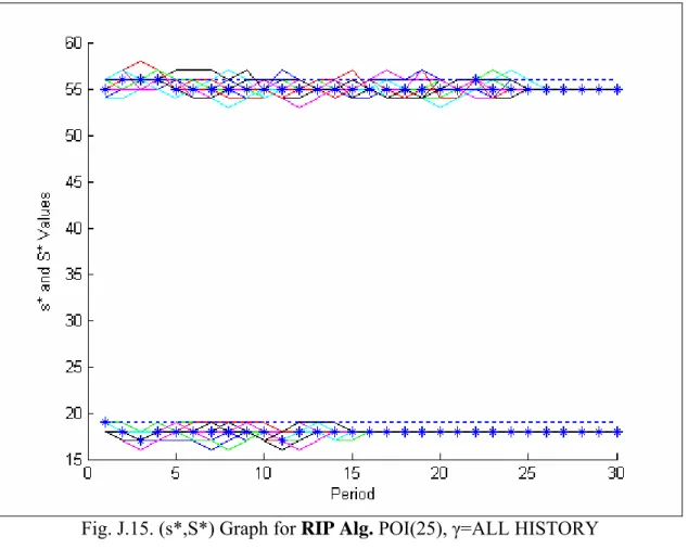
5.1 Poisson Distribution 43
nd values that are near optimal, not optimal. (Fig.J.13 - Fig.J.14) The Retrospective Inte-ger Programming Method usually underestimates the policy parameters (Fig.J.15, Fig.J.16) and the Perturbation Analysis Algorithm, again, has the minimum cost (Fig.J.19, Fig.J.20). Zheng&Federgruen analyze 24 examples in their paper. I had also run all of these examples with the Perturbation Analysis Algorithm, Ehrhardt's Heuristic, and Retrospec-tive Integer Programming Method, and found the following results (these results are the averages of 20 runs for each example):
In the table above, the green color represents optimal values, yellow values represent the values that are above optimal and the red color represents the values that are below the optimal. It is easy to see that the Perturbation Analysis Algorithm can nd the same
op-5.2 Comparison with Other Algorithms 44
timal solutions as Zheng&Federgruen's Algorithm for all of the 24 examples. Ehrhardt's Heuristic always overestimates the policy parameters and Retrospective Integer Program-ming Method usually underestimates.
5.2 Comparison with Other Algorithms
In this section, several demand distributions will be compared by other algorithms; i.e. Ehrhardt's Heuristic and Retrospective Integer Programming Method. The aim is to check whether the algorithms can nd the optimal solutions for these distributions.
5.2.1 Uniform Distribution (0,10) with Lead Time=1 Day
In this section, Discrete Uniform Distribution with minimum value of 0, and maximum value of 10 is taken as the demand distribution.
By running the algorithms presented in this thesis, the following results are obtained: After running the code which is in Appendix H, the optimal s and S values are found as 15 and 24 in a time of 40.12 seconds. It means that when all of the (s; S) pairs' cost is calculated, the minimum cost will be satis ed with the (15; 24) pair.
For this distribution, as seen from Fig.J.21-Fig.J.22 Perturbation Analysis Algorithm again converges to the optimal parameters and has the minimum cost when compared to the other two methods.
5.2 Comparison with Other Algorithms 45
5.2.2 Normal Distribution (5,1) with Lead Time=1 Day
In this section, Normal Distribution is taken as the demand distribution with the parameters of Mean=5, Std.Dev=1. Since normal distribution is a continuous distribution, the values had been rounded to the nearest integer to have integer valued demands, and the negative demands will be taken as no-demand.
By running the algorithms presented in this thesis, the following results are obtained: After running the code which is in Appendix H, the optimal s and S values are found as 11 and 18. It means that when all of the (s; S) pairs' cost is calculated, the minimum cost will be satis ed with the (11; 18) pair.
Again for the Normal Distribution, the Perturbation Analysis Algorithm converges to the optimal parameters and has the minimum cost when compared to the other two methods. The gures (Fig.J.23-Fig.J.24) can be seen in Appendix J.
5.2.3 Empirical Distribution
In this section, the demand distribution does not have a speci c distribution. This distri-bution is a combination of Poisson(10) and Poisson(25) distridistri-butions with 40% and 60% probabilities, respectively where the demand distribution is created by the Composition Method. In this case, all of the three algorithms can work well since all of them use the previous data, without the knowledge of variance and mean. The optimal values of the (s; S)parameters are found by the code in Appendix H and the optimal (s ; S ) values are found as (14; 49): Perturbation Analysis Algorithm has the minimum cost when compared
5.3 Adaptability 46
by the other two methods. The graphs about this section (Fig.J.25-Fig.J.26) can be seen in Appendix J.
5.3 Adaptability
For the adaptability issue, in the rst 20 periods the demand distribution is taken as POI(10). After the 21st period, the demand distribution changes to POI(25). In this section, the aim
is to check if the methods can adapt themselves to the sudden demand changes.
5.3.1
= 15
Days,
= 3
Periods
When value is very small, from Fig.J.27-30, it is seen that all of the methods (Perturbation Analysis Algorithm, Retrospective Integer Programming Method and Ehrhardt's Heuristic) are all adaptive for sudden changes. When we analyze the rate of adaptability, it is seen that the Perturbation Analysis Algorithm cannot adapt itself as quick as the other methods. It is an expected result since the Perturbation Analysis Algorithm can update itself one by one. The Retrospective Integer Programming Method and Ehrhardt's Heuristic update themselves very quickly since they only consider the last three periods' demand data. On the other hand, all of the algorithms cannot converge to a single value quickly. It means that when the value is very small, the methods cannot converge to the optimal value quickly but the adaptability for sudden demand changes is quite good.
When the ensemble averages of the 20 runs are considered (Fig.J.30), it is seen that the average optimal values of Perturbation Analysis Algorithm converge to the real optimal
5.3 Adaptability 47
values. On the other hand, Ehrhardt's Heuristic overestimates and Retrospective Integer Programming Method underestimates the optimal values as also discussed in Section 5.1.
5.3.2
= 15
Days,
=
All History
When we keep the same but only increase the value, it is seen that convergence rate decreases (Fig.J.31-34).
For the Perturbation Analysis Algorithm, the S value starts to converge around a value in 35th period where it was 33rd period in Section 5.3.1. The s value also starts to
converge around a value in 39thperiod where it was 35thperiod in the previous section.
The change of the convergence rate can be seen better in Ehrhardt's Heuristic. That method could converge in ve periods when was very small. However, when it is in-creased, it needs about ten periods to converge to the new values.
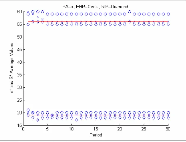
On the other hand, the values oscillate in speci c values instead of a big range of values when the value is increased. When looked at Fig.J.28, the S value in Perturbation Analysis Algorithm converges to values between 54-58 when value was small. However in Fig.J.32, the algorithm converges to only three values; 55, 56, 57.
The ensemble average graph is very similar to the previous section. Perturbation Analysis Algorithm can converge to the real optimal value where Ehrhardt's Heuristic over-estimates and Retrospective Integer Programming Method underestimate.
5.3 Adaptability 48
5.3.3
= 90
Days,
=
All History
In this section, the effect of will be analyzed. From Fig.J.35-38, it is seen that when the value increases, convergence to a single value can be satis ed earlier since much more days' demands are observed. After observing 90 days' demand, the (s; S) values are updated and it helps to converge to a speci c value. The disadvantage of increasing cannot be seen from the graph. However, when the is taken as a big value, then the s, S values cannot be updated for a large number of days and it decreases the exibility of the inventory policy since the period time increases.
49
CHAPTER 6
CONCLUSIONS AND FUTURE
DIRECTIONS
Inventory policies are used to determine when and how many units to order. For the periodic review policies, the most common inventory policy is the (R,s,S) policy. In this policy, it is known that if the parameters of the system are chosen appropriate, there is always an optimal solution, i.e. the expected period cost can be minimized.
For finding the optimal policy parameters, if the demand distribution is known, exact methods and heuristics are used in the literacy. In this thesis, it is assumed that the demand distribution is not known. The mean and the variance of the demand distribution are also not known. For this case, a perturbation analysis based method is introduced. This method (Perturbation Analysis Algorithm) initializes itself from a heuristic named Ehrhardt's Revised Power Approximation. After the initialization, the method anticipates the sensitivity of (s,S) parameters to the period cost and updates itself to find the optimal (s*,S*) pair.
The outputs of Perturbation Analysis Algorithm were firstly compared with the results of Zheng&Federgruen (1991) for the Poisson Distribution. In all of the twenty-four examples, the Perturbation Analysis Algorithm could find the same optimal values. After that, the Perturbation Analysis Algorithm was compared by two other methods, Ehrhardt's Heuristic and Retrospective Integer Programming Method for several demand distributions, including the empirical distribution for twenty runs. In all of the examples, the Perturbation Analysis Algorithm could oscillate on the optimal solution.