SUMMARY
Making use of the propensity score matching method, we match earlier crises (pre-2007) with currently ongoing crises (post-(pre-2007). The old and new crises are matched in three dimensions: the global setting in which they occurred, the struc-ture of the economy and the domestic vulnerabilities in the pre-crisis period. Our findings suggest that the euro periphery crises share sufficient commonalities with earlier crises in their pre-crisis domestic vulnerabilities. The study points to two important conclusions. First, the euro periphery crises are composed of unique country experiences; hence, it will not be easily resolved with a ‘one-size-fits-all’ set of economic policies. Secondly, while each banking crisis has its inherent uniqueness, each crisis also shares sufficient commonalities with one or more of the Asian-5 1996/97 crises, the Nordic banking crisis of the early 1990s or the Japanese banking crisis of the 1990s. Thus, the extensive knowledge accumulated through these former banking crises can help in designing recovery policies.
—
— Selin Sayek and Fatma Taskin
Financial
crises
Economic Policy July 2014 Printed in Great Britain © CEPR, CES, MSH, 2014.
Financial crises: lessons from
history for today
Selin Sayek and Fatma Taskin
Bilkent University1. INTRODUCTION
Financial crises are not new. Countries all over the world have experienced economic crises for a very long period of time. However, the latest of these crises that started off as a credit crisis in the US and spread to Europe very rapidly, has distinctive charac-teristics. First and foremost, the origin of this crisis that evolved from a pure credit cri-sis into one of an intertwined banking and sovereign debt cricri-sis in Europe within a couple of years (what is now labelled as the euro crisis) is on account of a global shock.1 Crises such as the 2008–2009 financial crisis where ten or more advanced countries synchronously experience a crisis are labelled as synchronous crisis.2
The authors would like to thank the Managing Editors, the anonymous referees, Domenico Giannone and Karl Whelan as well as the panel participants for their very valuable and significant contributions to the analysis.
The Managing Editor in charge of this paper was Philip Lane.
1
In the remainder of the paper the Euro crisis will refer mainly to the crisis of the periphery eurozone countries, namely Greece, Ireland, Italy, Portugal and Spain (GIIPS).
2
According to the April 2009 World Economic Outlook, 1975, 1980, 1992 and 2008–2009 are the four episodes that are labelled as synchronous crisis periods.
Economic Policy July 2014 pp. 447–493 Printed in Great Britain © CEPR, CES, MSH, 2014.
Second, the euro crisis is experienced by the sui generis European Monetary Union, a union that has no historical precedent.3
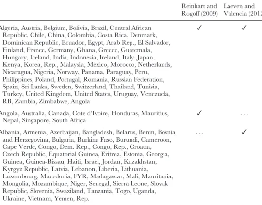
Despite its distinctive characteristics, on the other hand, the euro crisis shares two main features with the remaining recent financial crises: problematic public debt levels as well as a fragile banking system. The latter of these has indeed led the euro crisis to be labelled as a banking crisis by the two most comprehensive crisis datasets (Reinhart and Rogoff, 2009; Laeven and Valencia, 2012). Both datasets identify the GIIPS countries as experiencing a banking crisis starting in 2007 or 2008.4The same datasets include many more country experiences that are labelled as banking crisis: a total of 117 countries are identified as experiencing 165 separate banking crisis episodes during 1980–2011. This statistic begets the question of whether the ongoing GIIPS crisis shares commonalities with any of these past banking crises. This paper sets out to test this question and identify if the domestic vulnerabilities of the GIIPS economies prior to the 2007/2008 global financial crisis bear sufficient similarities with any past crisis experiences.
The analysis also addresses whether the individual country crises in the euro periphery are different from each other or whether there is a single euro crisis. The answer to this question would not only satisfy one’s intellectual curiosity of whether the sui generis European project has led to a sui generis set of financial crises but would also provide a framework for policy discussions.
Accordingly, we will provide information on within-variation in the GIIPS group of countries, as well as the variation between the GIIPS group and the rest of the world. The evidence regarding the within-GIIPS variation, that is, the test of whether individual periphery European crises are sufficiently different from each other, will allow discussing whether one-size fits all policies or individual country-customized policies should be designed. The evidence regarding the variation between the ongoing and past crisis experiences, on the other hand, would allow the policy design discussions to benefit significantly from the vast information available from these past experiences.
These questions are not novel. In fact, there is a large literature on whether or not this set of crises is different. What is novel in this paper, however, is the method used in providing evidence for these questions. The existing literature that analyses this question seeks the answer to whether on average the nature of crises change over time and/or across countries. These studies tend to base their analysis on the early warning
3
The terminology comes from Eichengreen (2008).
4 According to Reinhart and Rogoff (2009) Greece, Ireland and Spain experienced both a banking and a
stock market crisis at the outset of the global financial crisis, whereas Italy experienced a stock market cri-sis and Spain experienced a banking cricri-sis. Laeven and Valencia (2012) identifies Italy and Portugal as experiencing extensive liquidity support and significant liability guarantees, and as such borderline sys-temic banking crises; while Greece and Spain also experiencing significant restructuring costs, and Ireland furthermore experiencing significant asset purchases and nationalization beyond what Greece and Spain experienced.
systems (EWS) framework to predict crises.5The major goal of the EWS framework is to develop a set of stable variables that will signal a crisis before it actually occurs and will assist in avoiding very costly banking crisis outcomes. The underlying assumption of the EWS framework is that new crises provide new information that can be com-bined with previous information provided by old crises since crisis across different time periods have similar properties. If, however, the EWS analysis does not point to such a stable set of variables then this result is indicative of the changing nature of crises. Studies by Gupta et al. (2007), Rose and Spiegel (2010, 2011), Frankel and Saravelos (2012) among several others test for such differences making use of the EWS framework. The purpose of these analyses is to explore whether or not these crises are different from each other on average. For example, an EWS framework seeking evidence for whether the crises between the Latin American region (or the 1980s) and the East Asia and Pacific region (or the 1990s) are different would provide information on whether, on average, the probability of going into a crisis is different for Latin America (or the 1980s) or East Asia and Pacific (or the 1990s). However, the outcome could hold possible divergences from such average behaviour. While the average behaviour might differ significantly between regions or across time, it could easily be that an individual country experiences something similar to what an individual country in a different group experiences.
In fact, the discussion of whether a crisis is different than past experiences is one that flares up at the onset of each crisis. Following the late 1990s in respect of emerging mar-ket crises, for example, a controversial debate arose of whether the crises were geograph-ically more widespread, were deeper, or whether models based on past crises at the time could have predicted the occurrence of these. In this debate, for example, Eichengreen and Rose (1998) and Berg and Patillo (1999) argued that although past experiences pro-vided some information on the new crises, the predictive power of such general models was limited. They reasoned that this limitation was a reflection of the differences in crises experiences across time and/or across countries. Kaminsky and Reinhart (1998), on the other hand, argued that the existing regional differences between East Asia and Latin America eroded strongly during the 1990s, rendering their crises similar. This is echoed in the findings of Kamin (1999) as well. He argued that exchange rate behavi-our, the fall in output, current account adjustments and financial sector difficulties were very similar to past episodes of crises despite the larger incidence of emerging market crises at the time. Edison (2003) studied the differences across regions, making use of an early warning system (EWS) framework. The findings lent support to the premise that there were no significant statistical differences across regions.
The start of the ongoing crisis also spurred similar discussions, for which Claessens et al. (2010, 2013) provide an overview. Rose and Spiegel (2010, 2011) consider a
5
Such studies have once again come centre stage, with important contributions from Reinhart and Rogoff (2009), Rose and Spiegel (2010, 2011, 2012) and Frankel and Saravelos (2012), among many others.
purely cross-sectional analysis to examine the link between the occurrence and severity of crises, drawing on macroeconomic and financial indicators that have been previously identified as relevant indicators for crisis prediction. Their goal is to mainly study whether the crisis incidence differs across regions, rather than focusing on across time differences. They interpret the lack of robust findings as suggestive of crisis experiences differing across regions. By extending the dataset further into the ongoing crisis, Frankel and Saravelos (2012) also conducted an exercise of identifying the relevant variables in explaining the 2008–2009 crisis incidence. With some reserva-tions, they argue that, despite the differences in financial crisis characteristics across years and regions, their empirical investigation of the 2008–2009 crisis lends support to using early warning indicators to explain crisis incidences and provide supportive evidence to the hypothesis that the nature of crises do not change significantly tempo-rally or regionally.
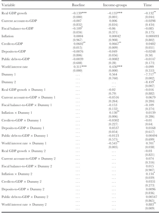
Our goal is not to contribute to this literature on predicting banking crises. Rather, we would like to make use of this framework to roughly test whether the factors that contribute to predicting the crisis have changed across time or across countries. This is done rather as a prelude to our main analysis that allows speaking beyond averages and going into the crisis specificities. The results of this prelude exercise are presented in Appendix 1, where we report the results from logit regressions that we run in line with the EWS framework by including dummy variables that capture the fact that the ongoing GIIPS crisis is one of high-income countries and has occurred temporally recently. Results point to the governing factors showing ample similarities across country groups, as well as across time. The role of real GDP growth, the current account dynamics, the fiscal balance, private sector credit and public debt in contributing to the probability of a crisis occurring remains unchanged across lower and high-income countries, as well as across time periods. However, alongside these similarities, there seems to be some differences. The role played by inflation and the world interest is found to be different across income groups and across time. These results are suggestive of the fact that the current ongoing high-income country bank-ing crises bear, on average, both commonalities and differences with past and lower-income-country banking crises.
While this framework allows comparison of crises on average, it does not allow identifying case-specific information. The information of whether crises are different from each other on average hides possible divergences from average. In order to identify such case-specific information, a tool that would not purely rely on the infor-mation regarding the relationship between averages but would also take into account individual specific information is preferable. One such tool is the matching tech-nique. The matching technique aims to statistically match/pair similar observations. As such, it is nothing but a way of clustering observations according to a set of pre-determined dimensions. The clusters are pre-determined based on a metric that is obtained within the matching exercise. Indeed the novelty of this paper is to study the aforementioned commonly asked questions using the matching technique by
allowing for identification of similarities of the individual euro periphery crises, both among themselves as well as with earlier historical crises.
In other words, in this paper we test for how the individual country experiences diverge from the average in the build-up towards a banking crisis, and seek to identify which past banking crisis experiences (if any at all) share commonalities with the indi-vidual euro periphery crises. To do this, we choose the propensity score matching technique, which makes use of the pre-crisis conditions and, rather than focusing on averages, is guided by individual specific information.
Our empirical results show that the GIIPS crisis is significantly different than past banking crisis experiences in terms of the structure of the economies experiencing a crisis and in the global conditions during which their respective crises occur. However, the results furthermore show that albeit these differences, the GIIPS economies share extensive commonalities in their domestic vulnerabilities– in their respective pre-crisis periods– with several past banking crisis experiences.
An interesting and important finding is that the GIIPS crisis encompasses some very dissimilar crises as well as very similar ones. For example, the Spanish and Irish crises share a significant amount of similarities in their pre-crisis conditions whereas the Greek crisis is very distinct from all other GIIPS crises. This finding per se is the first evidence against a one-size-fits-all policy prescription for the GIIPS countries. Therefore, the policy design of each country’s recovery should take into account the particularities of each crisis.
The results regarding the matches of the current euro country crises and past crises also present crucial information about the nature of the ongoing crises and their build-up period. The euro periphery crises match mainly with the banking crises of the 1990s. Namely, the experiences of several of the big-five crises (Japan, 1992; Norway, 1987; Finland, 1991) and the East Asian crises (Thailand, 1997; Malaysia, 1997; the Philippines, 1997; Indonesia, 1997) are very important sources of informa-tion regarding the development/evoluinforma-tion of the ongoing crises in Europe.6 These individual matches also allow for a discussion of policy guidelines that are custom made, and the advantage of using the matching technique becomes very clear when discussing the policy prescriptions for the GIIPS.
The evidence provided in the following analysis underlines the different policy priorities for each GIIPS country. Results point to the need for Italy, Spain and Ireland to concentrate on banking sector restructuring and regulation, whereas for Portugal and Greece to concentrate their efforts in designing policies that will allow for a real exchange rate devaluation through a series of policies that will lead to competitive disinflation if not with a radical choice of a nominal exchange rate
6
The ‘big-five’ crises include the Japanese banking crisis (1992), the Scandinavian banking crises (Finland, 1991; Sweden, 1991; and Norway, 1987) and the Spanish crisis (1977).
devaluation. Another important finding concerns the role played by the fiscal sustain-ability position of each country in leading to differential fiscal policy advice.
The rest of the paper is organized as follows: data are defined in Section 2, the methodology and results are presented in Section 3, and Section 4 concludes.
2. DATA
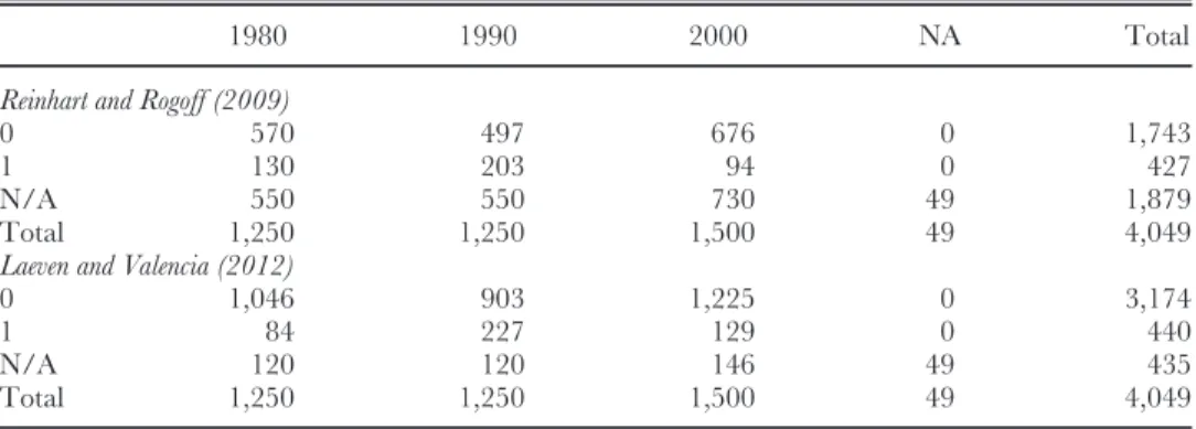
In order to discuss similarities across the current and previous banking crises, it is necessary to identify the dates of the crises. In doing so, we rely on existing studies in the literature, which specifically identify the banking crises through assessment of qualitative events.7These are two of the most recent updates of such datasets by Rein-hart and Rogoff (2009) and Laeven and Valencia (2012), who base their crisis dates on the pioneering work of Caprio and Klingebiel (2003) and Demirg€ucß-Kunt and Detragiache (1998, 2005).
We reconstructed a banking crisis indicator identifying a year as a crisis year pro-vided either Reinhart and Rogoff (2009) or Laeven and Valencia (2012) reports that year as a crisis year. In other words, given the qualitative nature of the construction of these two data series, the judgments made by these two groups of researchers were equally weighted. If either one of them interprets events in a country as being suggest-ive of a banking crisis, we took that as signalling sufficient trouble to be labelled as a crisis. In doing this, no loss of information is incurred, given the already ad hoc nature in identifying the start and end year of a banking crisis in the literature.8 This approach is similar to that used by Gupta et al. (2007) in classifying a currency crisis and Hutchison and McDill (1999) in classifying a banking crisis. Given that our reference includes only two studies, we view it as being significant if even one of them identifies a year as being a banking crisis year.
Reinhart and Rogoff (2008a, 2008b and 2009) see a banking crisis as the occur-rence of either one of the following events: first, if the operation of a bank leads to the closure, merging or takeover by the public sector of one or more financial insti-tutions; and, second, if there are no bank runs but closure, merging, takeover, or large-scale government assistance of an important financial institution takes place. This definition leads to the inclusion of both systemic and non-systemic banking cri-ses in the dataset.
Laeven and Valencia (2012), on the other hand, only include systemic banking crises in their dataset. Systemic banking crises are defined as periods of significant
7
There are also papers that assess banking crises using information on the evolution of financial condi-tions that include large changes in asset prices and/or credit volumes. For example, Gourinchas et al. (2001) identify crises based on deviations of credit to GDP ratio from its trend; Mendoza and Terrones (2008) identify them as large deviations of real credit growth from its trend; Claessens et al. (2010), on the other hand, refer to the peaks and troughs of the level of real asset prices and credit in identifying crises.
8
For more details please refer to Reinhart and Rogoff (2009) and Laeven and Valencia (2012) who raise their respective concerns about the difficulty of knowing exactly when a crisis starts and when it ends.
signs of financial distress in the banking system, and periods during which there are significant banking policy intervention measures to counteract significant losses in the banking system. Such policy interventions are viewed as significant if they include at least three of the following policies: extensive liquidity support, high bank restructuring costs, significant bank nationalizations, additional guaran-tees put in place, significant asset purchases, deposit freezes and/or bank holidays.
The list of countries having experienced a banking crisis according to this reconstruction and the information according to which original dataset the crisis iden-tification is based on, is provided in Appendix 2. This section also provides summary comparisons across the Reinhart and Rogoff (2008a, 2008b) and Laeven and Valencia (2012) datasets.
Table 1 provides an overview of these crises years and episodes, depicting informa-tion over time in panel (a), across regions in panel (b) and across different income groups in panel (c). The sample includes 637 crisis years for a total of 117 countries during 1980–2011. These 637 crisis years correspond to 165 episodes of crisis. A total of 132 of the 165 banking crisis episodes used in this paper took place in the 1980s and 1990s. Of the remaining crises, 25 started in 2007/2008 and are still ongoing. Hence, making use of the information provided by the past 140 crises to shed light on the ongoing 25 crises is a very valuable exercise.
The crises that took place in the 1990s are shorter on average than crises that took place in the 1980s. The majority of the crisis episodes took place in sub-Sah-aran Africa and Europe, followed by Latin America and the Caribbean. The cri-ses in the East Asia and Pacific region, though a less frequent event in terms of counts of crisis episodes, are much lengthier than crises in other regions. The dis-tribution of these banking crisis episodes across the different income groups of countries is very similar, with around 58% of the crises taking place in upper mid-dle or high-income countries and the remainder taking place in lower-midmid-dle and low-income countries.
The data sources and definitions of the variables included in the analysis are given in detail in Appendix 2. While the dataset includes 165 banking crisis episodes, given the non-systematic availability of several macroeconomic variables included in the analysis, the effective sample is smaller.9The variables of interest are annual.
Table 2 shows the evolution of the explanatory variables during times of tranquil-lity, defined as no crisis years as opposed to crisis times. The simple means tests sug-gest that the growth and inflation performance of economies, as well as the fiscal balance and credit extensions as a share of economic activity, differ significantly between tranquil periods and banking crisis periods.
9
This is a problem that affects the whole of this literature on financial crisis. See Gupta et al. (2007), Rose and Spiegel (2010, 2012).
3. METHODOLOGY AND MATCHES
Our ultimate goal is to provide an alternative anatomy of the ongoing European financial crisis in light of this globally accumulated banking crisis experience. In order to make use of this vast experience of past crises, it is essential to search for evidence regarding the similarities and/or commonalities across the current and past crises. In other words, if indeed the euro periphery crises are not different than past experiences then, knowing with which past crises the current crises share a significant amount of commonalities would provide very valuable information. The summary statistics pre-sented in Table 1 suggest that banking crises are phenomena that are not restricted to a certain time period, a certain geographic region or a set of countries. As Reinhart
Table 1. Summary statistics of crisis years and episodes
Panel A. Over time
Decades Tranquil Crisis N/A Total
Average length of crisis No. of episodes 1980–89 893 160 9 1,062 4.06 52 1990–99 844 326 10 1,180 3.80 80 2000–12 1,242 151 23 1,416 3.61 33* Total 2,979 637 42 3,658 . . .
Panel B. Over regions
Geographic Region Tranquil Crisis N/A Total
Average length of crisis
No. of episodes
Americas 45 16 1 62 5.33 3
East Asia and Pacific 230 78 33 341 5.07 15
Europe 629 146 0 775 3.84 38
Europe and Central Asia 430 66 0 496 2.87 23
Latin America and the Caribbean 428 129 1 558 3.88 33
Middle East and North Africa 216 31 1 248 3.88 8
Oceania 26 4 1 31 4.00 1
South Asia 110 13 1 124 3.25 4
Sub-Saharan Africa 865 154 4 1,023 3.85 40
Total 2,979 637 42 3,658 . . .
Panel C. Over income groups
Region by income Tranquil Crisis N/A Total
Average length of crisis No. of episodes High-income countries 829 190 35 1054 4.02 47 Upper-middle-income countries 802 187 3 992 3.90 48 Lower-middle-income countries 746 151 2 899 3.47 43 Low-income countries 602 109 2 713 4.04 27 Total 2,979 637 42 3,658 . . .
Notes: Own calculations from the merging of datasets of Reinhart and Rogoff (2009) and Laeven and Valencia (2012).
The income classification follows the World Bank’s classification, whereas the geographic regional classification follows that of the UN.
and Rogoff (2008a, 2008b) emphasize, these statistics are evidence that the incidence of banking crises in high-income countries is no different from that of middle- or lower-income countries. In our sample, the number of banking crisis episodes in Europe is only two fewer than those in sub-Saharan Africa. The information summarized in this table lends support to justifying a more detailed statistical analysis of whether indeed the nature of banking crises are similar across time and across country groups.
More specifically, we seek to identify whether the GIIPS crisis experiences that are predominantly part of a synchronous crisis period (or a global crisis) and occur in a peculiar set of economies that are structurally different than non-industrial economies, are similar in any way in their domestic vulnerabilities with these very different eco-nomically structured economies in their own crisis experiences. In other words, we are interested in identifying the similarities/discrepancies of the recent crises and the older crises in three dimensions: the global environment during which they occurred; the structure of their respective economies; and the domestic vulnerabilities that are known to lead to financial crisis. One such method of identifying these similarities is propensity score matching.
Our goal is to find similarities or discrepancies of two different sets of coun-tries in these three dimensions. In essence, this exercise is very similar to the
Table 2. Comparison of macroeconomic conditions between tranquil and banking crisis periods
Variable name Tranquil Crisis
Difference of means t-test (p-value)
Current account-to-GDP Mean –3.49 –3.25 –0.565 (0.57)
Median –2.88 –2.40
No. of obs. 2506 575
Fiscal balance-to-GDP Mean –2.20 –3.94 5.760 (0.00)
Median –2.35 –3.70 No. of obs. 1848 360 M2/NFA Mean 32.62 16.17 1.070 (0.29) Median 3.27 3.87 No. of obs. 2371 542 Inflation Mean 27.96 143.24 –4.516 (0.00) Median 5.75 8.88 No. of obs. 2451 566
Private sector credit-to-GDP Mean 42.90 56.22 –6.384 (0.00)
Median 27.33 34.45
No. of obs. 2327 528
Public debt-to-GDP Mean 65.51 76.73 –3.840 (0.00)
Median 53.60 59.15
No. of obs. 2577 596
Bank deposits-to-GDP Mean 40.47 45.59 –2.660 (0.01)
Median 30.20 31.86
No. of obs. 2314 535
Real GDP growth rate Mean 3.83 1.37 8.981 (0.00)
Median 3.94 2.14
matching exercises conducted in the programme evaluation literature. Propensity score matching is a statistical matching technique that allows for matching the entities that received a treatment, or were exposed to a policy/programme with those that have not. Unlike the programme evaluations our emphasis will be on the first stage of the exercise that determines matches between a ‘treated’ and a ‘control’ group. The propensity score is the probability that the entity in question will be treated on the basis of that entity’s characteristics (covariates). Intuitively, the propensity score is a measure of the likelihood that an entity would have been included in the ‘treated’ group given its background character-istics (covariates).
In this propensity score matching exercise, we define the treated units as the crisis episodes that occur on or after 2007 and the control group as all the crisis episodes that occur prior to 2007. We label the treated group as ‘new’ crises and the control group as the ‘old’ crises. Conditional on whether a country has been in a crisis at some point, we match the new crisis with the old crisis. As such, the dataset used to carry out the matching exercise includes the 165 episodes of crisis (non-crisis episodes are not included in the dataset), where the dichotomous variable 1/0 reflects the new/old crises. This exercise interprets ‘being in a crisis currently’ as a treatment, where treat-ment is per se nonsensical, but the exercise helps answer the question of whether the crises in the two periods can be matched sufficiently reliably, and if so, which country pairs match.
In order to carry out this matching exercise we first have to estimate the propensity scores, then implement a matching technique to observe the similarities of current and past economic crises. The propensity score is estimated by logistic regression where the treatment variable (in our case the dichotomous new/old crisis indicator) is the outcome and the covariates are the predictor variables in the model. It is important to note that the propensity score estimated is not an estimation of the prob-ability of a crisis occurring. Rather it is the estimation of whether, given its character-istics, any of the old crises look like any of the new crises. In short, the propensity score is solely a metric that shows the economic distance between the different banking crises. If this distance is small between an old and new crisis this suggests that these two crises share sufficient commonalities in the predictor variables in question.
One important step in this exercise is to determine the variables that will be used in estimating the propensity scores. The three dimensions in which we are interested in identifying the distance between the recent and older crisis are: first, the global condi-tions in which the crisis occurs; second, the structure of the economy in crisis; and, third, the domestic vulnerabilities of the country prior to the crisis. The closer the pro-pensity score, the more similar are the two crises in terms of these pre-crisis factors that governed the global conditions or define economic structure or the pre-crisis domestic vulnerabilities.
The choice of covariates to be included in the propensity score estimation is usually based on former empirical findings in the literature, with guidance from economic theory. As such, we start by including the largest set of variables that would contribute to capturing the dimension we are interested in exploring. For the first dimension, to summarize the global conditions that prevail at the time of the crisis, we include variables that reflect the global business cycle conditions as well as the number of countries co-experiencing a crisis during the same time period. For the second dimension (the structure of the economy), we include the per capita income level of the economy as well as the regulatory quality indicator to capture the institutional structure of the economy (see Giannone et al., 2011, who show the importance of the regulatory quality for the severity of crisis). For the third dimen-sion we include variables that capture the domestic vulnerabilities of the country prior to experiencing a crisis. Following the EWS literature, we include variables that are shown to be of interest as leading indicators of predicting crisis: the growth performance of the economy, the current account balance, fiscal balance, inflation, credit conditions, financial market depth and public debt indicators (see Laeven and Valencia, 2012, among others).
Testing whether this set of variables leads to a good quality of matches between the control and treated group provides a basis on which to decide the final set of covari-ates to include in the propensity score estimation. The following matching exercise is conducted with a set of covariates that ensure a good quality of match for each dimen-sion of interest, and the quality of matches are ensured through the use of standard tests following the literature. The details of these tests and their application to this paper are provided in Appendix 3.
3.1. Global factors: are new and old crises different in the global factors they face?
We start by estimating the propensity scores with the global factors. In order to cap-ture the global conditions, we include the world interest rate and the world growth rate as indicators of global business cycle conditions in the analysis. Given that the recent crisis is one where there are ample synchronous crises, we also include the number of ongoing crisis as a separate indicator. We repeat the exercise alternatively with the number of crises in a certain region at that current year, or the number of cri-ses experienced by countries with similar income levels. Regardless of which variable is used, the t-tests as well as the standardized bias tests both point to the significant dif-ference between the new crises (post-2007), and the older crises (pre-2007), in all three dimensions. This finding, reported in Table 3, underlines the idea that the current cri-sis is distinctive in its global nature. The global conditions prevailing during the 2007/ 8 financial crisis are significantly different than those that prevailed during the former crisis periods. These differences are so profound that it is not possible to match any of the new crises with any former crisis.
3.2. Economic structure: are new and old crises different in their economic structures?
Next, we test whether the ongoing crises differ from past crises in the structure of their economies, measured by real GDP per capita and a regulatory quality index drawn from the Worldwide Governance Indicators database (Kaufmann et al., 2012). With no matched pairs between the old crises and new crises according to the propensity score matching exercise conducted with structural variables, results suggest that the economic structures of the euro periphery countries are significantly different than all of the previous banking crises. However, the propensity score values for the GIIPS countries form a close cluster, indicating that the structures of these countries are suffi-ciently similar to each other, albeit different than that of former crisis countries.
The matching exercise in these two dimensions reinforce our ex-ante expectation that the GIIPS crises are significantly different than past experiences in the global con-ditions that prevail and in their structure. Despite these distinctive characteristics of the GIIPS crises, we next test whether the domestic vulnerabilities of the GIIPS crises shares similarities with any former crises, or whether their distinctiveness also prevails in the domestic vulnerabilities leading to the crisis period.
3.3. Domestic vulnerabilities: are new and old crises different in their pre-crisis domestic vulnerabilities?
To test for commonalities or divergences in this dimension of domestic vulnerabilities, the covariates to be included in the analysis are selected based on the EWS literature’s findings of relevant leading indicators. Of this broad dataset, the final set of covariates included in the analysis is chosen to ensure a good quality match. The test statistics for the quality of matches are reported in Appendix 3. The final set of covariates that
Table 3. A global crisis: are the new crises different than the old?
Variable t-test
World interest rate Unmatched –6.55***
Matched 17.11***
World growth rate Unmatched 4.27***
Matched 3.67***
Number of ongoing crisis Unmatched –3.16***
Globally Matched 13.23***
OR
Number of ongoing crisis Unmatched 5.38***
in the same income group Matched 7.3***
OR
Number of ongoing crisis Unmatched 4.87***
in the same region Matched 7.02***
Notes:*** denotes significance at 1%. A significant t-test suggests that the control and the treated group are significantly different than each other.
provides statistically good quality matches includes the current-account-to-GDP ratio, the fiscal balance-to-GDP ratio, inflation, the private-sector-credit-to-GDP ratio, the bank deposits-to-GDP ratio and the public debt-to-GDP ratio.
Once the set of covariates are determined, the matching method proceeds to estimate the propensity scores according to these covariates. The next step is to determine the matching method, on how to pair the old with the new crises. There are many different algorithms to match treated and untreated units/items, which differ in the definition of ‘neighborhood’; in the handling of the common support problem; as well as in the weights being assigned to the neighbours. Lin and Ye (2007) suggest starting by using the nearest neighbour matching with replacement, followed by radius matching. The nearest neighbour matching criteria matches the treated and the untreated units based on the closeness of their propensity scores, with the number of control units that will be matched being determined by the researcher. When replacement is allowed the control unit can be matched more than once. This replacement option has been shown to improve the average quality of matching while reducing the bias.
While with these criteria the treated units are matched to their closest neighbour, it is also possible to impose a tolerance level on the distance between propensity scores, namely, a caliper. Imposing a caliper is also shown to contribute positively to the qual-ity of matches. With caliper matching instead of matching with the closest neighbour, a tolerance level on the distance between the propensity scores is imposed. If in the matching process not only the nearest neighbour within the propensity range but all comparison members within this range are used, then this is called radius matching.
Radius matching can lead to multiple matches providing additional and comple-mentary information on the nearest neighbour matching method. As such, we opted to use the nearest neighbour or the radius methods, in both cases with replacement.10 Since we chose the number of control units to be matched as one, in the following dis-cussion the terms ‘nearest neighbour’ and ‘one-to-one’ matching will be used inter-changeably. The main difficulty is the lack of clear guidance a priori on what a reasonable tolerance level is in determining the radius. Rosenbaum and Rubin (1985) suggest that the caliper size be determined as 25% of the standard deviation of the logit of the propensity score to be used, whereas Austin (2011) suggests using 20% of the same value. We adhered to these suggestions in choosing the caliper in the radius matching exercise.11
The propensity scores and the matches between the old crises and the new GIIPS crises using the nearest neighbour method with replacement are reported in column (2) of Table 4. The GIIPS crises that started as a result of the global financial crisis of
10
All matching reported in the following analysis imposes the common support, focusing on the compar-ison of comparable crises cases. Imposition of the common support restriction also improves the quality of matches.
11
2007/8, as a group, share statistically significant similarities with mainly the East Asian crisis of 1996/7 (which includes Malaysia, Thailand, Indonesia and the Philip-pines), the Japanese crisis that started in 1992 and the Nordic banking crisis of the early 1990s. In other words, the current crises bear much resemblance to the ‘big five’ crises, Japan’s 1992 crisis and the East Asian crisis, providing an incredible wealth of information and experience in designing recovery policies for the ongoing crisis based on these past experiences. This finding is in line with one’s ex ante expectations and also the narrative discussions documented in the literature. However, this finding comprises much more detailed information adding depth to our understanding of the current crises in the light of the past crises experiences.
The information in Table 4 adds an important detail to the average information obtained from the EWS literature by providing evidence that some of the ongoing high-income crises share similarities with earlier crises of other high-income countries, whereas some of them share similarities with earlier crises of emerging market coun-tries. This result is evidence that the matching exercise provides specific information about individual crisis similarities and adds value to the average information obtained from the EWS exercise.
The one-to-one matching allowed identification of exact matches of recent and old crises. For example, the GIIPS ongoing crises match with a variety of former crises. The Greek and Portuguese crises share significant similarities with different sets of East Asian experiences, the Filipino 1997 and Malaysian 1996 crises respec-tively. The Irish and Spanish crises share significant similarities with the Japanese 1992 crisis, whereas the Italian crisis shares significant similarities with the Finnish 1991 crisis.
Additional information that could be taken from the matching is the metric pro-vided by the propensity scores, which reflects the extent of similarities between treated
Table 4. One-to-one and radius matching of GIIPS crises
One-to-One Matching Radius Matching (0.08)
Distance
(1) (2) (3) (4) (5)
New crisis Old crisis Old crisis
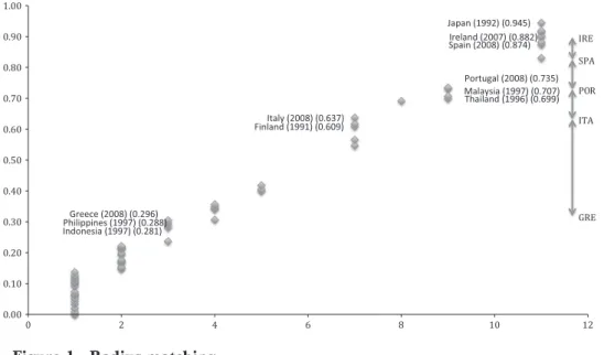
Between pairs Distance from Ireland Greece (0.296) Philippines, 1997 (0.288) Indonesia, 1997; Philippines, 1997 (0.281; 0.288) 0.008 0.586 Italy (0.637) Finland, 1991 (0.609) Norway, 1987; Finland, 1991 (0.566; 0.609) 0.028 0.245 Portugal (0.735) Malaysia, 1997 (0.707) Thailand, 1996; Malaysia, 1997 (0.699; 0.707) 0.028 0.147 Spain (0.874) Japan, 1992 (0.945) Japan, 1992 (0.945) 0.071 0.008 Ireland (0.882) 0.063 . . .
(new crises) and control (old crises) groups. Making use of this metric one could add to the qualitative discussions from matches by discussing the distance between each pair of new-old crises. Columns (4) and (5) of Table 4 provide this information. In column (4), we report the distance between each new-old pair, providing information on how relatively distant these crises are. The distance of the match between the crises of Greece (2008) and the Philippines (1997) at the level of 0.008 is much less than the dis-tance between the crises of Spain (2008) and Japan (1992) at the level of 0.071. This distance metric indicates the economic similarity of the Greece and Philippines crises is much greater than that of the Spain and Japan crises.
In column (5), we report the distance between the GIIPS crises, providing a metric of how similar the GIIPS crises are among themselves. The distance of each crisis is measured from the case of Ireland as a benchmark. Two results stand out. The ongoing crisis is not a single GIIPS crisis; each crisis within the GIIPS countries is unique in itself. However, the GIIPS group also has sub-clusters. The crises of Spain and Ireland are almost identical in this metric but are quite apart from the crisis of Greece. Indeed, the crisis of Greece separates very strongly from the remaining GIIPS crises. The distance between the GIIPS crises is graphically represented on the right-handside of Figure 1, showing the dissimilarity of the crisis in Greece from the remainder of the GIIPS crises.
While the one-to-one matching allows for a discussion of individualized pairs, addi-tional information can also be obtained from a radius matching exercise. The results of this radius matching are reported in Figure 1, with special focus on the GIIPS crises that are also summarized in column (3) of Table 4. While the one-to-one matching allows for the discussion of the existence of a match, the radius matching allows for
discussion of matches that fall within a range, which makes it possible to quantify the degree of similarity within the matches in a group.
Each group of data presented in Figure 1 represents the matched old and new crisis within the radius. The data is divided into eleven sets of matches, four of which include matches with the GIIPS countries. The one-to-one matches of the GIIPS countries were so distinct from each other that the clusters are robust to the method of matching used. Even after carrying out a radius matching the GIIPS countries remained in distinct matched groups. This result reinforces the finding that rather than consider a single periphery European crisis, it is necessary to take each individual crisis on a case-by-case basis.
Even though the GIIPS crises continue to remain apart in radius matching, several of the GIIPS crises are found to share similarities with more than one old crisis. Therefore, the extended clusters allow for a better understanding of the nature of the ongoing crisis. For example, while the 1997 Philippines crisis is found to be the most similar crisis to the ongoing crisis in Greece, the radius matching analysis allows us to also add the 1997 Indonesia crisis as another close match too. As such, the wealth of information available to better understand the ongoing crisis increases. Similarly, while the crisis in Malaysia (1997) is found to share the most similarities with the ongo-ing crisis in Portugal, results suggest that the crisis in Thailand (1996) is also relatively similar.
Overall, the propensity score matching suggests that despite their distinctive struc-tural characteristics and the global conditions during which they experienced a crisis, the domestic vulnerabilities leading up to their respective crisis shows sufficient com-monalities between the GIIPS countries and several earlier crises.12Results further-more indicate that there is no sui generis periphery euro crisis. Each country crisis in the periphery is different from each other. Table 4 presents clear statistical evidence that what the euro periphery has been experiencing since 2007/8 is not a single crisis. The variation of crises within the periphery is very large. The results of the radius matching that is illustrated in Figure 1 reflects this high variation – the individual GIIPS crises are far apart from each other (except for Ireland and Spain), and there is clustering in different subsets.
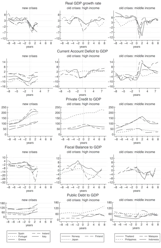
Keeping in mind the multidimensionality of factors that contribute to the matches, it is possible to discuss the similarities and discrepancies of the pre- and post-crisis experiences of the matched cases. Figure 2 provides a visual aid by plotting each domestic vulnerability variable included in the matching exercise, where the crisis year is taken as time zero and the period preceding it is referred to as pre-crisis and the period proceeding it is referred to as post-crisis.
12
The analysis was also conducted by including all three dimensions simultaneously in the propensity score estimation; however, the quality of match tests suggests against it. As such the three dimensions are analysed separately.
While the EMU project unified countries in the use of a common currency, speaking of a single eurozone continues to be an issue that is unsettled among policymakers and academics. The convergence of several economic indicators in the early years of the latter half of 2000s seemed to support the idea that there was actually a single eurozone. This convergence quickly turned sour with the onset of the banking crisis. The bond yields started decoupling once again.13 The external imbalances within Europe became a central point of discussions. Similarly, the internal imbalances reflected in productivity-adjusted unit labour costs that lie at the core of these external imbalances within Europe are heard of increasingly. These differences across countries are also the underlying factors that contribute to the observed matches of GIIPS countries with past crisis experiences, as provided in the following discussion.
3.4. Case 1: Portugal (2008)– Malaysia (1997) and Thailand (1996)
The prospects of entering Euro fuelled an average per annum growth rate of above 4% in Portugal in the second half of the 1990s. However, this growth was short-lived. After peaking at 5.2% in 1998, the Portuguese growth rate started decreasing steadily, leading to what Blanchard (2007) and Reis (2013) term the Portuguese slump. This slump period is marked by low productivity growth, and a loss of competitiveness on account of increases in nominal wages. Together with a drop in public savings, this loss in competitiveness reflected itself in a worsening current account deficit.
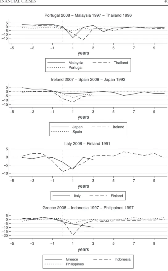
The pre-crisis growth patterns of Portugal and Malaysia or Thailand, on the other hand, differ significantly. The per annum average growth rate in the five years preced-ing the crisis was around 9.5% for Malaysia and 8.6% for Thailand. However, unlike the pre-crisis period, the growth patterns of Portugal and Malaysia and Thailand share a significant amount of similarities immediately after their respective crises (Fig-ure 3). The imbalances in both Malaysia and Thailand were corrected immediately after the crisis hit. With the help of significant real devaluation (around 30%) of their currencies, accompanied by countercyclical fiscal policies in both countries and rapid bank restructuring policies, Malaysia and Thailand experienced growth rates close to their tranquil period experiences within two years of their crises.
In comparison to Malaysia and Thailand, Portugal has experienced a smaller amount of decline in its growth rate relative to its tranquil period growth rate. As such, the necessary real exchange rate adjustment seems to be less than what Malaysia and Thailand needed in 1996/7. However, regardless of the level of adjustment that is necessary what is important is that Portugal needs to pursue policies that will hasten the real exchange rate devaluation.
13
While their growth performances did not resemble the strong slowdown of Portugal in their respective pre-crisis periods, the current account imbalances of Malaysia and Thailand showed strong resemblance to Portugal in their respective pre-crisis period. Among the GIIPS countries up until two years prior to the crisis, the current account imbalances in Portugal were the worst. Similarly, among the Asian-5 countries Malay-sia and Thailand were experiencing the worst current account imbalances two years prior to their 1996/7 banking crisis. This similarity is reflected in the close match of the pre-crisis conditions of the ongoing crisis in Portugal with the 1996/97 banking crises of Malaysia and Thailand.
Alongside the external imbalances, the evolution of private sector credit also shows significant similarities between Portugal, Malaysia and Thailand in their respective pre-crisis periods. Among the GIIPS countries, Portugal had the highest share of pri-vate sector credit to GDP ratio 5–8 years prior to the current crisis. However, despite this high initial level, the rate of expansion of private sector credit was much slower in Portugal than it was in Ireland or Spain. This pattern closely matches that of the Jap-anese, Malaysian and Thai private sector credit-to-GDP ratios prior to their respec-tive banking crises that started in 1992 and 1997, respecrespec-tively. The highest private sector credit-to-GDP ratio was experienced by Japan among the control group, followed by Thailand and Malaysia. The average private sector credit-to-GDP ratio for Thailand and Malaysia was around 100% in the years prior to the banking crisis, whereas for Indonesia and the Philippines it was around 30%.
The economic activities that were financed by the expansive private sector credit also showed discrepancies across the GIIPS countries. While the increasing credit was channelled into the real estate market in Spain and Ireland, in Portugal households preferred financial asset holdings to real estate investments. This difference is what possibly causes the Portuguese crisis to fall into a different radius set from Spain and Ireland.
3.5. Case 2: Spain (2008)– Ireland (2007) – Japan (1992)
Unlike Portugal, Spain and Ireland experienced high growth prior to the 2007/8 cri-ses. In both countries, this growth was fuelled by the construction sector on account of a housing boom. Financial market intermediation focused mainly on the financing of the demand for real estate. The growth in the construction sector also contributed positively to the employment patterns, lowering the unemployment rates. This cycle is no different from the asset bubble experienced by Japan in the latter half of the 1980s, running into the 1992-banking crisis. Asset prices, especially real estate and stock prices, were very high and increasing.
The credit expansion that contributed to the asset price increases show strong sim-ilarities between Japan, Ireland and Spain prior to their respective crisis experiences. In all three cases the share of private sector credit in GDP was well above 100% on
average in the 10 years preceding the crisis. This ratio was 108% for Ireland, 112% for Spain and 132% for Japan in their respective pre-crisis years.
A similarity is also evident in the real GDP growth performances of the three countries. In the 10 years preceding the banking crisis of 2007, the Irish real growth rate per annum was above 6%, the Spanish growth rate was around 3.85% while the Japanese growth rate was around 4.5%. Taking into account the growth rates of other high-income countries allows all three pre-crises cases to be classified as high-growth cases. However, one difference in these three cases is that the real slow-down was initiated much earlier in Japan when compared to Spain and Ireland.
While there are strong similarities in the economic performance and the source of growth in all three countries prior to their crises, the external imbalances of the three countries show divergent patterns. Ireland, having run a current account surplus from 1991–99 started running a current account deficit in 2000. This deficit continued increasing throughout the 2000s, the period of cheap international/intra-EU fund availability. Spain started running current account deficits in 1987, remaining much below 3.5% throughout the 1990s. However, the availability of increased inter-national funds in the 2000s accompanied by the domestic demand for construction reflected itself in a sharply increasing current account deficit trend. Right before the 2008 crisis the current account deficit of Spain had reached 10% of its GDP. While Spain and Ireland show a strong resemblance in their current account dynamics, Japan shows a strong dissimilarity from both cases, steadily running a current account surplus.
The similarity in financial sector outweighs the dissimilarity in the dynamics of the current account in providing important information regarding the matching of these crises. The exuberant domestic credit expansion that fuelled the property bubble is what matters in understanding the matching of the three cases.
The commonality of the pre-crisis conditions for Ireland and Spain with Japan could be worrisome given the lost decade Japan experienced in the subsequent years (Figure 3). Among the main culprits of this lost growth, Hoshi and Kashyap (2004, 2011) point to the lack of sufficient financial sector reforms. The financial deregulation that started in the mid-1970s, they argue, not only contributed to the build up of the asset bubble that led to the crisis but also created hindrances to the growth prospects of Japan by eliminating any incentive for creative destruction during the lost decade. An in-depth financial sector reform that would eliminate the non-performing loans and lending to what they call ‘zombie firms’ is put forth as a necessary policy to increase the efficiency of financial intermediation (Cabal-lero et al., 2008).
The same time period was marked by expansionary fiscal policies. However, despite its expansionary nature, the composition and content of the fiscal policy was not effective (Doi and Ihori, 2009). Excessively inefficient spending pro-grammes not only led to misallocation of resources, and hence created a hindrance
to growth, but also contributed to a continuous build-up of fiscal imbalances. The significant build-up in the public debt of Japan in the post-crisis period is evident in the steep upward trend of the public debt-to-GDP ratio depicted in Figure 2.
While both Spain and Ireland have been emphasizing the restructuring and resolu-tion of banks (OECD, 2013), there might still be issues that need attenresolu-tion in light of the Japanese experience. For example, non-performing loans continue to increase in Ireland, an issue that bears similarities to Japan’s post-crisis period experience at the aggregate level. However, the fiscal implications and burdens this could create on creditors generate a tension that requires a balancing of actions. Furthermore, in the absence of independent monetary policy and fiscal limitations due to euro membership, compared to Japan’s case, Ireland and Spain have less room for manoeuvre.
On the fiscal front, both Spain and Ireland have consolidated their fiscal positions over the past four years; the cyclically adjusted fiscal deficit decreased from 11.9% of GDP in 2008 to 6.9% of GDP in 2011 in Ireland, and from 7.1% in 2009 to 3.0% in 2011 in Spain. What seems more relevant in light of the Japanese experience is, how-ever, the quality of the fiscal balances. In Spain’s case, for example, the role played by regional governments in the overall fiscal balance is an important issue that should accompany any fiscal policy decision at the aggregate level.
3.6. Case 3: Italy (2008)– Finland (1991)14
This match is, at first sight, the one that is most unexpected. However, the slow-down in Finland prior to the deep systemic banking crisis incidence and the low levels of economic activity in Italy, their respective levels of the private sector credit and the transmission of global slowdowns via international trade linkages are common features of the slowdown in Italy in 2008 and the banking crisis of Finland in 1991.
Preceding the global financial crisis, Italy, like Portugal, had been experiencing a low growth period. The average annual growth rate of Italy in the decade prior to the outset of the current banking crisis was just 1.5%, even lower than the 2% Portugal experienced. The structural problems that underlie this sluggish growth rate in Italy are well documented in the literature. However, it made the current account dynam-ics very manageable. This is contrary to the case of Finland, except for the year prior to the banking crisis, during which the overheated Finnish economy had already started slowing down.
Prior to its systemic banking crisis in 1991, Finland experienced years of economic boom that was on account of significant debt accumulation made possible by financial
14
Although Norway’s crisis also matches with that of Italy, due to the significance of the developments in the oil market for the case of Norway it is excluded from the remainder of the discussions.
deregulation. The financial deregulation led to capital inflows and a fast expansion of domestic credit that fuelled domestic consumption. However, despite this rising trend in private sector credit, a closer look into the numbers is suggestive of why the Italian experience of 2008 matches that of Finland in 1991. The evolution of the private sector credit prior to their respective economic slowdowns in 2008 and 1991 show a strong resemblance.
One other strong similarity between the two cases is that in both there is a robust transmission of global events through real economic activities. In the case of Finland 1991, the hike in German interest rates on account of the reunification and the col-lapse of bilateral trade flows with the Soviet Union contributed significantly to the economic slowdown (see Honkapohja and Koskela, 1999). In Italy a similar real trans-mission of a global financial crisis was experienced, where a strong recession in its main trading partners led to a strong drop in exports, contributing to one of the worst recessions in the country since World War II.
In dealing with the crisis, Finnish authorities raised the interest rates to protect the currency, Markka. However, this policy was not enough to stave off the pressures on the currency. Eventually, the authorities decided to devalue the Markka in 1991. Realizing devaluation was not enough to correct the imbalances, in 1992 they finally allowed the Markka to float. The total loss in the real value of the Markka over these two years was around 35%.
At the onset of its crisis, Finnish fiscal policy carried countercyclical features. How-ever, in 1992 the fiscal policy was tightened and it remained unchanged throughout 1993. This policy formulation prioritized the sustainability of the fiscal position despite the cost of increasing unemployment. The combination of these policies con-tributed to a recovery path, and Finland was able to achieve growth rates above its tranquil period in the third year of the crisis.
Italy, sharing sufficient commonalities with Finland at the onset of the crisis, how-ever, has not been able to implement a strong real depreciation. From 2008 to 2011 the real exchange rate loss for Italy was limited to 2%. The Italian authorities announced fiscal policies aimed at consolidating the deficit. These policies resulted in a decrease of the cyclically adjusted primary balance as a share of GDP from 4.1% in 2009 to 3.5% in 2011.15Despite these differences in the ingredients of the policy mix, Italy’s growth pattern in the first two years of the crisis remained very similar to that of Finland. However, this trend seems to have broken in the third year of the crisis. While Finland’s growth pattern was on a positive trend, Figure 3 depicts a reversal of this pattern for Italy.
This reversal coincides with the divergence of the crisis experiences of Finland and Italy. Around this time the Italian crisis was no longer perceived as a financial crisis but had transformed into a sovereign debt crisis. Conversely, the crisis in
15
Finland did not evolve into a debt crisis. This divergence in their growth paths could possibly shed light on the importance of fiscal sustainability. In its post-crisis policy framework, Finland emphasized fiscal sustainability as part of its recovery package and benefitted from a recovery that allowed for growth above its tranquil period averages.
3.7. Case 4: Greece (2008)– Indonesia (1997) – The Philippines (1997)
Prior to the onset of the recent banking crisis, Greece was growing in a similar fashion to Spain. With the aid of cheap EU funds and the benefits accruing from the monetary union, Greece was able to increase its consumption through borrow-ing. Both the private and the public sector were heavily involved in this borrowing process.
The repercussions of this debt-driven-consumption behaviour reflected itself in the largest fiscal imbalance among the GIIPS countries, at an average of around 7% of its annual GDP for 1990–2007. This is much higher than the annual average for Ireland (0.1%), Italy (5.4%), Portugal (5%) or Spain (2.3%) over the same period (Figure 2). This corresponded to a very high public debt to GDP ratio, and a steadily rising one since 2007 (Figure 2).
The inflow of funds, however, was not intermediated to the private sector through the financial system, as is evident in the lowest private sector credit-to-GDP ratio among the GIIPS countries. Indeed, it is this feature of the Greek experience that leads to its match to Indonesia and the Philippines 1996–97 banking crisis experi-ences. Although the fiscal pre-crisis conditions show strong dissimilarities, the domestic credit dynamics show such a strong resemblance that the Indonesian and Philippines banking crises are found to share sufficiently large commonalities in their pre-conditions with Greece.
The growth trajectories in Indonesia and the Philippines differed in the post-crisis period, and this difference bears significant policy implications. The most important difference between the post-crisis period of Indonesia and the Philippines is that there is a level difference in the growth trajectory of the two countries although they share a similar pattern. This difference, which is reflected in a significant contraction in Indo-nesia compared to the Philippines, is on account of the political instability IndoIndo-nesia experienced in 1998. The additional loss in growth on account of the political instabil-ity meant the policy choices of Indonesia and the Philippines would differ drastically, even though they share significant commonalities pre-crisis (Figure 3).
The stronger contraction in Indonesia created the need for a stronger real exchange rate devaluation compared to that of the Philippines. The recovery of Indonesia required that the Rupiah lose more than 50% of its value in real terms, a very high figure when compared to the approximately 20% real loss in the value of the Philip-pine Peso. Given that the growth performance of Greece is still to reach its trough and its level remains between those of Indonesia and the Philippines, these figures
provide a benchmark range for the necessary real exchange rate adjustment for Greece.
The smaller contraction in the Philippines, on the other hand, generated room for manoeuvre in terms of fiscal policy choices, once again creating diverging paths for the two countries. Given its limitations in raising resources and funds, due to the strong contraction, Indonesia had no option but to follow more contractionary fiscal policies that were part of the IMF lending programme. However, since the Philippines had room for manoeuvre, it followed Keynesian countercyclical fiscal policies.
This room for manoeuvre was also made possible thanks to the much lower accu-mulated public debt figures in the Philippines. Throughout the post-crisis period the public debt in the Philippines ranged between 50% and 60% of its GDP. On the other hand, despite going into the crisis with much lower public debt ratios, once the crisis occurred, the share of Indonesia’s public debt increased from 26.4% in 1997, to 72.5% in 1998 and to 95.9% in 1999. The fiscal sustainability issues raised by this trend constrained Indonesia’s fiscal policy options and may have contributed to the divergence in the fiscal policy choices among the Philippines and Indonesia.16
In this regard, Greece shares more similarities with Indonesia than it does with the Philippines. Greece entered the crisis with an already very high public debt ratio, which further picked up pace throughout the crisis to increase from 107.4% of its GDP in 2007 to 165% of its GDP in 2011. The increasing intolerance of debtors in financing its ever-increasing public debt is evident in the accompanying rise in its borrowing cost spread. Therefore, one could interpret this as suggesting that Greece’s current situation is similar to Indonesia in the late 1990s. While one is an advanced country and the other is an emerging market, both faced debt-intol-erant lenders. Given the same fiscal sustainability concerns with Indonesia, it is highly probable that Greece will continue facing similar constraints in freely choos-ing its fiscal policy. With limited resource-generatchoos-ing means, it is more probable that Greece will be unable to put aside the contractionary fiscal policies, and will share a growth experience that resonates with that of Indonesia rather than the higher-level growth experience of the Philippines. However, for a comparison with Indonesia one should further be reminded that the Indonesian experience was accompanied by a strong real devaluation.
4. POLICY CONCLUSIONS
The above discussion provides a depiction of how similar each individual euro peri-phery crisis is to an earlier banking crisis. Given that these earlier crises have already
16
What Indonesia experienced is actually the reflection of what is referred to as the debt intolerance phe-nomena by Reinhart et al. (2003). During the 2000s many of the GIIPS countries had public debt ratios much higher than that of Indonesia in 1998, and did not have difficulty in generating resources.
Table 5. Summary statistics for cost of crisis Variable No. of crisis Mean Japan, 92 Thailand, 96 Malaysia, 97 Indonesia, 97 Philippines, 97 Norway, 87 Finland, 91 Years in crisis 165 3.84 10.00 6.00 5.00 6.00 5.00 7.00 5.00 Real GDP growth rate 159 1.18 0.84 0.90 3.09 0.90 3.00 1.99 –0.54 Real GDP growth rate deviations from tranquil periods 148 –2.45 –1.77 –6.24 –3.86 –5.40 –1.29 –0.77 –3.50 Real consumption growth rate 128 0.84 1.71 1.63 3.21 2.66 4.13 1.21 –0.86 Real consumption growth rate deviations from tranquil periods 128 –3.66 –0.82 –4.46 –3.63 –2.95 0.06 –1.90 –3.84 Real investment growth rate 124 2.31 –1.01 –9.08 –3.20 –2.45 0.62 –2.38 –6.67 Real investment growth rate deviations from tranquil periods 124 –42.07 –4.15 –20.65 –12.67 –18.50 12.37 –9.63 –13.97 Real domestic demand growth rate 123 1.93 1.32 –1.06 1.33 2.06 3.89 1.27 –1.52 Real domestic demand growth rate deviations from tranquil periods 123 –42.49 –1.82 –12.64 –8.14 –13.99 –9.10 –5.98 –8.82 Real GDP growth rate, first four year of crisis 155 0.43 0.95 –0.38 3.74 –0.68 3.02 1.13 –1.66 Real GDP growth rate deviations from tranquil periods, first year of crisis 148 –2.45 –1.80 –1.23 0.36 –1.61 0.89 –0.98 –8.97 Note s: Own calcula tions. Variabl e aver ages for duration o f each individual crisis. Domes tic deman d is the sum of con sump tion, investm ent and public spendi ng .
come to an end and completed their terms, they provide a wealth of information on how such crises evolve and what role policies might play in the process.
Table 5 provides an overview of the evolution of the older crises. What is strik-ing is the length of these matched older bankstrik-ing crises. The duration of these old crises are significantly longer than the average banking crisis for the whole sample. This has important implications for the new crises: the old crises they share com-monalities with have experienced much more prolonged crisis recoveries than the average experience.
Alongside the duration of a crisis, indicators that depict the change in economic activity are also reflective of how the crisis evolves. We follow Gupta et al. (2007), Lane and Milesi-Ferretti (2010) and Rose and Spiegel (2011) in defining the crisis intensi-ties. Namely, we measure crisis intensities (severity) by either the average growth rate during the crisis years, or the difference of this growth rate from the average over the tranquil period, the years during which the economy does not experience a financial crisis.17
As is shown in Table 5, the crisis intensities of matched cases differ. The real GDP growth rate is lower on average during the episode of crisis in Japan compared to the sample average, while it is higher for the Philippines and Malaysia during their crisis episodes. The deviations of the average growth rate in each country relative to their tranquil period also show a variation across countries.
What is more striking is how costly all of these matched old crises have been. Usually in the post-crisis periods, despite significant output losses, economic growth itself recovers. However, in the majority of the matched old crises the growth rates remain below their tranquil period averages over extended time periods (Figure 3). This is true even for periods that go beyond the dates identified as a crisis by Laeven and Valencia (2012) or Reinhart and Rogoff (2009). As depicted in Fig-ure 3, taking a 14-year window around the crisis, the growth rate remains below that of tranquil periods for very long time periods.18 Indeed, over the 14-year time frame, in Japan the growth rate is below the tranquil period average for 8 years. In other words, once Japan entered the crisis it remained there throughout the period of analysis.
This broad comparison depicts a strikingly difficult post-crisis period for the matched old crises. As such, at the aggregate level it is suggestive of what awaits the euro periphery countries. However, as the matching exercise has already ascertained, one should not discuss policies at an aggregate level, but should take into account the unique nature of each and every crisis. In the preceding section such an exercise was
17
Alternatively we also calculate these two measures using components of GDP, namely private con-sumption, private investment and total domestic demand. Given the high correlation among all of these alternative measures, in the remainder of the discussion we report results using the two crisis incidence measures based on the real GDP.
18
The 15 years include 4 years prior to the crisis, and 10 after the first year of the crisis (given that the Japanese crisis in our dataset is identified as being 10 years long).