Multilevel cluster ensembling for histopathological image segmentation

SEGMENTATION

a thesis

submitted to the department of computer engineering

and the graduate school of engineering and science

of bilkent university

in partial fulfillment of the requirements

for the degree of

master of science

By

Ahmet C

¸ a˘grı S¸im¸sek

August, 2011

I certify that I have read this thesis and that in my opinion it is fully adequate, in scope and in quality, as a thesis for the degree of Master of Science.

Prof. Dr. Cevdet Aykanat(Advisor)

I certify that I have read this thesis and that in my opinion it is fully adequate, in scope and in quality, as a thesis for the degree of Master of Science.

Assist. Prof. Dr. C¸ i˘gdem G¨und¨uz Demir (Co-Advisor)

I certify that I have read this thesis and that in my opinion it is fully adequate, in scope and in quality, as a thesis for the degree of Master of Science.

Prof. Dr. Fato¸s T¨unay Yarman-Vural

I certify that I have read this thesis and that in my opinion it is fully adequate, in scope and in quality, as a thesis for the degree of Master of Science.

Assoc. Prof. Dr. Hakan Ferhatosmano˘glu

Approved for the Graduate School of Engineering and Science:

Prof. Dr. Levent Onural Director of the Graduate School

HISTOPATHOLOGICAL IMAGE SEGMENTATION

Ahmet C¸ a˘grı S¸im¸sek M.S. in Computer Engineering

Supervisors: Prof. Dr. Cevdet Aykanat and Assist. Prof. Dr. C¸ i˘gdem G¨und¨uz Demir

August, 2011

In cancer diagnosis and grading, histopathological examination of tissues by pathologists is accepted as the gold standard. However, this procedure has ob-server variability and leads to subjectivity in diagnosis. In order to overcome such problems, computational methods which use quantitative measures are proposed. These methods extract mathematical features from tissue images assuming they are composed of homogeneous regions and classify images. This assumption is not always true and segmentation of images before classification is necessary. There are methods to segment images but most of them are proposed for generic images and work on the pixel-level. Recently few algorithms incorporated medi-cal background knowledge into segmentation. Their high level feature definitions are very promising. However, in the segmentation step, they use region growing approaches which are not very stable and may lead to local optima.

In this thesis, we present an efficient and stable method for the segmentation of histopathological images which produces high quality results. We use existing high level feature definitions to segment tissue images. Our segmentation method significantly improves the segmentation accuracy and stability, compared to ex-isting methods which use the same feature definition. We tackle image segmen-tation problem as a clustering problem. To improve the quality and the stability of the clustering results, we combine different clustering solutions. This approach is also known as cluster ensembles. We formulate the clustering problem as a graph partitioning problem. In order to obtain diverse and high quality cluster-ing results quickly, we made modifications and improvements on the well-known multilevel graph partitioning scheme. Our method clusters medically meaningful components in tissue images into regions and obtains the final segmentation.

iv

Experiments showed that our multilevel cluster ensembling approach per-formed significantly better than existing segmentation algorithms used for generic and tissue images. Although most of the images used in experiments, contain noise and artifacts, the proposed algorithm produced high quality results.

Keywords: Histopathological image segmentation, cluster ensembles, multilevel

H˙ISTOPATOLOJ˙IK G ¨

OR ¨

UNT ¨

U B ¨

OL ¨

UTLEMES˙I ˙IC

¸ ˙IN

C

¸ OK SEV˙IYEL˙I K ¨

UMELEME B˙ILES

¸˙IM˙I

Ahmet C¸ a˘grı S¸im¸sek

Bilgisayar M¨uhendisli˘gi, Y¨uksek Lisans Tez Y¨oneticileri: Prof. Dr. Cevdet Aykanat ve

Yrd. Do¸c. Dr. C¸ i˘gdem G¨und¨uz Demir A˘gustos, 2011

Dokuların patologlar tarafından histopatolojik incelemesinin yapılması, kanser

tanı ve derecelendirmesinde altın standart olarak kabul edilir. Bu i¸slemde

g¨ozlemcilerin de˘gi¸skenlik g¨ostermesi, tanı sonu¸clarında ¨oznelli˘ge sebep olur. Bu tarz sorunların ¨ustesinden gelebilmek i¸cin, nicel veriler kullanan hesaplamasal teknikler ileri s¨ur¨ulm¨u¸st¨ur. Bu teknikler, doku resimlerinin homojen b¨olgelerden olu¸stu˘gunu varsayarak bu resimlerden matematiksel ¨ozellikler ¸cıkarır ve resimleri sınıflandırır. Fakat bu varsayım her zaman do˘gru de˘gildir ve sınıflandırmadan ¨once resimlerin b¨ol¨utlenmesi gerekir. Resimleri b¨ol¨utlemek i¸cin ¸ce¸sitli teknikler ileri s¨ur¨ulm¨u¸st¨ur, fakat bu tekniklerin ¸co˘gu imgecikler ¨uzerinde ¸calı¸sır ve genel resimler i¸cin geli¸stirilmi¸stir. Son zamanlarda birka¸c algoritma doku resimleri b¨ol¨utlemede tıbbi bilgileri kullanmı¸stır. Bu tekniklerin y¨uksek seviye ¨ozellik tanımları ¸cok ¨umit vericidir. Ancak, bu teknikler b¨ol¨utleme safhalarında, ¸cok kararlı olmayan ve yerel ¸c¨oz¨umlere ka¸cabilen b¨olge b¨uy¨utme yakla¸sımını kul-lanmı¸stır.

Bu tezde, histopatolojik resimlerin b¨ol¨utlenmesi i¸cin y¨uksek kalite sonu¸clar ¨

ureten, verimli ve kararlı bir y¨ontem sunuyoruz. Doku resimlerini b¨ol¨utlemek

i¸cin var olan y¨uksek seviye ¨ozellik tanımlarını kullandık. B¨ol¨utleme y¨ontemimiz, bizimle aynı ¨ozellik tanımını kullanan di˘ger y¨ontemlerin b¨ol¨utleme ba¸sarısını ve kararlılı˘gını ¨onemli derecede arttırıyor. Resim b¨ol¨utleme problemini bir k¨umeleme problemi olarak kabul ettik. K¨umeleme sonu¸clarının kalitesini ve kararlılı˘gını arttırmak i¸cin farklı k¨umeleme sonu¸clarını bir araya getirip birle¸stirdik. Bu

teknik, k¨umeleme bile¸simi olarak da bilinir. Biz ayrıca k¨umeleme problemini

¸cizge b¨ol¨umleme problemine d¨on¨u¸st¨urd¨uk. Birbirinden farklı ve y¨uksek kaliteli k¨umeleme sonu¸cları elde etmek i¸cin, iyi bilinen ¸cok seviyeli ¸cizge b¨ol¨umleme

vi

tekni˘gi ¨uzerinde de˘gi¸siklikler ve iyile¸stirmeler yaptık. Y¨ontemimiz tıbbi olarak bir anlamı olan nesneleri ayrı b¨olgelere toplayarak sonu¸c b¨ol¨utlemeyi elde eder.

Yaptı˘gımız deneyler, ¨onerdi˘gimiz ¸cok seviyeli k¨umeleme bile¸simi tekni˘ginin,

genel resimler ve doku resimleri i¸cin daha ¨onceden ¨onerilmi¸s b¨ol¨utleme

tekniklerinden ¸cok daha iyi sonu¸clar ¨uretti˘gini g¨osterdi. Deneylerde kullandı˘gımız doku resimlerinin ¸co˘gu resim elde etme a¸samasında ortaya ¸cıkan bozulmalar i¸cermesine ra˘gmen, ¨onerdi˘gimiz y¨ontem y¨uksek kaliteli sonu¸clar ¨uretti.

Anahtar s¨ozc¨ukler : Histopatolojik g¨or¨unt¨u b¨ol¨utleme, k¨umeleme bile¸simi, ¸cok seviyeli ¸cizge b¨ol¨umleme, g¨ud¨ums¨uz b¨ol¨utleme .

I am grateful to my supervisors Prof. Dr. Cevdet Aykanat and Assist. Prof.

Dr. C¸ i˘gdem G¨und¨uz Demir for their guidance and support. I thank Prof. Dr.

Fato¸s T¨unay Yarman-Vural and Assoc. Prof. Dr. Hakan Ferhatosmano˘glu for

accepting to participate in my thesis committee.

I am also grateful to my colleagues Akif Burak Tosun, Erdem ¨Ozdemir, Ata

T¨urk, Tayfun K¨u¸c¨ukyılmaz, Enver Kayaaslan, Reha O˘guz Selvitopi, Kadir Ak-budak, and Fahreddin S¸¨ukr¨u Torun for their contributions and comments.

I present my thanks to Bilkent University and T ¨UB˙ITAK for supporting me

financially and physically.

Contents

2.1.5 Histopathological Image Segmentation . . . 14

2.2 Multilevel Framework . . . 15

2.3 Cluster Ensembling . . . 16

3 Methodology 19

3.1 Graph Construction and Feature Extraction . . . 20

3.2 Clustering . . . 22

3.2.1 Random Subsampling . . . 26

3.2.2 Multilevel Graph Partitioning . . . 27

3.2.3 Filling . . . 33

3.3 Consensus Function . . . 34

3.4 Post processing . . . 36

4 Experiments and Results 38 4.1 Experimental Setup . . . 38 4.1.1 Dataset . . . 38 4.1.2 Validation . . . 39 4.2 Results . . . 41 4.2.1 Parameters . . . 42 4.2.2 Comparisons . . . 45

List of Figures

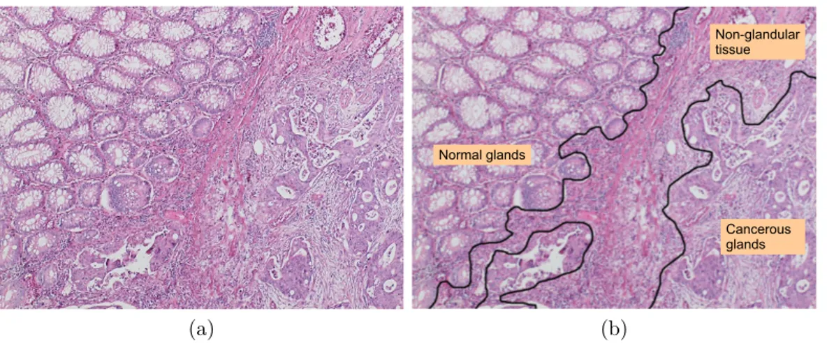
1.1 A colon tissue may consist of different types of regions: (a) a colon

tissue image and (b) its manual segmentation. . . 3

1.2 Heterogeneous histopathological images are composed of different

regions. . . 4

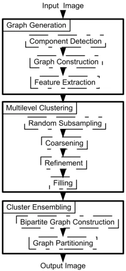
3.1 Overview of the proposed method . . . 20

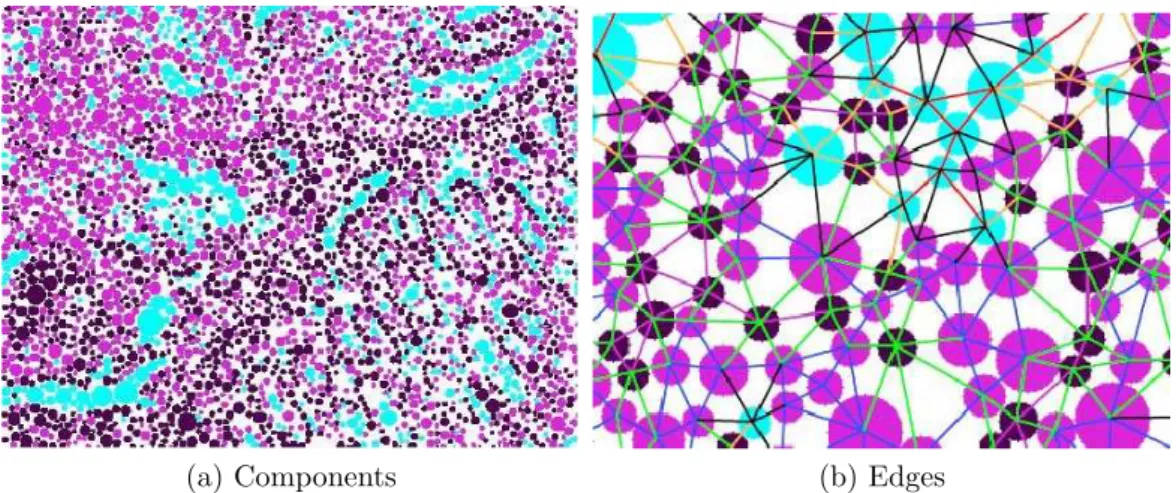
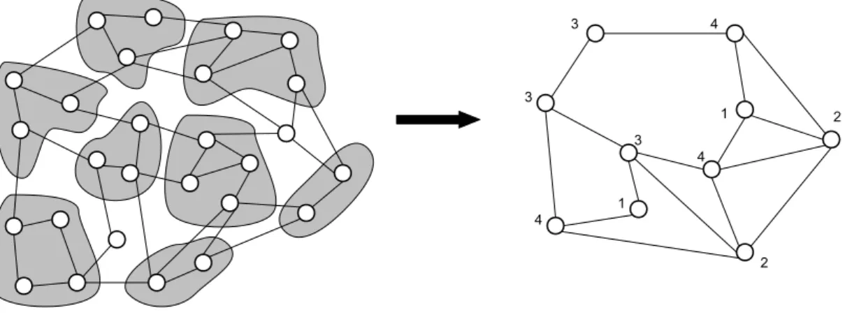
3.2 Detected tissue components(a). A close up view of some of the

edges found by Delaunay triangulation (b). . . 21

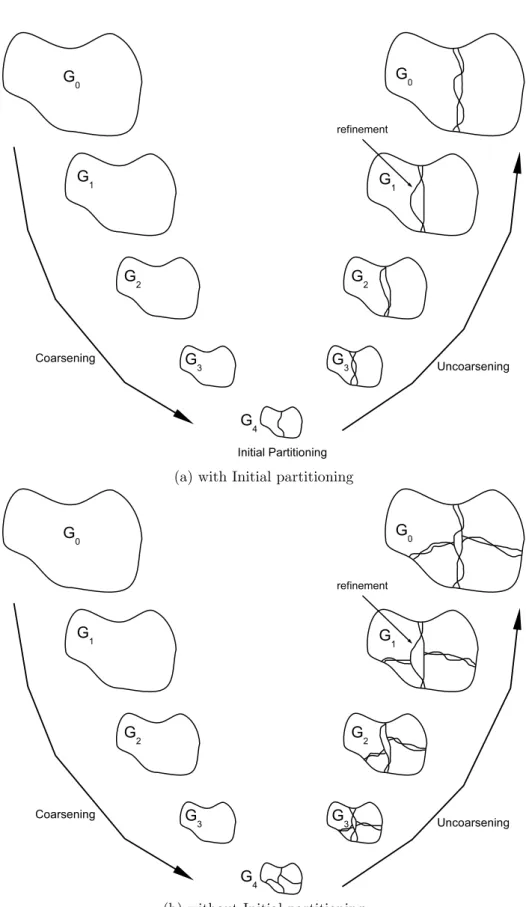
3.3 Multilevel Graph Bipartitioning with Initial partitioning (a).

Mul-tilevel Graph Partitioning without Initial partitioning (b). . . 25

3.4 Coarsening a graph . . . 27

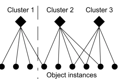
3.5 Bipartite graph representation of vertices and clusters . . . 35

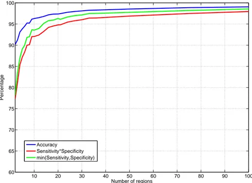
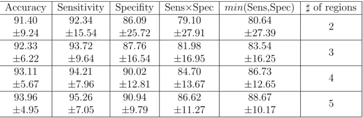
4.1 Segmentation performance increases as the number of regions

in-creases . . . 40

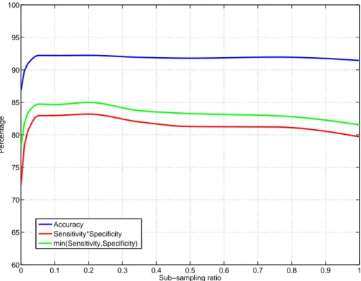
4.2 The segmentation performance of the test set as a function of the

sub-sampling ratio . . . 43

4.3 The segmentation performance of the test set as a function of the

initial K . . . 44 x

4.4 The segmentation performance of the test set as a function of the ensemble size . . . 45

4.5 Test results of the algorithms when the number of segmented

re-gions is fixed to 2 . . . 50

4.6 Test results of the algorithms when the number of segmented

re-gions is fixed to 3 . . . 50

4.7 Test results of the algorithms when the number of segmented

re-gions is fixed to 4 . . . 51

4.8 Test results of the algorithms when the number of segmented

re-gions is fixed to 5 . . . 51 4.9 Visual results for 2 example images: (a) gold standard for the first

image and it is segmented into (b) two, (c) three, (d) four regions. (e) Gold standard for the second image and it is segmented into (f) two, (g) three, (h) four regions . . . 54 4.10 Visual results for 2 example images: (a) gold standard for the first

image and it is segmented into (b) two, (c) three, (d) four regions. (e) Gold standard for the second image and it is segmented into (f) two, (g) three, (h) four regions . . . 55

List of Tables

4.1 The training results obtained by our multilevel cluster ensembling

(MLCE) algorithm . . . 41

4.2 The test results obtained by our multilevel cluster ensembling

(MLCE) algorithm . . . 41

4.3 Training results obtained by the algorithms. The results of the

proposed MLCE algorithm are reported for region no: 2, 3, 4, 5. For other algorithms, the results obtained when maximum 5 regions are selected. . . 48

4.4 Test results obtained by the algorithms. The results of the

pro-posed MLCE algorithm are reported for region no: 2, 3, 4, 5. For other algorithms, the results obtained when maximum 5 regions are selected. . . 49

4.5 Training results of the algorithms when the number of segmented

regions is fixed to 2 . . . 52

4.6 Training results of the algorithms when the number of segmented

regions is fixed to 3 . . . 52

4.7 Training results of the algorithms when the number of segmented

regions is fixed to 4 . . . 52

4.8 Training results of the algorithms when the number of segmented regions is fixed to 5 . . . 52

4.9 Test results of the algorithms when the number of segmented

re-gions is fixed to 2 . . . 53 4.10 Test results of the algorithms when the number of segmented

re-gions is fixed to 3 . . . 53 4.11 Test results of the algorithms when the number of segmented

re-gions is fixed to 4 . . . 53 4.12 Test results of the algorithms when the number of segmented

Chapter 1

Introduction

Cancer is a type of disease described by uncontrolled growth of abnormal cells. Damaged and abnormal cells reproduce uncontrollably and create masses of a tissue called tumors. Tumors can grow, distort, and change the cellular and or-ganizational structure of tissues from which they originate [1, 34, 45]. Metastasis occurs when a tumor spreads to different parts of the body, grows, invades, and destroys other healthy tissues. The result of metastasis is a serious condition which is very difficult to treat.

There are many types of cancer depending on the tissue it originates. Colon cancer is one of the most common cancers in the world [60]. Huge portion of cancer deaths are caused by colon cancer in the western world and in the coun-tries which adapted western diets. Although colon cancer has a high prevalence, the survival rate is high if it is diagnosed early and treated correctly. For the diagnosis of colon cancer, there are various types of screening tests such as dig-ital rectal exam, MRI, endoscopy, and colonoscopy. These tests mainly look for symptoms and polyps. If they locate polyps or find any other indicative symp-toms, histopathological examination should be conducted to confirm the cancer and its grade [31, 54]. In this examination, a small part of a tissue is extracted from a patient by surgery and examined under a microscope by pathologists.

Early detection and correct grading of cancer affect the success of the se-lected treatment method and increase the chance of survival [2]. Hence, using procedures that provide reliable information is very crucial. Histopathological examination is the most reliable procedure and considered as the gold standard for diagnosis and grading. In this examination, pathologists should be able to identify the changes in cellular structures and the deformations in tissue distribu-tion. This relies on visual interpretation of a tissue, and hence, is affected by the experience and expertise of pathologists [20, 77]. Moreover, tissue preparation procedures such as staining and sectioning operations may introduce noise and artifacts to the image, which makes the image hard to interpret [35]. Therefore, histopathological examination is subject to a considerable amount of intra- and inter-observer variability [43, 46, 12, 15]. In order to reduce the effect of observer variability, it is very important to standardize diagnosis and grading processes based on quantitative measures. One of the most reliable ways of doing this is to develop computational methods and build tools and programs.

1.1

Motivation

There are plenty of computational studies developed for histopathological image analysis. Most of these studies quantify histopathological images extracting their mathematical features and classify them based on the extracted features. These features include textural [21, 25, 26, 44, 66, 87], morphological [72, 73, 88], and structural [4, 86, 75, 22, 37, 38, 6] descriptors of the images. Although these de-scriptors are more or less successful to quantify homogeneous tissue images, they may fail to characterize heterogeneous tissue images, which consist of different homogeneous regions. As shown in Figure 1.1, colon tissue images may contain such regions that show very different characteristics in shape, color, and texture. Heterogeneity affects the representation power of the feature descriptors, and thus, the performance of classifiers. Segmenting heterogeneous tissue images into their homogeneous regions and then extracting the descriptors of these regions greatly improve the classification performance.

CHAPTER 1. INTRODUCTION ₃

(a) (b)

Figure 1.1: A colon tissue may consist of different types of regions: (a) a colon tissue image and (b) its manual segmentation.

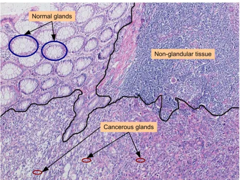
In histopathological images, regions are characterized with the organization of their components. A colon tissue is composed of glands. In a normal tissue, these glands follow a regular structure and colon cancer causes deformations in these structures. In addition to the regions containing normal and cancerous glands, there may also exist regions that do not contain any glandular structure. These types of regions are shown in Figure 1.2. In literature, there are many techniques for unsupervised segmentation of generic images. However, there are only few studies that have been proposed for histopathological image segmentation [71, 85]. These studies segment images dividing them into grids and classifying each grid based on its feature descriptors. These features are commonly extracted making use of pixel-level information, without considering the domain specific knowledge. Recently Tosun et al. [82, 81] introduced new sets of high level feature de-scriptors, which take medically meaningful objects into account. For that, they identify the approximate locations of cytological components in a tissue and de-fine the texture descriptors on these components instead of defining them on pixel values. Using these new descriptors, they achieve segmentation by a region growing algorithm. These studies [82, 81] aim to improve the segmentation per-formance by mainly focusing on the feature extraction part. On the other hand, there is a room of improvement in its segmentation part. Indeed, like all of its kinds, a region growing algorithm has a risk of obtaining a local optimal solution,

Figure 1.2: Heterogeneous histopathological images are composed of different regions.

especially when initial regions (seeds) are not carefully selected [90]. In this the-sis, we focus on improving the segmentation part. To this end, we propose a new algorithm that ensembles multiple segmentations. The experiments indicate that the proposed method is more effective to reduce the negative effects of finding local optimal solutions.

It is known for many years now that ensembles of different classifiers per-form better than a single classifier. Each classifier recognizes a different aspect of data and combining those multiple different points of views yields better ac-curacy. More recently, ensembling algorithms have been started to be used for clustering as well [74]. Single runs of clusterings may not be stable and may not yield accurate results for algorithms that require initialization points or that are randomized. Moreover, there may be cases, in which algorithms that can capture global optimum do not perform well under the conditions of noise and insufficient data representation. In such cases, the use of cluster ensembling has a potential to improve the results.

CHAPTER 1. INTRODUCTION ₅

result are the diversity and quality of individual clusterings [28, 52, 53]. In order to get an accurate and stable final clustering, each clusterer should yield an at least slightly different result to increase the diversity. There are several techniques to introduce diversity to clusterers. For that, it is possible to use a randomized version of the same algorithm. Alternatively, random subsets of data points or random subsets of features can be used to obtain each clusterer.

The quality of each clustering result should also be acceptably high. To this end, effective clustering algorithms should be used. Spectral methods are the examples of such algorithms [70, 57, 89]. In these methods, data points are con-sidered as graph vertices and similarity of these points correspond to weights of the graph edges defined between these data objects. The objective is to di-vide the graph into a predefined number of parts by minimizing the sum of the weights of the cut edges. This directly corresponds to the goal of the clustering problem where ”inter-cluster distance is maximized and intra-cluster distance is minimized”. These spectral methods perform considerably well in finding global optimum. However, as these algorithms need eigen decomposition, they are very demanding in both CPU time and memory space. Moreover cluster ensembling requires running these algorithms multiple times, which further increases the com-putational costs. To overcome the comcom-putational burdens of spectral methods, Dhillon et al. propose to use multilevel graph partitioning. They show that sim-ilar results can be obtained with multilevel graph partitioning by breaking the balance criterion [18, 47]. However their proposed algorithm is not a good choice for cluster ensembling since it usually yields lower diversity.

1.2

Contribution

In this thesis, our main contribution is as follows: We present a new multilevel cluster ensembling algorithm to be used in histopathological image segmentation. The proposed method is efficient and stable. It yields accurate segmentations avoiding local optimum and over-segmentation. It achieves this by producing

diverse and high quality clusterings and combining them efficiently. In this algo-rithm, we work on the objects described in [81] and use a set of features defined on these objects. After defining the objects and their features, the algorithm con-siders each object as a data point in a clustering problem and clusters the objects into the desired number of clusters. It runs a predefined number of iterations to get different clustering results and combines them into a final clustering solution. In each iteration, it takes a random subset of objects and clusters them using a multilevel graph clustering algorithm whose refinement phase is redesigned to obtain diverse and high quality clustering solutions. The algorithm combines these clustering solutions with a consensus function. The consensus function constructs a bipartite graph, making clusters and objects two groups of vertices and connecting each cluster to the objects it contains by a unit weight edge [29]. This bipartite graph actually holds the objects’ frequency of being together in the same cluster. After that, it partitions the bipartite graph to get the final clustering solution. Our experiments showed that the proposed multilevel cluster ensembling provides an effective image segmentation tool for histopathological tissue images and significantly increases segmentation accuracies of the previous approaches.

1.3

Outline of Thesis

The outline of this thesis is as follows. Chapter 2 summarizes previous compu-tational methods for generic and histopathological image segmentation. Chapter 3 provides detailed description of the proposed multilevel cluster ensembling al-gorithm. Chapter 4 gives the experimental setup and reports the segmentation results of the proposed algorithm. It also gives the comparison of the proposed algorithm with other algorithms. Chapter 5 includes concluding remarks and discussions.

Chapter 2

Background

This chapter presents previous studies on image segmentation and its applications to histopathological images. In the first section, we explain previous studies on generic and histopathological image segmentation. In the second one, we explain multilevel framework. In the last section, we explain clustering and cluster ensembling.

2.1

Image Segmentation

Image segmentation is described as the operation of dividing an image into non-overlapping and connected pixel groups or regions that are semantically coherent in a particular context. Image segmentation aims to transform the representa-tion of images and make them more meaningful and easier to analyze [68]. Pixels sharing certain visual characteristics are classified into regions. Pixels in each region are similar in an attribute or a computed feature, like intensity, color, and texture. Bordering regions are quite different according to the same char-acteristics [68]. Image segmentation is a well studied subject in computer vision and attracted a great deal of attention by many researchers. As a result, there are lots of different algorithms and approaches for image segmentation. These

can be grouped into four: pixel-based methods, graph-based methods, region-based methods, and statistical methods. In the following subsections, we briefly mention these methods.

2.1.1

Pixel-based Methods

Pixel-based methods consider pixels as the smallest informative part of the image and groups the pixels according to their intensity or color values using different techniques.

2.1.1.1 Thresholding

Thresholding is the oldest and simplest segmentation method. It classifies pixels as foreground and background according to their intensities. For example, for detecting lighter foreground objects in darker background, a pixel is labeled as foreground object if its pixel value is greater than some threshold and as back-ground otherwise. Thresholding methods are generally the most efficient methods in terms of computational requirements. Otsu [58] has a seminal work, in which he proposed a statistical threshold determination method for grayscale images. Thresholding can also be used for color images. A separate threshold can be defined for every RGB component and then the thresholding result of each com-ponent can be combined with an AND operation. The HSL, HSV, and CMYK color models can also be used [61].

2.1.1.2 Edge Detection

Another method that works on pixel values is edge detection. Here segmentation is achieved by finding the region boundaries with an edge detection algorithm. In order to locate edges, changes in gray-level pixel values can be detected using first order derivative operators like Sobel and Prewitt and second order derivative operators like Laplacian [36]. As these operators are more sensitive to noise, it

CHAPTER 2. BACKGROUND ₉

is also possible to use operators such as Laplacian of Gaussian and difference of Gaussians. For example, the Laplacian of Gaussian operator first smooths an image with a Gaussian filter to reduce noise and then applies the Laplacian operator [55]. Another way is to use the Canny edge detector [10], which is a multi stage algorithm for edge detection.

2.1.1.3 Clustering Methods

Image segmentation is very similar to clustering in a sense that both try to group similar pixels or data points into groups according to a distance criterion. The simplest and the well known clustering technique is the k-means algorithm [32]. K-means first initializes the centroids of k clusters, randomly or using a heuristic. It then updates these centroids iteratively, until there is no significant change in the centroids. In each iteration, every data point is assigned to its nearest centroid and the new centroids are computed by averaging the data points that are assigned to those centroids. The k-means algorithm does not guarantee global optimum but good centroid initializations may lead to good results. An image can be segmented into regions by extracting intensity, color, and texture descriptors for each of its pixels and using the k-means algorithm [14, 9].

Fuzzy c-means [24] is another clustering algorithm used for image segmenta-tion [65, 13]. The fuzzy c-means algorithm introduces fuzziness to memberships of data points. Each data point belongs to every cluster with a weight coefficient, which gives the degree of that object being in a cluster. The fuzzy c-means al-gorithm is a slightly modified version of the k-means alal-gorithm with fuzziness. Just like in k-means, initial c cluster centroids are selected and then updated iteratively. In each iteration c weight coefficients are computed for each point. The coefficients are defined using a function of the distance between the point and the corresponding centroid. Once coefficients are found, cluster centroids are updated averaging the data points according to their weight coefficients.

The mixture of Gaussian model can also be used for clustering. In that case, maximum likelihood estimations of the covariances, means, and coefficients of

the model are computed iteratively. This model is more sensitive to initialization [16]. Clustering algorithms can be sensitive to noise and intensity heterogeneities, because they do not incorporate spatial information.

2.1.2

Region-based Methods

Region-based methods group image pixels into regions preserving spatial connec-tivity among the pixels in the same region.

2.1.2.1 Watersheds

Gray level intensity images can be segmented by watershed algorithms [5, 84]. These algorithms consider a gray level image as a topographic map and a pixel’s intensity value as its altitude in the map. A local minimum is the place where a drop of water falling on the topography flows down and finally reaches. A local minimum is the base for a catchment basin. Watersheds are the meeting points for the waters of adjacent catchment basins. In image segmentation, wa-tershed lines correspond to the region boundaries. There are several approaches to segment images using watershed representation. In one of them, a downstream path is first found from each image pixel to a local minimum point of surface al-titude of image. The set of pixels whose downstream paths meet in the same minimum altitude, is then defined as a catchment basin. Another approach uses flooding, in which the catchment basins are filled from the bottom, instead of characterizing the downstream paths. The barriers where water from different catchment basins meet are the watershed boundaries. Watershed methods are usually applied to gray level images and they suffer from the over-segmentation problem, which occurs when the number of regions in segmentation is higher than expected. Marker controlled watersheds are effective to alleviate the over-segmentation problem. These watersheds determine markers (flooding points), which correspond to local minima,at the beginning and allow rising the water only from these points.

CHAPTER 2. BACKGROUND ₁₁

2.1.2.2 Region Growing

Region growing methods extract regions that are composed of connected prim-itives with respect to some criteria [50, 17, 78, 3, 67, 79]. It is based on the assumption that neighbouring pixels have similar values. Seeded region grow-ing [3] is a common form of region growgrow-ing methods. Seeded region growgrow-ing is a semi-supervised method because it takes a group of initial seeds as an input. The seeds determine different regions to be segmented. Each region (seed) is grown iteratively by checking unlabeled neighboring pixels. Decision to include a neighbor pixel in the growing region is made on the similarity between the feature value of the neighbor pixel and the average of pixels in the region. The most similar pixel is included in the region in each iteration. Iterations continue until all pixels are labeled. One disadvantage of the method is the requirement of supervised inputs for the seed points. Therefore, for every region that is to be segmented, a seed point is necessary. There are also methods, in which seeds are automatically determined. The JSEG algorithm [17] is one of them. It defines J value for image pixels and identifies pixel groups with smaller J values as seeds. It is also possible to use approaches start with a single seed and add new seeds if necessary. These approaches apply the same operations on the neighboring pixels with the seeded region growing approaches. Differently, they include the neighboring pixel into the region if the similarity is above a threshold. If not, a new region is created with this neighboring pixel being a seed. Region growing techniques are similar to greedy algorithms that consider the best local choices at a given time. For this reason, they may lead to local optima. Region growing techniques are also computationally expensive.

2.1.2.3 Split-and-merge

Split-and-merge methods segment an image by recursive partitioning. The image is represented as a quadtree and each segment is partitioned into four equally sized squares. Split-and-merge methods start from the root of the tree. If it finds a heterogeneous region, it splits that region into four equal squares. If four equal squares are homogeneous, it can merge them as a connected component. This

operation is carried out recursively until no further splits or merges are possible.

2.1.3

Graph-based Methods

Graph-based methods construct a graph from a given image, where vertices rep-resent pixels and the edge weights reprep-resent the similarity between two connected vertices. They then consider the image segmentation as graph partitioning. There are algorithms solving this problem using different similarity measures, different cost functions, and different optimization methods.

Graph partitioning, clustering, and image segmentation are all similar prob-lems; they all partition the data into uniform groups. The first step to consider in solving these kind of problems is to define a criterion to optimize. The second step is to find an algorithm to carry out the optimization. Most of the time, the second step is more challenging and many attractive criteria suffer from the lack of an effective algorithm that finds the global optimum. Greedy or gradient de-scent based approaches usually fail to find global optimum for high-dimensional, non-linear problems. Therefore, algorithms that guarantee the global optimum are important as well as optimization criterion.

In graph-based approaches, the constructed graph can be divided into two separate parts by removing edges that connect the two parts. The distance be-tween these two parts is defined as the sum of the edge weights that are to be removed. This is called the cut in graph theory literature. The optimal bisec-tion of a graph, minimizes the cut value. Graph partibisec-tioning schemes partibisec-tion the graphs into a predefined number of vertex groups by optimizing the mini-mum cut criterion. This can be achieved by recursively computing the minimini-mum cuts bisecting the current regions. The minimum cut criterion may produce very small sized sets of vertices in the partition. This situation is expected, because the cut value increases with the increasing number of edges of boundary vertices. To avoid the unnatural bias for dividing small groups of points, Shi and Malik [70] propose a new measure. They find the cut as a ratio of the total edge con-nections to all graph vertices, instead of looking at the value of the sum of the

CHAPTER 2. BACKGROUND ₁₃

edge weights that connect the two parts. This is called the normalized cut. With their definition of the association between the different parts, the cut that divides small isolated points will not have a low normalized cut value. Because the cut will be a large fraction of the total edge connections from that little group to all other vertices. Minimizing normalized cut exactly is NP-complete. However, Shi and Malik propose an approximate discrete solution, which uses eigenvector decomposition. They construct the affinity matrix, which is the adjacency ma-trix of the graph, and solve the generalized eigenvalue problem for the normalized Laplacian of the affinity matrix. They partition the graph into two parts by using the eigenvector with the second smallest eigenvalue. They recursively bipartition the graph in this way. The normalized cut yields results that are very close to the global optimum because the normalized cut criterion measures ”both the total dissimilarity between the different groups as well as the total similarity within the groups”.

Although its high quality results, its computational requirements are very high both in memory and CPU usage. These computational burdens make normalized cuts impractical and prohibitive in the case of large graphs and high resolu-tion images. Felzenszwalb and Huttenlocher [27], propose a faster algorithm, for which segmentations satisfy global properties although it makes greedy choices. Its region comparison criterion uses the minimum spanning tree approach. The algorithm iterates through the graph edges deciding whether or not to merge components. Although the measures for under- and over-segmentation are de-fined, the algorithm cannot fully optimize these measures and often results in over-segmentation. Boykov and Funka-Lea [7] also propose a faster graph-based segmentation algorithm, in which they formulate the problem as a min-cut/max-flow problem and solve it using a fast graph cut algorithm. They report high quality results but the process is not fully unsupervised and requires supervised user inputs.

2.1.4

Statistical Methods

Statistical methods consider image segmentation as a probabilistic optimization problem. They model the image probability distributions directly, using para-metric and non-parapara-metric estimation or by using graphical models.

Markov random field modeling is a statistical model, which is used in image segmentation. Markov random fields model spatial relationships between adjacent or nearby pixels. They have the assumption that most of the pixels tend to be together in the same cluster with their adjacent pixels. This means that any region containing only one pixel has a very low probability of occurring under a Markov random field assumption. Panjwani and Healy [59] use Markov random fields to characterize a texture by interaction between different color planes and spatial interaction within each color plane. They then perform agglomerative hierarchical clustering on these models.

2.1.5

Histopathological Image Segmentation

A large portion of the available image segmentation methods are proposed for generic images for object or scene segmentation. There are very few methods specifically proposed for histopathological image segmentation. There are studies [71, 85] that use color and texture features to segment tissue images. These studies perform grid analysis on the images. For that, they divide the images into fixed sized square grids and extract color and texture features from the pixels of the grids. Then they classify each grid in a supervised way. These studies use the features defined on pixels but they do not consider the background knowledge of tissue organization to define them. Actually, it is difficult to express background knowledge in terms of pixels.

Most recent segmentation algorithms have proposed to incorporate medical knowledge of a pathologist into the feature definition [82, 81]. These studies approximately locate tissue components and define texture descriptors on these components. Such representations provide good descriptors for histopathological

CHAPTER 2. BACKGROUND ₁₅

tissue images. However their segmentation parts, which use seeded region growing algorithms need improvement.

2.2

Multilevel Framework

Multilevel framework was introduced to be used in the graph partitioning prob-lem. Graph partitioning problem shows its significancy in a variety of subjects such as VLSI design, scientific computing, and task scheduling. Graph partition-ing divides the vertices in graphs into p approximately equal parts by minimizpartition-ing the sum of weights of edges between vertices in different parts. To solve linear equations like Ax = b, using iterative techniques using parallel processing, one has to deal with the graph partitioning problem. In these kind of techniques, mul-tiplying a sparse matrix with a dense vector is an important step. If the related matrix A is partitioned well, then a considerable amount of decrease in the com-munication volume in sparse matrix-vector multiplication for parallel processing. Graph partitioning is an NP-complete problem. However, there are algo-rithms that can produce fairly good partitions. It is known that spectral graph partitioning techniques produce good quality results for a wide range of problems [41, 63, 62]. However, these techniques are computationally inefficient, because they need to compute the eigenvector corresponding to the second smallest eigen-value, also known as Fiedler vector. In order to overcome the computational burdens of spectral graph partitioning methods, multilevel graph partitioning al-gorithms are proposed [42, 40, 48, 11, 76]. It is seen that multilevel alal-gorithms produced high quality partitions extremely fast compared to the spectral meth-ods.

Multilevel graph partitioning algorithms consist of three phases called coars-ening, partitioning, and uncoarsening. They basically decreases the size of the original graph before partitioning. Partitioning the small sized graph takes very little time. They then uncoarsen the small graph by refining the partition at each level. In the coarsening phase, vertices of the graph are visited and merged with

their neighbors to form multinodes. The original graph is repeatedly coarsened level by level until a small number of multinodes remain. An initial division of the coarsest graph is performed. Then, this partition is improved as the small graph is uncoarsened level by level. They make use of iterative improvement heuristics [49, 30] to refine the coarse graph in the uncoarsening phase. In the Kernighan-Lin [49] heuristic, pairs of vertices from the adjacent parts are swapped in each step whereas in the Fiduccia-Mattheyses [30] heuristic, a single vertex is moved from one part to another.

The objective is to minimize the sum of the edge weights that are incident to vertices on the boundary of the partition. It is an expected situation that the method put a single vertex with the minimum sum of edge weights into one part and other vertices to the other part to minimize the cut value. For this reason, these heuristics compute the gain of each vertex move, to the cut value considering the balance of the parts. This balance constraint can be limiting and lead to poor results in specific areas of applications like clustering and image segmentation.

2.3

Cluster Ensembling

Clustering is the process of grouping unlabeled data objects into clusters with respect to a similarity definition to ”maximize the intra-cluster similarity and to minimize the inter-cluster similarity” at the same time [23]. Clustering is an important subject in the machine learning research. Ensemble learning also became very popular and attracted more attention recently. Ensemble learning combines the results of different methods or the same method with different parameters settings to obtain a superior result than the single runs of other learners [56]. Ensemble learners have a better generalization ability. They are more robust and produce high quality results. Ensemble learning was extensively used with supervised methods in the past [8, 64, 51, 83, 69] . Recently, ensemble learning is started to be used with unsupervised methods. Strehl and Ghosh [74] proposed to use ensembles of different clustering algorithms. Topchy et al. [80]

CHAPTER 2. BACKGROUND ₁₇

showed that cluster ensembles can do better than the typical single clustering algorithms in terms of robustness, stability, and scalability.

A certain clustering method which has a specific view of the data is defined as a clusterer. Each clusterer produces cluster labels for some or all data objects. Cluster ensembling is the problem of combining many different clustering of data objects using only cluster labels without accessing the original features. Each clusterercan use different feature descriptions and different grouping techniques. Cluster ensembling is a good way of using different feature spaces together to get a better view of the data.

Previous studies showed that, in classification or regression problems, perfor-mance improvements from using ensemble techniques are directly related to the amount of diversity among the individual component models [51, 83]. The ideal ensemble should contain models that are powerful and have different inductive biases to be able to make distinct generalizations [19]. Therefore, ensembles are mostly used for integrating relatively unstable models such as decision trees and multi-layered perceptrons. Recent studies [28, 52] showed that diversity and qual-ity of individual clustering results increase the cluster ensemble performance as in supervised ensembling.

To increase the diversity of individual clustering results, different clustering algorithms can be used. Also a single clustering algorithm can be modified to produce diverse results by means of randomization and other techniques. Random sub-sampling is a way of increasing the diversity of a single algorithm. For each clustering run, actual dataset is sampled with a predefined percentage of sub-sampling. Then clustering is performed with the sub-sampled data objects and each data object omitted from the current sub-sample is assigned to its nearest cluster center to ensure that all the data objects are clustered. Another way of increasing the diversity is to use random projection. In random projection, for each clustering run, data objects are projected to a lower dimension feature space randomly. Then clustering is performed on the low-dimensional data set. This is actually effective in the case of high-dimensional data sets. Different runs of diverse clusterings recover different parts of the structure of the data and the

increased number of diverse clustering solutions approach to capturing almost perfect structure of the data.

Good quality partitionings are also necessary to increase the performance of cluster ensembles. Using k-means with random initializations is not very effective. Because algorithms like k-means are based on the convex spherical sample space and most of the time the sample space is not convex trapping the algorithms into local minimum.

The last step is to combine the clustering solutions using a consensus function to get the final cluster labels. Creating a similarty matrix based on the frequency of being in the same cluster for pairs of data and applying agglomerative clustering on the new similarity matrix yields good results. However such an approach is computationally inefficient. Strehl and Ghosh [74] propose two approaches that use graph partitioning techniques in cluster ensembling. The first technique they propose is an instance based technique. In this technique, a similarity matrix, which contains the pairwise information of instances’ frequency of being clustered together is constructed. This similarity matrix is considered as the adjacency matrix of the graph and the graph is partitioned. The second technique they propose is a cluster based technique, in which clusters are modeled as vertices. The weights of edges are defined as the ratio of instances that the incident clusters share. The original cluster ensemble cannot be reconstructed from a graph that is constructed by the instance based or the cluster based technique. Therefore, both techniques lead to information loss from an ensemble. Fern and Brodley [29] propose a graph formulation which represents both instances and clusters as vertices in a bipartite graph. This kind of graph preserves all of the information of an ensemble. It allows both the similarity among clusters and the instance to be taken into account collectively to produce the final clusters. The resulting graph partitioning problem can be solved efficiently.

Chapter 3

Methodology

In this thesis, we propose a segmentation algorithm to achieve high quality and stable results. The proposed method relies on obtaining several clusterings each of which produces diverse and high quality results, and effectively combining the results of these clusterings by a consensus function. In order to obtain high quality and diverse clusterings at the same time, we proposed a modified version of the multilevel graph partitioning scheme. For that, we first removed the balance constraint because the segments in tissue images can be in any arbitrary shape. We then removed the initial partitioning phase and randomized the boundary refinement step in the uncoarsening phase of the multilevel graph partitioning scheme.

The proposed method consists of the following three steps: (1) feature extrac-tion and graph construcextrac-tion, (2) clustering, and (3) ensembling with a consensus function. In the feature extraction and graph construction step, the object graph of image is constructed by detecting medically meaningful objects as vertices and Delaunay triangulation is applied on these objects to define edges between the vertices. Then, a set of features is defined and the distance between the features of two adjacent vertices is assigned as the weight of the graph edge between these two vertices [81]. Once the input object graph is constructed, it is clustered by the clustering algorithm which uses multilevel graph partitioning several times to produce different clusterings. Produced clusterings are then combined using a

Figure 3.1: Overview of the proposed method

consensus function. The consensus function constructs a bipartite graph between the clusterings and the objects and obtains the final cluster labels of the objects using a graph partitioning algorithm.

3.1

Graph Construction and Feature Extraction

To segment histopathological images, Tosun et al. proposed a method that incor-porates domain specific knowledge of a pathologist into segmentation [81]. In this method, they represented histopathological objects as object graphs and defined high-level textural features on these graphs. This gives a powerful representation

CHAPTER 3. METHODOLOGY ₂₁

(a) Components (b) Edges

Figure 3.2: Detected tissue components(a). A close up view of some of the edges found by Delaunay triangulation (b).

method that yields promising segmentation results. However, the segmentation part of their method uses a standard region growing algorithm, which has a risk of obtaining local optimal results. Therefore it may lead to inaccurate and unstable results.

In this thesis, our main focus is to design and implement a new segmentation algorithm that yields more accurate and stable results. For this purpose, we use the features previously defined by Tosun et al. [81] and focus on the segmen-tation part rather than the feature extraction part. In this section, we briefly mention the feature extraction. The reader is referred to the previous work [81] for comprehensive explanation.

Image pixels are clustered into three clusters using k-means algorithm on their color information. Because after the staining procedure, tissue images get three colors and their variations. These colors are purple, pink, and white, which typically correspond to nuclear, stromal, and luminal components, respectively. After clustering, circle fitting heuristic [82, 39] is applied on the clustered pixels to locate different type of tissue components. Each detected tissue component is considered as a vertex of the graph. Connectivity of vertices is determined by the Delaunay edges that are found on the cartesian coordinates of the centers of the tissue components. After producing the graph representation of the image, edge

weights are defined by the feature extraction process. The tissue components or the graph vertices are considered as primitive objects instead of pixels. A modified version of the gray level run-length features [33] which are proposed for pixels are defined on the image graph vertices [81] . For each vertex (component) a 16 dimensional feature vector is computed. The weights of the edges between two tissue components are computed as the euclidean similarity between the feature vectors of the components. The resultant graph is an undirected graph with weights on its edges.

3.2

Clustering

We solve image segmentation problem through clustering. In both problems, there is a similar objective in which primitive elements are clustered into uniform groups. Our clustering scheme utilizes the cluster ensembling technique. By ensembling multiple different clustering solutions of the same data, much better and stable clusterings can be obtained. The performance of cluster ensembles are affected by two criteria which are diversity and quality. Each clustering solution in the ensemble should be different than other solutions to improve the ensemble performance. Each clustering solution should contribute to the final solution by capturing a different aspect of the structure of the data. Also individual clustering solutions should be of high quality. One should not sacrifice quality for the sake of diversity. There should be a balance between the two criteria. So we proposed an efficient algorithm that satisfies diversity and quality constraints.

Partitioning of a graph also corresponds to clustering the vertices of that graph. For that reason, we solve the clustering problem by graph partitioning. We use the terms clustering and partitioning interchangeably in this work. Graph partitioning problem is described as follows: Given a graph G = (V, E) with |V | = n, partition V into k subsets, V1, V2, ..., Vk such that

S

iVi = V and Vi ∩ Vj = ∅ for i 6= j, the partitioning objective is to minimize the number of edges whose incident vertices are in different parts. The partitioning constraint is to maintain a given balance on the part weights, where the weight of a part, is defined as

CHAPTER 3. METHODOLOGY ₂₃

the number of vertices in that part. For edge weighted graphs, the partitioning objective becomes minimizing the sum of weights of the edges whose connected vertices are in different parts. A partition result of vertex set V is shown by a vector Π of length n. All vertices v ∈ V , Π[v] is a number between 1 and k. This number indicates the partition of the vertex v. The edge cut of a partition Π is the number of edges whose connected vertices are in different parts.

Algorithm 1 Segmentation Algorithm

Input: image I, integer K, integer K′

, float prc, integer nCls

Output: image R

1: V = {< x1, y1 >, < x2, y2 >, ..., < xn, yn>} ← ObjDetect(I)

2: E = {ea,b = (va, vb) | va ∈ V and vb ∈ V } ← DelTriEdges(V )

3: V = {< v1, x1, y1 >, < v₂, x2, y2 >, ..., < v_n, xn, yn>} ← FeatExt(V, E)

4: W = {wa,b= sim(va, vb) | ea,b∈ E and va ∈ V and vb ∈ V }

5: G= (V, E, W ) 6: Ψ = ∅ 7: for i= 1 → nCls do 8: V0s = {v s 1, v s 2, ..., v s p} ← RandSubSample(V, prc) 9: Gs 0 ← ConstructObjectGraph(V s 0) 10: Π′ ←MultilevelGraphPartition(Gs 0, K ′ ) 11: Π ← Fill(Π′ , G) 12: Ψ = Ψ ∪ {Π} 13: end for 14: R← ClusterEnsembling(Ψ, K)

Algorithm 2 Multilevel Graph Partitioning

Input: graph Gs 0, integer K ′ Output: set Π′ 1: [Gs_{, numLvls] ← Coarsening(G}s 0, K ′ ) 2: Π′ _{← Refinement(G}s_{, numLvls)}

Algorithm 3 Construct Object Graph

Input: set V

Output: graph G

1: E = {ea,b = (va, vb) | va ∈ V and vb ∈ V } ← DelTriEdges(V )

2: W = {wa,b= sim(va, vb) | ea,b∈ E and va ∈ V and vb ∈ V }

3: G= (V, E, W )

Multilevel graph partitioning algorithms produce good partitionings of graphs efficiently. Our method partitions the input graph using a multilevel scheme

which produces high quality results efficiently. In order to obtain different par-titionings each time the algorithm is run, we made some modifications in the multilevel scheme. Multilevel graph partitioning algorithms coarsen the original graph by clustering its vertices. They partition the resultant smaller graph much more faster than the original graph. They then uncoarsen the smaller graph by refining the partitions level by level. The partitioning of the smaller graph has an important effect on the final partitioning result. In our method, we omit the initial partitioning of the smaller graph for diversity. We also randomize the coars-ening and the uncoarscoars-ening steps. But, we do not fully randomize everything, we still optimize some local criteria. Multilevel graph partitioning algorithms stop the coarsening step when approximately a hundred vertices remain, they then perform initial partitioning on the coarsest graph. In our case in which the initial partitioning step is omitted, the coarsening of the original graph stops when a few vertices remain.

Our segmentation method is described in Algorithm 1. The first five lines of the algorithm show the component detection, graph construction and the feature extraction steps as described in [81] . In each iteration of the f or loop between the lines 7 and 13, a different clustering solution is produced to be used in the ensemble. In the last line of the algorithm, multiple clustering results produced in the f or loop are combined using a consensus function to get the final clustering result.

Our multilevel method is composed of two main phases which are the coars-ening and the refinement phases as described in Algorithm 2, while traditional multilevel schemes also have an initial partitioning step between those two. Other parts in the f or loop are just pre-processing and post-processing steps that im-prove the performance of the ensemble. In line 8, a random subset of the vertices is selected from the input graph with a predefined percentage. In line 9, a new Delaunay triangulation is computed and the new edges between the vertices of the selected subset is defined as the computed Delaunay edges (Algorithm 3) . This is necessary because the selected subset of the vertices have different spatial relationships with each other. After defining the connectivity of the selected ver-tices, edge weights are computed as the euclidean similarity between the feature

CHAPTER 3. METHODOLOGY ₂₅

(a) with Initial partitioning

(b) without Initial partitioning

Figure 3.3: Multilevel Graph Bipartitioning with Initial partitioning (a). Multi-level Graph Partitioning without Initial partitioning (b).

vectors of adjacent vertices.

In the subsequent coarsening and refinement phases, the sample graph is par-titioned. The resulting partition vector in line 10 only reports the cluster labels of the vertices that were in the selected subset. In order to obtain a complete labeling for all vertices in the graph, a filling operation is performed in line 11. What is done in this operation is to assign the vertices, that are absent in the selected subset, the label of the closest vertex in the selected subset in terms of spatial proximity.

3.2.1

Random Subsampling

We mentioned that diversity and the quality of the individual clusterings affect the ensemble performance. Increasing the diversity helps improving the clus-tering performance. There are various techniques to increase the diversity of a clustering algorithm such as randomization of clustering steps, randomization of the data and the randomization of features. Random projection is the process of randomizing the features. In random projection, in each clustering run, a random projection of the features are used to cluster data. This technique is especially useful in the case of high dimensional data and act as a dimensionality reduction scheme. But in our case, the feature definition we use is not very high dimensional (there are 16 dimensions) and no significant improvement can be obtained by ran-dom projection. Another technique is to ranran-domize the steps of the clustering algorithm. We randomized some key steps in our clustering algorithm.

There is also the random sub-sampling technique. In random sub-sampling, in each clustering run, a random subset of the data objects are selected and only these objects are used in the clustering process. This technique also provides different views of the data to the clustering algorithm and is immune to the noise and variations in the data. In our method, each clustering solution is produced using a different random subset of vertices. Before the multilevel graph parti-tioning step, we select the sample vertices with a uniform random distribution.

CHAPTER 3. METHODOLOGY ₂₇

Then we redefine the edges between the selected vertices by Delaunay triangu-lation and computing the euclidean similarity of adjacent vertices. We call this resultant graph the sample graph. Multilevel graph partitioning is performed on this sample graph.

3.2.2

Multilevel Graph Partitioning

3.2.2.1 Coarsening

Aim of the coarsening phase is to produce a smaller version of the input graph. The input graph G0 is transformed into a number of small graphs G1, G2, ..., Gm such that |V0| > |V1| > |V2| > ... > |Vm|. In the coarsening step, a combination of smaller graphs each having lesser number of vertices, is constructed. In most multilevel schemes, a group of vertices of Giare merged to create a coarser graph’s single super-vertex for the next level Gi+1. In traditional multilevel schemes, to retain the connectivity in the next level graph, the edges incident to a super-vertex are the union of the edges of its constituent vertices.

Figure 3.4: Coarsening a graph

A coarser version of a graph Gi can be produced by merging its adjacent

vertices. A super-vertex composed of these two adjacent vertices is produced by collapsing the edge between them. The formal definition of collapsing of edges can be made using matchings. A subset, where no two edges are incident to a common vertex, is a matching of a graph. Gi+1which is a coarser version of the graph Gi, is

constructed by computing a matching of Giand merging each pair of vertices into super-vertices. There will be unmatched vertices and those are preserved in the

Gi+1. The matching should be composed of many edges. Because the objective

of merging vertices using matchings is to construct a smaller version of the graph

Gi. To obtain each next level coarser graph, Maximal matchings are used. In a

maximal matching, any edge in the graph that is not in the matching has one of its endpoints matched. Based on the type of method used for finding matchings, the number of edges in maximal matchings can be different. Maximum matching is the maximal matching with the maximum number of edges. But maximal matching is preferred because of its computational complexity. Using matchings in the coarsening phase, conserves many features of the original graph which is desirable.

Algorithm 4 Coarsening

Input: graph Gs

0, integer K ′

Output: set Gs_{, integer numLvls}

1: numLvls← 1

2: currN umObjs← n

3: r← 0

4: while currN umObjs > K′ _do

5: for each randomly visited vertex v in Vs

r do

6: if v is not merged with any other vertex then

7: T = {t | et,v = (t, v) ∈ E and v ∈ V and t ∈ V }

8: t ← argmax

t∈T

sim(t, v)

9: merge vertices v and t

10: update Es

r and Wrs

11: mark v and t as merged

12: currN umObjs= currNumObjs − 1

13: end if 14: end for 15: Gs r+1 = Gsr 16: Gs = Gs_{∪ {G}s r} 17: numLvls= numLvls + 1 18: r = r + 1 19: end while

There are different ways to generate a matching of a graph to coarsen it. Using a randomized algorithm, a maximal matching can be found. In the random

CHAPTER 3. METHODOLOGY ₂₉

maximal matching, vertices of a graph are randomly visited. If there is a vertex u which is not matched, then one of its unmatched neighboring vertices is randomly selected. Two vertices are said to be adjacent if there exists an edge that is incident to those two vertices. If there exists such a vertex v, the edge (u, v) is included in the matching and the vertices u and v are marked as matched. Vertex

uremains unmatched in the random matching if there is no unmatched adjacent

vertex v.

The goal in the graph partitioning is to minimize the sum of the weights of the edges between the vertices on the boundary of the parts of the graph. So a randomized matching method may not always produce satisfactory results for every graph. In order to decrease the edge cut value, heavy edge matching [48] can be used. In heavy edge matching, vertices are again visited randomly but the visited vertex is matched with its adjacent vertex with the greatest edge weight. This helps decreasing the final edge cut value.

The coarsening phase of our algorithm which is invoked in line 1 of Algorithm 2 is described in Algorithm 4. There are two inputs to the algorithm. First one is the sample graph which is a random sub-sample of the original image graph. Second one is the number of parts. In traditional multilevel schemes, the graph is partitioned after the coarsening phase. Partitioning is required before the refinement phase because it will refine the boundaries of the parts. The coarsening phase of our algorithm continues until a few vertices remain. The resultant coarsest graph is considered as an initial partitioning for the refinement phase.

The while loop between lines 4 and 19 shows the steps of a single level coars-ening operation. After each level of coarscoars-ening a smaller graph in the size of vertices is produced. This phase goes on by further coarsening the output of the previous level coarsened graph. The coarsest graph is obtained after the final level of coarsening. Number of levels of coarsening depends on the desired num-ber of vertices of the coarsest graph. As described between lines 4 and 19, a level of coarsening is as follows. Each vertex of the graph is randomly visited. This corresponds to the f or each loop between lines 5 and 14. The visited vertex is

checked if it is already merged with another vertex or super-vertex in this level. If it is not merged with any other vertex or super-vertex, then the vertices or the super-vertices which are incident to the visited vertex are considered. The one with the greatest edge weight is merged with the visited vertex.

The merging process in our coarsening phase is different from traditional coars-enings. First of all we keep the feature vectors of the vertices. When we produce a super-vertex consisting of many vertices, the feature vector for the produced super-vertex is computed as the average of the vertices it contains. Keeping the feature information of the vertices also affects the edge collapsing process. The weight of a collapsed edge between two super-vertices, is computed as the Euclidean similarity of the super-vertices considering the finest level vertices con-stituting these two super-vertices. In line 10 connectivity of the vertices and the edge weights are updated. In line 11, merged vertices are marked to prevent them merging again in the current level. In lines 15 and 16 every coarse graph produced in each level are saved to be used in the refinement phase. The resultant coarsest graph is a smaller version of the sample graph which preserves its properties.

3.2.2.2 Refinement

The refinement phase uncoarsens the small graph to its original size by improving

the partition. The partition Πm of the coarser graph Gm is uncoarsened into the

input graph. Original graph is obtained by using the graphs Gm−1, Gm−2, ..., G1.

Obtaining Πi from Πi+1 is done by putting the vertex group Viv merged into

v ∈ Gi+1 to the partition Πi+1[v]. Because each vertex of Gi+1 is composed of a different group of vertices of Gi.

Πi+1 is a local optimum partition of Gi+1. But the uncoarsened partition Πi may not be at a local optimum according to Gi. Because Gi is finer than Gi+1, Gi has more degrees of freedom which can be utilized to refine Πi, and reduce the cut

value. Uncoarsened partition of Gi−1 can also be improved by local improvement

heuristics. Therefore, after uncoarsening a partition, a refinement heuristic is used. Partition refinement heuristics aim to find two vertex subsets, a set from

CHAPTER 3. METHODOLOGY ₃₁

each different part which minimizes the edge cut when swapped. If X and Y are the two parts of a partition, a refinement heuristic selects X′

⊂ X and Y′ ⊂ Y such that X \ X′ ∪ Y′ and Y \ Y′ ∪ X′

is a partitioning with a smaller edge cut. There are algorithms producing high quality results based on Kernighan-Lin [49] and Fiduccia-Mattheyses [30] heuristics. Kernighan-Lin heuristic swaps pairs of vertices from the adjacent parts in each step whereas in Fiduccia-Mattheyses heuristic, a single vertex is moved from one part to another part. This kind of algorithms compute the best possible swap that decreases the edge cut the most, before moving any vertex. They also consider the balance of the parts of the graph. They prevent making swaps that will distort the balance of the parts of the graph. In our algorithm we use a similar heuristic but modify some steps. We remove the balance criterion and we make greedy vertex moves, instead of best gain swaps.

Algorithm 5 Refinement

Input: set Gs_{, integer numLvls}

Output: set Π′

1: for r= numLvls − 1 → 1 do

2: Br ← boundary vertices of Vrs

3: repeat

4: {This f oreach loop is called a pass}

5: for each randomly visited vertex b in Br do

6: if b is not moved in this pass then

7: move vertex b into the most similar region

8: update Π′

, Br

9: end if

10: end for

11: find newly emerged regions

12: until numRegions is not changing

13: end for

The refinement phase of our algorithm which is invoked in line 2 of the Algo-rithm 2 is described in AlgoAlgo-rithm 5. The input to the algoAlgo-rithm is a set of graphs that are produced by the coarsening phase. This set contains a coarser graph for each level. The f or loop between the lines 1 and 13 uncoarsens the coarsest graph level by level. Refinement starts from the coarsest graph. Each vertex in a coarser level contains vertices of the next finer level. In our algorithm we omitted

the initial partitioning phase and our coarsening phase produces a graph with few vertices where in the refinement step each super-vertex of the coarsest graph is treated as a part. First, super-vertices of the coarsest graph are uncoarsened and the vertex sets coming from different super-vertices are considered as parts. Then boundary refinement heuristic is run on the vertices that are on the boundaries. This process goes on level by level until the original graph is obtained.

We made some modifications on the refinement phase and in the boundary refinement step. In each level, we first uncoarsen the vertices of super-vertices of the coarser graph. Then, in line 2, vertices on the boundaries of the parts are detected. A vertex is a boundary vertex if one of its incident vertices are on a different part. Our boundary refinement method can cut off vertices from other parts and create new parts. In each level, we repeat the boundary refinement pass until it converges to a constant number of parts. This step is described in the repeat until loop between lines 3 and 12. We call the f or each loop between the lines 5 and 10 a pass.

In a pass, boundary vertices are randomly visited. The visited vertex is checked if it is already moved in this pass. This is important because we may get stuck in some local minimum and end up moving the same vertex repeatedly. In order to prevent this thrashing process, moved vertices are locked. There are two things to do if a vertex is not moved in that pass. Move the vertex to the adjacent part, or leave it in its current part. Since we construct our input graphs from images by Delaunay triangulation, our graphs are planar and the boundary vertices can only be moved to one adjacent region. Decision to move the vertex is made as follows. The visited vertex is considered as a single part. Then its euclidean similarity to the adjacent region and its own region without the visited vertex, is computed. If it is more similar to the adjacent region then it is moved to that region otherwise it is left in its own region. If the vertex is moved, feature values of the regions are recalculated incrementally. After each vertex move, some vertices can loose their property of being a boundary vertex and some vertices can become a boundary vertex. We take this issue into account and update the boundary vertices incrementally after each vertex move. A pass stops when a number of vertices are visited. We take it as the number of boundary vertices at