NEURAL NETWORK-BASED ADAPTIVE
MYOELECTRIC SIGNAL CLASSIFICATION
VIA UTILIZATION OF ENTROPY HISTORY
a thesis submitted to
the graduate school of
engineering and natural sciences
of istanbul medipol university
in partial fulfillment of the requirements for
the degree of
master of science
in
electrical-electronics engineering and cyber systems
By
K¨
ubra Nazlıhan I¸sık
ABSTRACT
NEURAL NETWORK-BASED ADAPTIVE
MYOELECTRIC SIGNAL CLASSIFICATION VIA
UTILIZATION OF ENTROPY HISTORY
K¨ubra Nazlıhan I¸sık
M.S. in Electrical-Electronics Engineering and Cyber Systems Advisor: Asst. Prof. Dr. Mehmet Kocat¨urk
December, 2017
The surface electromyography (sEMG) signals emanating from the remnant forearm muscles of transradial amputees are eligible for controlling robotic pros-theses to replace the functions of the lost hand. sEMG pattern recognition (PR) algorithms are utilized in prosthetic decoders to provide intuitive and naturalistic way of control. However, classification accuracy of these algorithms decay over time since the sEMG signal input continuously changes in practice due to the dynamics of muscular contraction and the skin-electrode interface. Our goal in the present study was to develop a computationally efficient classification method that can realize adaptation in an unsupervised manner and improve the perfor-mance of the prosthetic hand controllers. To this end, we developed an adaptive, neural-network-based sEMG signal classifier. In the system, the entropy associ-ated with each classification decision is used as a metric to evaluate the confidence level of the predictions. A buffer is implemented into the system to store the his-tory of the entropy and unsupervised learning is realized only when the entropy values associated with the predictions are below a certain confidence level for a certain time period. The present classifier was developed using simulated sEMG signals and its classification accuracy was validated using sEMG signal recordings from two able-bodied subjects performing 5 types of hand gestures. Followed by a supervised training phase using a 25 seconds sEMG signal recording, the aver-age classification accuracy of the classifier for 725 seconds sEMG recordings was 94,5841% and 94,1390% when adaptation is applied and not applied, respectively. The classification accuracy results for the recordings from able-bodied subjects re-vealed that the present unsupervised, neural network-based adaptation approach is promising for improving the robustness of the prosthetic hand controllers. The present system proposes a computationally efficient solution for the adaptation
v
problem by utilization of a neural network and online learning strategy. The system stores only the entropy history for a number of latest classifications and performs the adaptation only using the latest sEMG signal input vector.
Classifica-¨
OZET
ENTROP˙I GEC
¸ M˙IS
¸ ˙INDEN YARARLANARAK S˙IN˙IR
A ˘
GI TEMELL˙I UYARLANAB˙IL˙IR M˙IYOELEKTR˙IK
˙IS¸ARET SINIFLANDIRMASI
K¨ubra Nazlıhan I¸sıkElektrik-Elektronik M¨uhendisli˘gi ve Siber Sistemler , Y¨uksek Lisans Tez Danı¸smanı: Yrd. Do¸c. Dr. Mehmet Kocat¨urk
Aralık, 2017
Transradiyal amputelerin kalan ¨on kol kaslarından yayılan y¨uzeyel elek-tromiyografi i¸saretleri(yEMG), kaybedilen elin fonksiyonlarının yerini almak ¨
uzere robotik protezlerin kontrol¨u i¸cin kullanılmaya uygundur. Protetik ¸sifre ¸c¨oz¨uc¨ulerde sezgisel ve do˘gal bir kontrol sa˘glamak i¸cin yEMG ¨or¨unt¨u tanıma( ¨OT) algoritmalarından faydalanılır. Ancak, ¸sifre ¸c¨oz¨uc¨uye gelen yEMG i¸saret girdilerinin adele kasılmaları ve cilt-elektrot aray¨uz¨u dinami˘ginden kay-naklanan devamlı de˘gi¸simleri nedeniyle bu algoritmaların sınıflandırma do˘gruluk de˘gerleri zamanla azalır. Bu tez ¸calı¸smasındaki amacımız g¨ozetimsiz uyarlama ger¸cekle¸stirebilen ve protez el kontrol birimlerinin performansını arttırabilecek hesapsal olarak verimli bir sınıflandırma y¨ontemi geli¸stirmekti. Bu do˘grultuda, uyarlanabilir ve sinir a˘gı temelli bir yEMG i¸saret sınıflandırıcısı geli¸stirdik. Her bir sınıflandırma kararı ile ili¸skilendirilen entropi, sistemde tahminlerin g¨uvenilirlik seviyelerini de˘gerlendiren bir ¨ol¸c¨ut olarak kullanıldı. Entropi ge¸cmi¸sini kaydetmek ¨uzere sistemde bir arabellek tanımlandı ve tahminlerle ili¸skilendirilmi¸s entropi de˘gerleri yalnızca belirli bir zaman aralı˘gında belirli bir g¨uvenilirlik de˘gerinin altında oldu˘gunda g¨ozetimsiz ¨o˘grenme ger¸cekle¸stirildi.
¨
Onerilen sınıflandırıcı benzetilmi¸s yEMG i¸saretleri kullanılarak geli¸stirildi ve sınıflandırma do˘grulu˘gu 2 sa˘glıklı denekten 5 ¸ce¸sit el hareketinin uygulamaları sırasında kaydedilen yEMG i¸saret kayıtları kullanılarak do˘grulandı. 25 saniyelik bir yEMG i¸saret kaydı kullanılarak g¨ozetimli e˘gitim a¸saması ardından, 725 saniye-lik yEMG i¸saret kayıtları i¸cin sınıflandırıcının uyarlama uygulandı˘gı ve uygulan-madı˘gı durumlar i¸cin hesaplanan ortalama genel sınıflandırma do˘gruluk de˘gerleri sırasıyla 94,5841% ve 94,1390% idi. Sa˘glıklı deneklerden alınan kayıtlar i¸cin elde edilen sınıflandırma do˘grulu˘gu sonu¸cları, bu g¨ozetimsiz, sinir a˘gı temelli uyarlama yakla¸sımının protez el kontrol birimlerinin g¨urb¨uzl¨u˘g¨un¨u arttırma a¸cısından umut
vii
verici oldu˘gunu ortaya ¸cıkarmı¸stır. Sunulan sistem, uyarlama problemi i¸cin sinir a˘gı ve ¸cevirim i¸ci ¨o˘grenme stratejisi kullanarak hesapsal olarak verimli bir ¸c¨oz¨um ileri s¨urmektedir. Sistem yalnızca belirli sayıdaki son sınıflandırma i¸cin entropi ge¸cmi¸si tutmakta ve uyarlamayı yalnızca en son yEMG i¸saret girdi vekt¨or¨un¨u kullanarak ger¸cekle¸stirmektedir.
Acknowledgement
I would like to thank to my thesis advisor Mehmet Kocat¨urk for his great advises and support from the beginning to the end of my master study. I had opportunity to ask any question related to my study, whenever I need. I appreci-ate for this continuous guidance. Also, I am grappreci-ateful to my dad for encouraging me to start doing master and to all my family and friends for their support that helped me to keep being in the way.
Contents
1 INTRODUCTION 1
1.1 Literature Overview . . . 3
1.1.1 Surface Electromyography(SEMG) Signals Classification . 6 1.1.2 Adaptive Classification Approaches . . . 8
1.1.3 Artificial Neural Networks as EMG Signal Classifiers . . . 12
1.2 Objectives of the Thesis . . . 13
1.3 Outline of the Thesis . . . 14
2 SURFACE EMG SIGNAL SIMULATIONS and NEURAL NETWORK-BASED sEMG SIGNAL CLASSIFICATION 15 2.1 Introduction . . . 15
2.2 Methods . . . 17
2.2.1 sEMG Signal Simulation of Movements . . . 17
CONTENTS x
2.2.3 Neural Network Adaptation . . . 24
2.3 Results . . . 27
2.3.1 Simulated Signals . . . 27
2.3.2 Adaptation Results for Distorted Signals . . . 30
2.4 Discussion . . . 34
3 NEURAL NETWORK-BASED ADAPTIVE sEMG SIGNAL CLASSIFICATION 49 3.1 Introduction . . . 49
3.2 Methods . . . 51
3.2.1 Data Acquisition . . . 51
3.2.2 Data Acquisition Sessions . . . 53
3.2.3 Adaptive Classifier . . . 55
3.3 Results . . . 60
3.3.1 Entropy History Buffer Size Comparison . . . 62
3.3.2 Subject Specific Results . . . 65
3.3.3 Class Specific Results . . . 65
3.4 Discussion . . . 68
3.4.1 Entropy History Buffer Size Comparison . . . 68
CONTENTS xi
3.4.3 Class Specific Results . . . 69
4 CONCLUSIONS 70
4.1 Advantages of the System . . . 71 4.2 Limitations of the System and Future Improvements . . . 72
List of Figures
2.1 Architecture of the sEMG model. . . 19
2.2 Structure of the neural network. . . 25
2.3 Structure of the adaptive neural network. . . 26
2.4 Simulated signal of movement wrist extension. . . 27
2.5 Simulated signal of movement wrist flexion. . . 28
2.6 Simulated signal of movement hand close. . . 29
2.7 Simulated signal of movement hand open. . . 29
2.8 Distorted wrist flexion movement signal which is arranged by DT1 31 2.9 Distorted wrist flexion movement signal which is arranged by DT2 31 2.10 Distorted wrist flexion movement signal which is arranged by DT3 32 2.11 The classification accuracy results for type 1 distorted (DT1) for wrist flexion movement. . . 34
2.12 The classification accuracy results for type 1 distorted (DT1) for hand close movement. . . 36
LIST OF FIGURES xiii
2.13 The classification accuracy results for type 1 distorted (DT1) for
wrist extension movement. . . 38
2.14 The classification accuracy results for type 1 distorted (DT1) for hand open movement. . . 40
2.15 The classification accuracy results for type 2 distorted (DT2) for wrist flexion movement. . . 41
2.16 The classification accuracy results for type 2 distorted (DT2) for hand close movement. . . 42
2.17 The classification accuracy results for type 2 distorted (DT2) for wrist extension movement. . . 43
2.18 The classification accuracy results for type 2 distorted (DT2) for hand open movement. . . 44
2.19 The classification accuracy results for type 3 distorted (DT3) for wrist flexion movement. . . 45
2.20 The classification accuracy results for type 3 distorted (DT3) for hand close movement. . . 46
2.21 The classification accuracy results for type 3 distorted (DT3) for wrist extension movement. . . 47
2.22 The classification accuracy results for type 3 distorted (DT3) for hand open movement. . . 48
3.1 The movement set. . . 54
3.2 The data acquisition session. . . 55
LIST OF FIGURES xiv
3.4 The structure of the neural network. . . 58 3.5 The construction of training and test data set from a session. . . . 61 3.6 Overall classification accuracy(%) for Subject 1. . . 65 3.7 Overall classification accuracy(%) for Subject 2. . . 66 3.8 Classification accuracy(%) for Subject 1 for hand open (HO)
move-ment. . . 66 3.9 Classification accuracy (%) for Subject 1 for hand close (HC)
move-ment. . . 67 3.10 Classification accuracy (%) for Subject 1 for hand grasp (HG)
movement. . . 67 3.11 Classification accuracy(%) for Subject 1 for wrist flexion (WF)
movement. . . 68 3.12 Classification accuracy(%) for Subject 1 for wrist extension (WE)
List of Tables
3.1 The overall mean accuracy (%) results when entropy history buffer size equals 1 and 10 respectively. . . 64
Chapter 1
INTRODUCTION
The ultimate goal of the surface electromyography (sEMG) signal classification studies is to develop robust and high performance decoders for myoelectric con-trolled prostheses. A myoelectric concon-trolled prosthesis is an externally powered artificial limb that is controlled by the bio-signals generated from the remnant muscles (skeletal) of the amputees. Improvements in the robotic technology en-able the development of prostheses that have multi degrees of freedom (DOF). The number of DOF that a myoelectric controlled prosthesis has indicates its range of motion. Increasing the number of DOF increase the dimensionality of the prosthesis and thus control interfaces should be capable of providing easy and smooth use for the prosthetic users. However, conventional control approaches (e.g. on/off control based on one channel contractions) are inadequate to com-pensate these multi-dimensionality requirements. In most of the conventional approaches, the user of the prosthesis has to do unnatural co-contractions to transit among several predefined prosthesis motions and to select the motion that the user intended to do. This kind of way of control is cumbersome to the users of the prosthesis which using conventional control approaches that support one DOF(e.g. only simple movements like gripping, open and close) most of the time.
prostheses. In contrast to the conventional approaches, PR enables to gather more information from the muscles about the movement that the user intended to do. PR algorithms can easily process and distinguish the user signal patterns accordingly. Thus, a PR-based prosthetic user only needs to perform the con-tractions related with his/her intended movement and algorithm does the rest. Consequently, PR offers more intuitive and natural way of control than the tra-ditional approaches (on/off control based on the contraction detected from single recording channels) do.
Despite the consensus on promising control ability of the PR algorithms, per-formance reliability of the classifiers has been argued. Non-stationary, time-variant characteristics of the EMG signals are the main reason behind these ar-guments. Moreover, performance decays can occur in long term (between days) or in short term (within a day, an hour, couple of hour) due to some factors such as user movement pattern variability, electrode shifts, muscle fatigue, electrode-skin contact problems (conductivity changes, humidity, sweating) etc. PR algorithms cannot handle these problems, thus, enhanced algorithms are required to be de-veloped to accommodate the variations in the EMG signals.
Different strategies have been developed to prevent systems from performance degradation. Initial training enhancements to improve classifiers generalization abilities, easier re-training strategies, studies on user adaptation, online training strategies to manage algorithm adaptation can be given as some instances to these solutions that have been developed previously by the other researchers. Recently, adaptive classifier approaches for the sEMG signals have attracted the researchers. Main idea behind the adaptive classifiers is developing algorithms that can adequately update the classifier discriminator parameters and track the changing trends in the sEMG signals in time. Unsupervised adaptation techniques are on demand with reliable and robust online training strategies.
1.1
Literature Overview
Myoelectric controlled prostheses have been developed since 1960s [1]. Mechan-ical features of the first versions of the prosthetics (e.g. hooks, body powered and on/off controlled myoelectric prosthesis) were easily controllable but limited in the functionality. Multi DOF prostheses were developed to improve the func-tionality of the artificial limbs. However, control strategies could not fulfill the requirements of the improved mechanical technology. Therefore, PR algorithms have become a prominent solution for the control of multi DOF prosthetics. There is a wide consensus on the PR system contributions but clinical viability of the PR is still argued and could not be tested and proved in all aspects. Numerous studies are conducted to improve PR-based systems reliability.
Since sEMG signal classification studies take part in a multidisciplinary field, that is, intersection of engineering, robotics, neurology and even medicine (e.g. surgical operations like targeted muscle re-innervation(TMR) [2], [3]), the moti-vations in the studies are widely diversified in the literature. Some of the studies have been concentrated on the development of prosthetic limbs, others focused on the control strategies of the prostheses in the context of software and the hardware developments. sEMG signal classification studies are only one part of the control strategies field.
Effects of the diversity of topics are observed even in this specific research area (EMG signal classification studies). An EMG classification study depends on the numerous conditions and factors by its own. Most of the factors in different conditions that may affect the performance of the classifier are separately inves-tigated. The factors that may affect the EMG signal classification studies can be categorized into; data acquisition techniques, user himself/herself, data process-ing and classification techniques (These categories include numerous parameters that may affect the performance).
In the data acquisition point of view; different data acquisition configuration settings, conducted movements, movement performing variations (i.e. isotonic
(muscle length changes), isometric (no muscle length changes), transient (dy-namic, short and burst), steady-state (constant force) contractions) are investi-gated. The number of the channels that is required to develop an EMG data acquisition setup has argued [4] and it was demonstrated that, using more than 2 channels substantially improve the classification performance of the systems.
The impact of the limb position [5], electrode size [6], electrode location and orientation on the limb were the other topics that the researchers have been stud-ied on for the performance improvements. A training strategy has been applstud-ied to prevent the system from accuracy degradations that may be caused from the electrode displacements [7]. It was called “grouping training” in the study and it was done by augmenting initial training data with possible electrode displacement patterns. In another study, same strategy has been used with a small difference to resolve performance decay problem that is caused by different limb positions. In this strategy, in addition to the EMG patterns limb accelerometer sensor data was added to the initial training data aiming to improve generalization ability of the classifier by teaching the classifier possible pattern variations of each classes [8]. Moreover, in a recent study, a prostheses control strategy robust to limb posi-tion was proposed by utilizing sparse representaposi-tions [9]. Inter-electrode distance and different electrode configuration effects on the system performance has been studied too [10]. Studies that has been conducted in the literature shows the va-riety of the factors that may affect performance of the sEMG signal classification studies.
Different muscular structures that the individuals have make the user him-self/herself the most important factor for the classification studies due to their specific physiological and anatomical properties. The user has been described in a study as “source of the greatest variability” [11]. In this study, a virtual reality environment (VRE) was provided to the user to ease the system training that has been developed (real time controlling of the virtual prosthesis with a classifier). It demonstrates that subject could learn the classifier dynamics and performed more repeatable movements after spending some time using the virtual prosthe-sis. At the end, user performed more repeatable movements and performance of
reported in [12] revealed the user adaptation ability in the performance.
Actual prosthetic users are amputees obviously. Their residual muscles are ca-pable of generating EMG signals and these signals can be used to control robotic wrist and hand movements. The user characteristics vary more than non-disabled individuals. Individuals amputated from their forearms have different name ac-cording to their amputation levels such as below elbow and above elbow amputa-tions are called transradial and transhumeral respectively. In the majority of the studies, amputee and intact individuals have been involved in the experiments to-gether. On the other hand, only non-disabled subjects have participated in some studies. Similarities between those subject groups (amputees vs. non-amputees) in terms of training abilities and system usage error rates/performances has been reported in numerous studies [13]. Generally, performance similarity between non-disabled and transradial amputees is higher than transhumeral amputees. Because transradial amputees have more and sufficient number of remnant mus-cles than transhumeral amputees. Even for high effort required complex motions like finger muscle activities could be classified and classification accuracy results comparisons between non-disabled and transradial amputees revealed similar per-formance within two groups [14]. In a study, high error rates have been reported for the transradial amputees initially but the error rate has been reduced after user training over time and similar performance with the non-disabled individ-uals has been achieved by the amputees accordingly [15]. The reason behind the initially high error rates is that the transradial amputee has short limb that make the remnant muscle hard to produce intended movements. However, the amputee can learn to use his/her remnant muscles efficiently by training to con-trol the prosthetic and the error rate is decreased resultantly. These findings show that, the studies involving only able bodied individuals are acceptable to test developed schemes for the future prosthetic applications.
Data preprocessing methods are one of the most important factors that may affect classification performance. Some of the preprocessing methods that have been applied in the literature can be listed as noise filtering, dimensionality reduc-tion techniques (e.g. principal component analysis before classificareduc-tion [15]) and time window length [16]. Time window length is one of the important parameter
in the preprocessing methods. Sufficient window length should be determined. Since features of the current sEMG signal will be extracted from these windows, length of the windows should be long enough to represent main characteristics of a class. However, it should not be too long that can be led to late classifier deci-sions. The length of the time window should be short enough to have a classifier that make fast classification decisions during use of the prosthesis.
1.1.1
Surface Electromyography(SEMG) Signals
Classifi-cation
sEMG signals are acquired during performing real limb motions. The data gath-ered from multiple muscles enable classifiers to capture muscle synergy patterns and maps data patterns into motion labels [17]. Classification algorithms are the interfaces between human and the prosthetics in this manner. However the decisions of the classifiers are not mechanical output of the prosthetics. Func-tional assessments of the PR systems on the prosthesis have to be carried out additionally [18].
Feature extraction is the first and important step of the classification problems. EMG signals are divided into temporal segments and time domain features are extracted from each of these segments which are called time windows. Many different features and feature groups are evaluated and alternative feature sets have been sought to find best performing classifier in the literature [19], [20]. Feature extraction process should suit the real time control requirements of the prosthetic devices. Time domain features such as mean absolute value (MAV) and waveform length (WL) are suitable to be used in real time [16] control due to easy computations [21] and stability [22] to the changes over time. Besides, similar performance results have been reported when the time domain features and the complex features such as discrete wavelet are compared [23]. Therefore, time domain features are most commonly used features in the previous studies.
(e.g. multi layer perceptron (MLP)) and linear ones (e.g. linear discriminant analysis (LDA)) in the literature. High classification accuracies are reported mostly above 90% accuracies for both classifier types in general. Non-linear classifiers offer better classification accuracy than linear ones [23] for the EMG signal due to its unpredictable, complex, non-stationary nature. However, LDA is the mostly used classifier among the classifiers in the literature. The reasons behind the use of the LDA were indicated in most of the studies as being widely used and its easy implementation. It is applied conventionally [16] and in different expanded versions (e.g. LDA with multiple binary classifications [18]) as well.
In addition to LDA classifier, other classifiers have been used in the litera-ture are support vector machine (SVM) [24], hidden markov models (HMM) [25], gaussian mixture model(GMM) [26], k-nearest neighbor (knn) [27] etc.. High accuracy results have been reported in most of the studies. Different classifier and feature combinations have been used to discriminate sEMG signals for each study. High accuracy results that are attained by different classifiers can be inter-preted as inconsistency for the literature. But the factors such as data acquisition tools, data processing methods, movements that are conducted by the subjects and the subjects who are involving to the experiments vary among studies ba-sically. Therefore, performance results that have been reported for each study in the literature may be unique in nature [28]. It is hard to make comparative interpretations among studies.
Nevertheless, it is possible to find an eligible classifier and feature combination according to the acquired data patterns. The evaluation criteria for selecting classifier and feature combinations can be the applicability of the online training (learning) procedure to the classifier and both features and classifiers should be satisfying the real time constraints. These are important properties to prevent systems from performance degradations that may be caused by stochastic nature of the sEMG signals. The algorithm should be capable of adapting the changes that may occur in the sEMG signal patterns and algorithm should be upgraded properly.
1.1.2
Adaptive Classification Approaches
sEMG signals are complex and unpredictable signals due to their non-stationary and time-variant nature. When other external factors (e.g. sweat, muscle fa-tigue, electrode displacements, humidity, changes in the quality of the signal etc.) are involved in the process, signals become harder to discriminate over time. Especially the conventional PR algorithms fail to accommodate sEMG sig-nals dynamics over time. In conventional PR algorithms, only one initial training phase is executed to compute the parameters of the classifier. These parameters are used to make classification decisions and do not change during classification phase. When the signal patterns start to change and differentiate from the initial training data patterns, previously calculated parameters (during initial training) cannot handle the process and start to deteriorate accuracy of the classifier by making wrong decisions for new encountered exemplars.
Previous efforts that have been made to improve the performance of the sEMG classification studies mostly concentrate on the pre processes before the classifi-cation phase. The strategies such as applying proper data acquisition techniques, determination of the best feature and classifier combinations provide high clas-sification accuracies. However, these strategies only offer high performance in a certain time, with a limited data without considering effects on the system performance that may caused over time.
More recently, adaptive classifiers have taken interests of the researchers since they can be a solution for the performance degradations over time. Adaptive classifiers are developed to accommodate the changes and aim to recover possible system performance degradations. An adaptive scheme can detect the abnormal-ities in the classifier performance and adjust the classifier parameters accordingly. As an example, Thakor et al. (2012) developed an adaptive algorithm which is based on LDA, detects deteriorations of the signal and categorize them into dif-ferent types as slow changes and fast changes by using entropy calculations [29]. Different update strategies have been applied for each type of deterioration in the
In order to develop a good adaptive classifier, computationally efficient up-date strategies should be developed. It should ensure that the classifier appli-cable when it makes decisions in real time, real time classification and training constraints should be considered. Robust, reliable and unsupervised adaptation strategies [30] are on demand currently [31]. Within this context, crucial proper-ties that an adaptive classifier should satisfy can be listed as:
• Less update frequency [32], [33]: algorithms need to have a metric to adjust the update frequency.
• Easy implementation of online training [32].
• Low computational load for update strategy: computationally intense up-dating algorithms should be avoided [32], [19].
• Valid online training data [19]: This issue is important especially for devel-oping unsupervised adaptive strategies. Since target classes are unknown during classification, choosing new samples to update existing classifier can be cumbersome. It is easier to do in supervised strategies, since input-label pairs are known even during classification phase.
• Size of the online training data: small amount of data required to reduce the time required to complete the online training and also to reduce com-putational load.
Sensinger et al. (2009) have evaluated different types of online training data modifications including supervised and unsupervised methods by utilizing entropy [34]. The results that have been obtained in this study revealed that supervised approaches provide better performance due to target classes are known. But application of a supervised scheme is cumbersome to the user, since the user should give feedback frequently to provide correct labels to the system. Nishikawa et al. (2001) is one of the example for supervised training strategy [35]. They have proposed real time learning scheme utilizing feed-forward neural network as classifier and back propagation (BP) algorithm as training strategy in their
studies [35], [36]. User judgements control the learning process to teach system new motions and adapt the system to a specific user. Moreover, if the user does not satisfy the system performance, he/she can re-teach movement set to the network. BP learning helps network to update its weights in a supervised way by using ’teacher signals’ sent by the user to label the signal patterns for the current movement data. When the user wants to teach new motion to the system, lastly calculated feature vectors are added to the training data set and training occurs using this updated training data set. A root mean squared (RMS) threshold was used to stop the training process (all data points in the training data should satisfy the condition).
As it is previously mentioned, low computational load should be satisfied for the update strategy. Easy and computationally efficient update methods have been proposed for the LDA classifier in this manner. In order to retrain the LDA classifier, covariance matrices are required to be recalculated. However, recal-culation of the covariance matrices during classification task is computationally intensive and it is a problem for the real time use of the prosthetic device. In one of the study[37], to simplify the recalculation of the covariance matrix, instead of calculating entire covariance matrix for each update step, only small modifi-cations have been made on the covariance matrix like in another study [38]. The study has been proposed to prevent the classification performance from degra-dations based on detecting abnormal activities on the EMG signals. When the abnormalities are detected in the sEMG channels, signals that are gathered from those channels not included into the samples that will be classified. Similarly, re-lated information about the abnormal activity detected EMG channels have been extracted from the covariance matrices at the same time to track the changes in the signals (basically to adapt). Residual parts of the covariance matrices have been used to classify EMG patterns, thus this procedure simplifies and speeds up the retraining process.
It has been revealed that, unsupervised solutions are required to develop self adaptive approaches. Chen et al. (2013) offers a unsupervised way of update strategy utilizing labels of the decision outputs of the classifier, LDA that has
iteratively updated, after every decision output using classified labels. Similarly, in another study update frequency of the classifier is in every test sample classi-fication [39]. However, it is an intensive work and may led wrong classiclassi-fications due to the only criteria for labeling the upcoming samples the classifier decision itself. There is no controlling mechanism to valid classifier outputs. Therefore, confidence metrics are used as an evaluative metric for deciding on the data that is used to update the classifier parameters. In the study of Amsuss et al. (2014), an ANN has been used as a confidence metric [30]. The network has been em-ployed as a self assessment mechanism for the LDA classifier outputs and corrects the classifier decisions accordingly.
Fukuda et al. has been made one of the greatest contribution to the literature belonging to adaptive EMG classifier studies [40]. Combination of feed-forward neural network and GMM discrimination functions creates a probabilistic neural network which has been employed to classify sEMG signal patterns. Time-series of the sEMG signals have been as the inputs of the network. Adaptation scheme updates network parameters by using back-propagation (BP) learning and apply suspension rule that output the network to no motion. Entropy has been used as confidence metric that decide whether an update is required or not. If calculated entropy during classification is under a predetermined threshold, network updates the weights by utilizing BP learning. Before retraining the network, training data set is modified by adding the last sample to the training data set and removing oldest data sample from the existing data set. Since this adaptation scheme uses all the training data to apply retraining and update network parameters, it is a time consuming task. Substantial amount of time is required to complete training data convergence [41]. It is not certainly explained in the study that update of the network weights occurs with the previously calculated weights or the weights are randomly initialized for every new update step. If it is randomly initialized, convergence of the training data samples can take more time [42], [43], [44], [45].
1.1.3
Artificial Neural Networks as EMG Signal
Classi-fiers
It is well known that, artificial neural networks (ANN) can classify any kind of distributed (linear or non-linear) data. A well constructed network makes non-linear mappings between inputs and output classes through network training strategies. Back-propagation learning algorithm is a well-known and mostly used training strategy in the sEMG ANN classification studies. The algorithm updates the network weights using each data point in the training data set. Basically error between desired output and actual output of the network are propagated to the network from output to input in the BP training. The training continues until network learns to discriminate all the training data examples correctly.
In one of the study, Baspinar et al. (2013) have been compared classifiers Gaussian mixture model (GMM) and ANN with different network structures in terms of classification rates as classifier performance metric [46]. An ANN with 20 neurons in hidden layer outperformed the GMM classifier. In another study, ANN and LDA classifiers comparison has been made in the cases of electrode shift [6]. It has found that, LDA has better generalization ability than ANN in the cases of electrode shifts.
First real time ANN based sEMG signal classification study has been per-formed by Hudgins et al. (1993) [47]. Time domain features (i.e. MAV, MAV Slope, zero crossing (ZC), slope sign changes (SSC), WL) have been used in the study as features. In the study, a 3 layered feed-forward back-propagation neural network (BPN) have been constructed. Classification scheme has an adaptation unit to modify network weights for the possible small variations of the features. When error rate of the network is under a predetermined error rate threshold, re-training occurs starting from the last updated network weights until the error rate becomes under desired value. This study offers a supervised adaptation scheme, since target class labels are given to the adaptation unit during classification to calculate error rates and to track performance degradations.
Tenore et al. (2009) have used ANN to discriminate separate finger move-ments [14]. The best time domain features and neural network combination were argued. The results of the study show that, WL gave the best performance in terms of classification accuracy among the time domain features for the classifier ANN. No adaptation procedure has been applied in some of the NN-based clas-sification studies. Only optimal network structures has been sought to gain high classification accuracies considering the network complexity [48], [49].
In another three layered feed-forward NN based study [50], training is real-ized by utilizing BP. The existing training (learning) data has been modified and the network retrained by using the new training data inputs (samples) during classification. Training data modification has been made by utillizing three dif-ferent methods that the study proposed: selective addition, automatic addition, and automatic elimination. Alternative online training methods has been devel-oped such as: a neural network architecture uses varying learning rate has been constructed to improve and speed up BPN learning during classification [51].
1.2
Objectives of the Thesis
As it is mentioned in the previous sections, sEMG signals are non-stationary and time-variant biological signals. PR algorithms offer high classification accuracies but reliability problems are occurred over time due to the unpredictable nature of the sEMG signals. The main objective of the present thesis was to develop a robust, reliable and unsupervised adaptive sEMG signal classification method that can be used in the prosthetic limb controllers and can be a solution for the recent reliability problems that the PR algorithms suffer from. In this sense, an adaptive classifier was developed using neural networks and an unsupervised way of adaptation is implemented using entropy.
The online training strategy of the present algorithm is superior to the other training strategies with its computationally efficient and reliable updating pro-cedure. The update occurs only in the predetermined time intervals and if some
specific conditions are met. This strategy substantially improves the robustness of the adaptive classifier.
1.3
Outline of the Thesis
At the beginning of Chapter 2, a brief explanation about sEMG signal genera-tion in terms of physiological aspects is given. Subsequently, the properties of the sEMG model that has been used in the thesis are disclosed. sEMG signals corre-sponding to different movements are generated using this model. The generated sEMG signals are later distorted to simulate the conditions in which classifier adaptations are required. The simulated and distorted signals are presented in the following sections. The neural network-based sEMG classifier is described and its adaptation capability is studied using the simulated sEMG signals. The classification performance of the classifier is shown and discussed at the end of the chapter.
In chapter 3, an improved version of the adaptive classifier is introduced. It is improved by utilizing entropy history of the neural network. The classification and adaptation performance of the classifier is studied using real sEMG signals recorded from able-bodied subjects.
Lastly in chapter 4, thesis concludes with summary of the entire thesis. Ad-vantages and disadAd-vantages of the developed system are presented. The main contributions of the present study and possible future improvements are identi-fied.
Chapter 2
SURFACE EMG SIGNAL
SIMULATIONS and NEURAL
NETWORK-BASED sEMG
SIGNAL CLASSIFICATION
2.1
Introduction
Electromyography signals (EMG) are electrical activities that originate in the skeletal muscles. They are generated during muscle contractions as a result of chemical, electrical and mechanical reactions. EMG signals can be recorded over the skin by using surface electrodes. Electrode records the average potential un-derneath the electrode[52] namely pick-up area [6] and surface electromyography signals (sEMG) are constituted.
EMG signal generation mechanism in a physiological and anatomical extent has drawn attention for decades. In order to improve our understanding about the EMG signals, EMG models have been developed. The models mainly aim to study the effects of the parameters on the generated signal properties (e.g.
waveform, amplitude) and subsequently establish relationship between the signal and the physiological and anatomical properties of the muscle [53], [54]. On the other hand, the models provide variable controllability [52], thus they can be used to assess the developed algorithms.
EMG models are simply based on mathematical derivations of the signals. One of the earliest mathematical descriptions has been made by Plonsey [55], [56], Rosenfalck and Andreasan [57]. The smallest source of the EMG signals, fiber action potentials, have been generated by using these mathematical solutions [58], [59].
The sEMG signals that are detected over the skin can be simulated by utilizing the mathematical derivations of the EMG models. Within this context, a sim-ple sEMG model is generated in the present thesis. Generated model dynamics are based on Merletti EMG model [60] and roughly encompass main functional features of real sEMG signals. Merletti model is expanded into multi MUAP model that simulates sEMG signals. In the present study, it is attempted to generate two-channel bipolar electrode recordings. Different signal combinations of two channels are created to simulate distinct movement patterns. Simulated signals are distorted with a variety of distortion levels. Finally, resulted signals are classified using an adaptive neural network classifier.
The aims of the present chapter can be listed as:
• constructing a basic sEMG model(construction of a realistic model is out of scope of this study),
• creating distinguishable movement signal patterns,
• investigating the performance of the adaptive classifier we developed for dis-torted sEMG signals(simulations with known parameters provide sufficient interpretations to see the algorithms [61] accuracy and robustness prior to the tests using experimenter sEMG signal recordings).
In this chapter, basics about an EMG signal generation during muscle con-tractions will be presented concisely before the sEMG model explanations. Af-terwards, properties of sEMG model, simulated signals and distorted versions of the simulated signals will be given. Brief explanation about the first version of the adaptive neural network classifier will be made (expanded version of it will be introduced in the next chapter). Distorted signal classification results will be compared between the cases in which adaptive and non adaptive classifier are used. Finally, the chapter concludes with the classifier results and discussions.
2.2
Methods
2.2.1
sEMG Signal Simulation of Movements
2.2.1.1 Theoretical background
An EMG signal simply originates in skeletal muscles. A skeletal muscle is com-posed of motor units (MU) and each MU is comcom-posed of variety number of fibers. Number of MUs and fibers of each MU may vary among muscles [53] .
The smallest portion of an EMG signal is initiated in neuromuscular junc-tions (NMJ) of the fibers. Neuromuscular junction is the location where a motor neuron and a fiber is connected. The motor command received from the motor neuron activates the fiber and the other fibers that are coordinated from same motor neuron through their NMJs. A motor neuron and the fibers it innervates constitute the smallest functional unit of a muscle which is called motor unit (MU). Activation of each fiber of the MU discharges action potentials and forms motor unit action potential (MUAP) accordingly [62], [63], [53].
Contraction of a muscle is initiated by the activation of single MU but this activation creates weak contraction. Thus, contributions of more MUs increase the force generated by the muscle. To sustain a contraction, MUs are repeatedly
activated [53]. Potentials that are generated during this activation interval con-stitute MUAP trains (MUAPT) [64]. Occurrence frequency namely firing rate of each MUAP in a MUAPT may change in time according to number of active MUs.
Created action potentials from active fibers of MUs linearly contribute to the electric field spatially and temporally in and around a muscle [65]. An EMG sur-face electrode is located on the skin in a place in the vicinity of the related muscle can be recorded effectively. The recorded signal consists of the superposition of MUAPs generated under the detection area of the electrode basically. Resultant signal that is recorded by the electrode is called surface electromyogram (sEMG) signal.
2.2.1.2 About the model in general
In the present study, Merletti’s EMG model [60] is used to simulate sEMG signals. The model constitutes a sEMG signal by potential generated at intracellular level to extracellular level. In the study, only single MU action potential and its current created on the surface have been simulated. Several assumptions have been made to simplify implementation of the model (i.e. tissue between surface and the source(s)(signal generation points like fiber NMJ)) is assumed as homogeneous and anisotropic conducting semispace limited by a plane (skin surface) of infinite extent. Despite the simplifications, model is sufficient to generate sEMG signals to investigate effects of the parameters such as conduction velocity, depth of the fiber in a muscle and different recording electrode configuration on the shape of the generated MUAP [52].
In the present study, two-channel differential (bipolar recording configuration) sEMG signals are generated using this model. Unlike Merletti, more than one MUAP are calculated to constitute the sEMG signal. Additionally, two different signal sources are simulated. It is intended to create 4 different sEMG channel signal combinations that can be distinguishable in the classification experiments.
conduction velocity of the fiber. The details about the movement generation will be given in the following sections.
2.2.1.3 Equations of the model and their relation with the theory
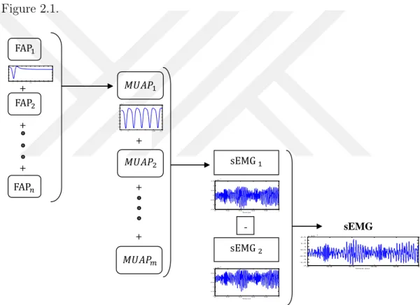
Main components of the model is shown in the diagram which is represented in Figure 2.1. + + + + - sEMG 00.010.020.030.040.050.060.070.080.090.1 -20 -15 -10 -5 0 5 x 10⁻⁶ Time (s) 0 0.02 0.04 0.06 0.08 0.1 -4 -3 -2 -1 0 1 2 x 10⁻⁵ Time (s) 0 0.2 0.4 0.6 0.8 1 -1.5 -1 -0.5 0 0.5 1 1.5x 10⁻⁴ Time (s) + + 0 0.2 0.4 0.6 0.8 1 -2 -1.5 -1 -0.5 0 0.5 1x 10⁻⁴ Time (s) 0 0.2 0.4 0.6 0.8 1 -2 -1.5 -1 -0.5 0 0.5 1 1.5 2 2.5x 10⁻⁴ Time (s )
Figure 2.1: Architecture of the sEMG model. Basic operations of generating a sEMG signal that simulate the signals obtained from one channel are shown in the figure. Signal graphs show 1 second signal simulations (FAP: Fiber Action Potential, MUAP: Motor Unit Action Potential, SEMG: Surface EMG).
The diagram shows the main operations of the constructed model to generate the sEMG signal. Basically, superposition of several fiber action potentials con-stitute a motor unit action potential (e.g. MUAP1) as illustrated in Figure 2.1. Other MUAPs which involve the constitution of sEMG1 signal are created by contribution of different number of fibers for each MUAP. sEM G1 and sEM G2
order to simulate bipolar electrode configuration recordings, signals of these two electrodes are subtracted from each other to form the resultant signal sEM G.
2.2.1.4 Fiber action potential in intracellular field
Simulation of a sEMG signal starts from the intracellular level. As it is mentioned previously, a single fiber action potential initiate at the NMJ of the fiber where the activation command received. Generated action potentials at the NMJ (locates in the middle of the fiber approximately) of a fiber propagate along the fiber length towards two opposite directions longitudinally with a constant velocity and extinguish at the tendon ends of the fiber [66]. This propagation mechanism is attempted to simulate in the current model. It is assumed that potential has triphasic shape. Three poles are calculated symmetrically located both side of the NMJ which is denoted as z within this manner using current distribution equation 2.2 which is derived from the fiber action potential equation 2.1. Consequently 6 poles are obtained for each instant current positions, 3 poles of each action potential propagate along the fiber length by the equation cvt in time t in opposite
directions.
Intracellular action potential of a fiber is denoted by the mathematical expres-sion:
Vm(z) = A(Λz)3e−Λz− B. (2.1)
and second derivative of the fiber potential is the current distribution [52] which is calculated as:
Im = CAΛ2(Λz)[6 − 6Λz + (Λz)2]e−Λz (2.2)
conduction velocity and time, calculated as cvt. A and B are action and resting
state potential constants respectively.
2.2.1.5 Fiber action potential in extracellular field
Tissue between the source (active fiber cell NMJ point inside the muscle) and the skin affects the signal recorded over the skin. For the sake of simplicity, tissue effects such as low pass filtering are neglected in the model. It is not aimed to create a realistic model in the present study as it is mentioned previously.
Since a sEMG model is indented to generate, calculated potentials in the in-tracellular level are transformed to the skin level. Thus, action potential of a fiber that is detected over the surface of the skin is formulated in the model as:
V = 1 2πσr X Pi q (h2)K a+ (zi− z)2 (2.3)
σr is electric conductivity (S/mm) along fiber radius r, Pi is current value of
the pole i that is calculated using equation 2.2, h is depth of the fiber underneath the skin, Ka is anisotropy ratio(ratio between conductivities in the longitudinal
and perpendicular directions) that equals to σz/σr, σz and σr are electric
con-ductivities along z and r directions, Zi is distance between electrode location and
the NMJ along fiber length parallel to the skin surface.
2.2.1.6 Motor unit action potential
As it is mentioned previously, a MUAP is the superposition of fiber action po-tentials which are involved in the electrode detection field. Different number of fibers are defined and MUAPs that is generated on the surface of the skin are calculated using the equation 2.3 for each MU. MUAP shape and the amplitude highly depends on the factors like distance between detection site and origin of the signal [61], number of fibers and their firing rates and conduction velocity etc.
These effects are clearly observed during simulation calculations. For instance, there is an inverse relationship between the duration time of an action poten-tial and its conduction velocity, as it has been revealed in De Lucas study [67]. Thus, same conduction velocities (cv) are determined for each fiber of a MU but
conduction velocity for each MU is different.
2.2.1.7 Surface EMG signal simulation
After calculating a single MUAP, there were three more steps that should be taken to achieve the intended model solution. These steps can be listed as: electrode signal simulation, bipolar recording simulation and final sEMG signal simulation. Resulted sEMG signal represents the signal which is recorded from one channel. Movement simulations have been made accordingly by changing the parameters (e.g. firing rate, number of fibers, and conduction velocity of the fiber) of the involved fibers for each channel.
A duration time was determined for the signal simulations (20 seconds signals are generated). MUAPs are generated repeatedly by varying firing rates. Firing rate of the MUAPs was reduced by two (2) for the following MUAPs that will be involved into the signal that is recorded from one electrode. This process simply constitutes MUAP train (MUAPT) in the predetermined time interval. Number of occurrences of one MUAP in the MUAPT varies according to the firing rate, electrode-source distance and time interval. Additionally, electrode location values of the fibers are increased incrementally to simulate action potentials move in time (generating times of the single fiber action potentials differ), simply to generate MUAPTs. Consequently, linear summation of the MUAPTs constitutes the sEMG signal which is recorded from one of the electrodes in the bipolar electrode pair [52].
Only difference between the bipolar electrode signals is having different za
(electrode position) values, all the other parameters are exactly same for each sEMGs (these are sEMG1 and sEMG2 signals as represented in Figure 2.1).
electrode pairs was 2 cm approximately and same for all movement simulations. It can be considered as second electrode recordings are different representation of the first electrode signals shifted in time. However they are not exactly same, due to different initial electrode locations resultant signal vary in time (differ in shape and amplitude).
To simulate different movements, the parameters like number of MUs, number of fibers of each MU and the conduction velocities of the fibers for each MU are adjusted differently for each channel. These parameter adjustments enable the simulation of distinct movement signals in terms of shape and amplitude for each channel signals. [68]
2.2.1.8 Assumptions of the model
The action potential of a fiber is generated as a tripole. It is assumed that fibers of the motor units are distributed parallel to the skin. All the fibers are assumed to be in the same depth and have same length and radius. The diameters of the fibers are neglected. Fibers are considered as line sources. The difference between firing rate of the MUs and the distance between two bipolar electrodes were same for each generated sEMG signal. Electrode spatial extent is restricted only to parallel direction to the skin, along to fiber length. Tissue effect between the electrode and the source is neglected. Different conduction velocities, number of MUs and fibers of each MU are determined to constitute different sEMG signals in terms of shape and amplitude.
2.2.2
Distorted Signal Simulation
Amplitudes of the simulated signals are changed gradually (increased and de-creased) to create distortions like in the conditions sweating or misconduct issues between skin and the electrode. Loose conduct between the skin and the elec-trodes may lead to decrease and sweating may lead to increase on the amplitude of the EMG signals. Classification and adaptation performances are investigated
during variations of the signal.
Different amount of distortion levels have been applied to all of the previously simulated movement signals. Distorted signal patterns are created for each simu-lated movement signal. Distortion only applied to the signals of the one channel of the channel pair.
Distorted signals are simulated as amplitude changes on the signals using the equation[69]:
y = (1 ± d)y (2.4)
where y is the signal which is intended to distort, d is the rate of distortion. − and + signs are for the adjustment of the distortion level. − decrease and + increase the amplitude of the signal y.
2.2.3
Neural Network Adaptation
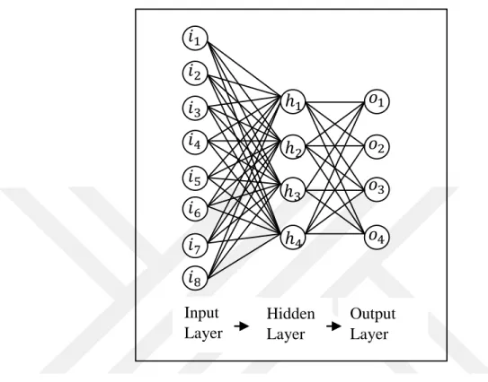
General architecture of the system is shown in Figure 2.3. An adaptive neural network classification algorithm is developed to adapt to the variations in the signals. Training and test data sets are constructed by extracting features from the simulated signals. A simple three layered feed-forward neural network used as the main classifier that calculate initial outputs. Neural network that is used in the present study is consisted of 8 input, 4 hidden, 4 output layer neurons. Structure of the network is illustrated in Figure 2.2.
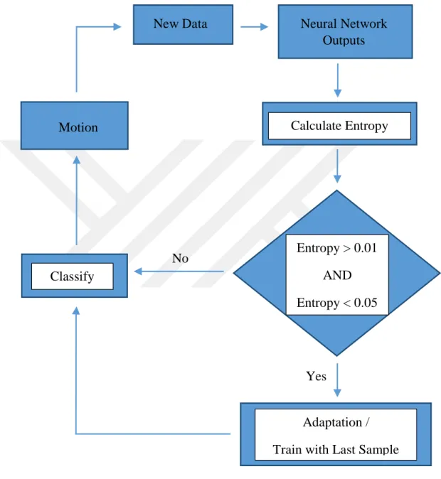
Calculated outputs are not accepted as classifier decisions directly. An eval-uative confidence metric, entropy, is used to control classifier outputs. Entropy can be calculated using Equation 3.1(in Chapter 3). Interpretations that made by entropy calculation basically based on the argument; high entropy means low confidence and low entropy means high confidence. Entropy thresholds are
deter-Input Layer Hidden Layer Output Layer
Figure 2.2: Structure of the neural network.
where adaptation can be applicable. It is assumed that entropy increases but no wrong classifications occur in these threshold intervals. Thresholds are defined empirically after several evaluations made on the classification results. Simulta-neous classifier decision results and entropy calculation plots made easier to spot increased but correctly classified entropy values. Thus, entropy value of the net-work output is controlled immediately to check the difference between calculated entropy and the threshold intervals. If the calculated entropy value fits in the threshold intervals classifier is retrained by this recent input samples, otherwise classifier makes the decision without any retraining process (retraining was held by applying back propagation online learning and only the last sample used to update network weights that can be used for the next classifications). This is the first version of our adaptive neural network, details about the classifier will be given and expanded version of the classifier will be introduced in the next chapter (Chapter 3).
Yes New Data Entropy > 0.01 AND Entropy < 0.05 Calculate Entropy Adaptation / Train with Last Sample No
Classify Motion
Neural Network Outputs
2.3
Results
2.3.1
Simulated Signals
20 seconds signals are simulated for each movement. Constant parameters were determined as: A = 96mV is action potential, B = 90mV resting state potential and radial conductivity; σr =0,330 [60].
2.3.1.1 Wrist extension movement simulation
Wrist extension movement signal simulation is plotted in Figure 2.4.
0 2 4 6 8 10 12 14 16 18 20 −1 −0.5 0 0.5 1x 10 −3 Channel 1 Time(s) 0 2 4 6 8 10 12 14 16 18 20 −1 −0.5 0 0.5 1x 10 −3 Channel 2 Time(s)
Figure 2.4: Simulated signal of movement wrist extension. Parameters of the simulated signal wrist extension:
Channel 1:
Conduction velocities of each MU respectively = [6 6.5 7 7 7.2 7.5 7.5 8 8 8 8]m/s. Number of fiber of each MU = 10.
Channel 2:
Conduction velocities of each MU respectively = [4 4.4 5 5 5.5 5.5]m/s. Number of fiber of each MU = 5.
2.3.1.2 Wrist flexion movement simulation
Wrist flexion movement signal simulation is plotted in Figure 2.5.
0 2 4 6 8 10 12 14 16 18 20 −1 −0.5 0 0.5 1x 10 −3 Channel 1 Time(s) 0 2 4 6 8 10 12 14 16 18 20 −1 −0.5 0 0.5 1x 10 −3 Channel 2 Time(s)
Figure 2.5: Simulated signal of movement wrist flexion.
Parameters of the simulated signal wrist flexion: Channel 1:
Conduction velocities of each MU respectively = [4 4 4 5 5 5.5]m/s. Number of fiber of each MU = 5.
Channel 2:
Conduction velocities of each MU respectively = [6.5 6.5 6.5 6.5 7 7 7 7.2 8 8 8]m/s. Number of fiber of each MU = 10.
2.3.1.3 Hand close movement simulation
Hand close movement signal simulation is plotted in Figure 2.6. Parameters of the simulated signal hand close:
Channel 1:
Conduction velocities of each MU respectively = [4 4 5 5 5.5 6 7 7.2 7.5 8 8 8]m/s. Number of fiber of each MU = 10.
0 2 4 6 8 10 12 14 16 18 20 −1 −0.5 0 0.5 1x 10 −3 Channel 1 Time(s) 0 2 4 6 8 10 12 14 16 18 20 −1 −0.5 0 0.5 1x 10 −3 Channel 2 Time(s)
Figure 2.6: Simulated signal of movement hand close.
Conduction velocities of each MU respectively = [4 4.4 5 5 5.5 5.5 6.5 6.5 7 8 8]m/s. Number of fiber of each MU = 10.
2.3.1.4 Hand open movement simulation
Hand open movement signal simulation is plotted in Figure 2.7.
0 2 4 6 8 10 12 14 16 18 20 −1 −0.5 0 0.5 1x 10 −3 Channel 1 Time(s) 0 2 4 6 8 10 12 14 16 18 20 −1 −0.5 0 0.5 1x 10 −3 Channel 2 Time(s)
Figure 2.7: Simulated signal of movement hand open.
Parameters of the simulated signal hand open: Channel 1:
Conduction velocities of each MU respectively = [4 4 5 5 6 7 7 7.2 7.5 8 8]m/s. Number of fiber of each MU = 10.
Channel 2:
Conduction velocities of each MU respectively = [4 5 5 5.5 5.5 6 6]m/s. Number of fiber of each MU = 7.
2.3.2
Adaptation Results for Distorted Signals
2.3.2.1 Distorted signals
First 10 seconds of the simulated 20-seconds sEMG signal is distorted in differ-ent levels and appended consecutively to create three differdiffer-ent distorted signal arrangements (DT1-3). 10 seconds of the signal corresponds to 200 samples of the simulated patterns. Distortion is applied only on the signals corresponding to the first channel in each movement.
Three different signal arrangements (DT1-3) are made for each movement sig-nal pattern. Distortion arrangement types are described below for each differently arranged signal patterns:
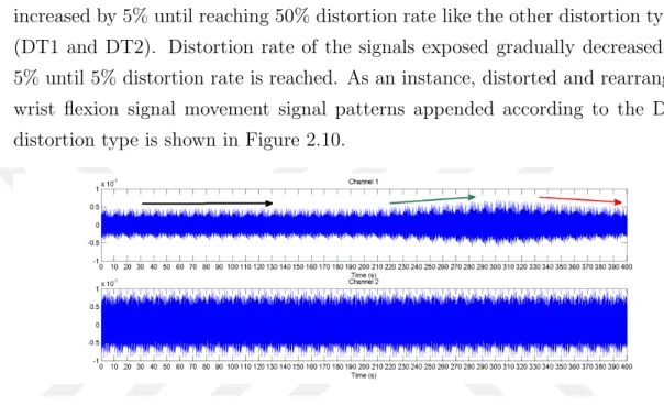
Distortion type 1 (DT1): Starting with 10 seconds of the simulated undis-torted signal patterns, 5% distortion rate is applied to the same undisundis-torted signal and appended at end of the undistorted signal. This process is continued incrementing distortion rate by 5% until distortion rate reaches 50%. After that, distortion rate that is applied on the simulated signal start to decrease by 5% until reaching 0% distortion rate -it will be the same undistorted signal that was given to the neural network at the beginning. The same undistorted 10 seconds signal patterns are appended to at the end of the signal arrangement (DT1) three times. As an instance, distorted and rearranged wrist flexion movement signal patterns appended according to the DT1 distortion type is shown in Figure 2.8.
0 10 20 30 40 50 60 70 80 90 100 110 120 130 140 150 160 170 180 190 200 210 220 230 240 −1 −0.5 0 0.5 1x 10 −3 Channel 1 Time (s) 0 10 20 30 40 50 60 70 80 90 100 110 120 130 140 150 160 170 180 190 200 210 220 230 240 −1 −0.5 0 0.5 1x 10 −3 Channel 2 Time (s)
Figure 2.8: Distorted wrist flexion movement signal which is arranged by DT1 same 10 seconds undistorted signal exposed starts to increase by 5%. Increasing distortion rate is continued until distortion rate reaches 50%. It is the maximum level of the distortion, after that distortion rate start to decrease gradually by 5% until reaching 0% distortion rate. Each distorted signal is appended next to each other. 10 seconds undistorted signal patterns are added at the end of the distorted signals several times (i.e. 20 times). As an instance, distorted and rearranged wrist flexion movement signal patterns appended according to the DT2 distortion type is shown in Figure 2.9.
0 10 20 30 40 50 60 70 80 90 100 110 120 130 140 150 160 170 180 190 200 210 220 230 240 250 260 270 280 290 300 310 320 330 340 350 360 370 380 390 400 −1 −0.5 0 0.5 1x 10 −3 Channel 1 Time (s) 0 10 20 30 40 50 60 70 80 90 100 110 120 130 140 150 160 170 180 190 200 210 220 230 240 250 260 270 280 290 300 310 320 330 340 350 360 370 380 390 400 −1 −0.5 0 0.5 1x 10 −3 Channel 2 Time (s)
Figure 2.9: Distorted wrist flexion movement signal which is arranged by DT2 Distortion type 3 (DT3): Undistorted 10 seconds signals are appended at
the beginning of the signal arrangement 20 times. Afterwards, the undistorted signals start to distort by 5% distortion rate. Distortion rate is incrementally increased by 5% until reaching 50% distortion rate like the other distortion types (DT1 and DT2). Distortion rate of the signals exposed gradually decreased by 5% until 5% distortion rate is reached. As an instance, distorted and rearranged wrist flexion signal movement signal patterns appended according to the DT3 distortion type is shown in Figure 2.10.
Figure 2.10: Distorted wrist flexion movement signal which is arranged by DT3
2.3.2.2 Adaptive neural network
Neural network that is used in the present study is consisted from 8 input, 4 hidden and 4 output layer neurons as it is mentioned in the methods section. Learning rate that is used during training of the classifier to obtain initial weights and during adaptation process was same (i.e. 0.15). Training of the constructed neural network is continued until all movement patterns are correctly classified (after 16374 epochs training stopped). Training and test data are constructed by extracting root mean square (RMS) and wavelength (WL) features separately from all time windows of simulated signals. Movement data patterns (extracted feature vectors from time windows) are fed to the neural network in the following order: wrist flexion, hand close, wrist extension and hand open. Upper entropy threshold is 0.05 and lower threshold is 0.01. Adaptation is applied when the entropy that is calculated from the decision outputs is in this threshold interval
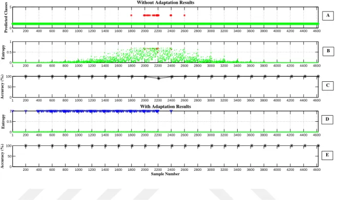
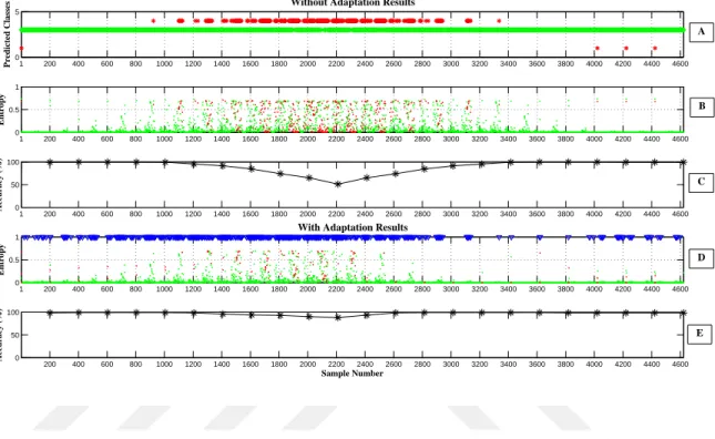
Classification accuracy results for each distortion type (DT1-DT3) and for each movement are shown in Figures 2.11, 2.12, 2.13, 2.14. The results of the movement signal patterns are represented in the same order as the movement patterns are fed to the neural network. Every 10 seconds, the signal classification accuracy is calculated using Equation 3.3 and shown below in graphs.
Results for DT1:
The results for DT1 signal classification are shown in the graphs for each movement with the same order as the movement patterns were fed to the classifier. Figures 2.11, 2.12, 2.13, 2.14 present wrist flexion, hand close, wrist extension and hand open movements classification accuracy results, respectively.
Results for DT2:
The results for DT2 signal classification are shown in the graphs for each movement with the same order as the movement patterns were fed to the classifier. Figure 2.15 presents wrist flexion results, 2.16 presents hand close results, 2.17 presents wrist extension results, 2.18 presents hand open results, respectively.
Results for DT3:
The results for DT3 signal classification are shown in the graphs for each movement with the same order as the movement patterns were fed to the classifier. Figure 2.19 presents wrist flexion results, 2.20 presents hand close results, 2.21 presents wrist extension results, 2.22 presents hand open results, respectively.
1 200 400 600 800 1000 1200 1400 1600 1800 2000 2200 2400 2600 2800 3000 3200 3400 3600 3800 4000 4200 4400 4600 0
5
Without Adaptation Results
Predicted Classes 1 200 400 600 800 1000 1200 1400 1600 1800 2000 2200 2400 2600 2800 3000 3200 3400 3600 3800 4000 4200 4400 4600 0 0.5 1 Entropy 1 200 400 600 800 1000 1200 1400 1600 1800 2000 2200 2400 2600 2800 3000 3200 3400 3600 3800 4000 4200 4400 4600 0 50 100 Accuracy (%) 1 200 400 600 800 1000 1200 1400 1600 1800 2000 2200 2400 2600 2800 3000 3200 3400 3600 3800 4000 4200 4400 4600 0 0.5 1 Entropy
With Adaptation Results
200 400 600 800 1000 1200 1400 1600 1800 2000 2200 2400 2600 2800 3000 3200 3400 3600 3800 4000 4200 4400 4600 0 50 100 Accuracy (%) Sample Number D C B A E
Figure 2.11: The classification accuracy results for type 1 distorted (DT1) for wrist flexion movement. The classification results where no adaptation is applied are shown in graphs A, B and C. A) The output class labels of the network for each data point(sample). Class labels are represented by numbers 1 to 4 for wrist flexion, wrist extension, hand close, hand open movements, respectively. Green stars and red stars represent true and wrong classified samples by the classifier, respectively. B) Entropy after each decision of the classifier. C) Classification accuracy calculations shown by black stars for every 200 samples.
Classification results where adaptation is applied are shown in graphs D & E. D) Entropy after each classification (adaptation is applied during classification). E) Classification accuracy calculations for every 200 samples shown by black stars. The samples where the adaptation applied marked by blue vertical triangles.
2.4
Discussion
Wrist flexion movement patterns are the first patterns that are fed to the network. The classification accuracy results for type 1 distorted signals for the movement are shown in Figure 2.11. The highest distortion level corresponds to the samples where the highest entropy values are observed (Figure 2.11B). Meanwhile, the patterns where the lowest accuracies (Figure 2.11C) are observed have the highest entropy value (Figure 2.11B). The increase and the decrease in the entropy trends can be clearly seen from Figure 2.11B. When the entropy graphs are compared for the cases in which adaptation is applied (Figure 2.11D) and not applied (Figure 2.11B), it can be said that after applying adaptation, entropy is substantially decreased as expected. As a result of decrease in the entropy, increases are observed in the classification accuracies (Figure 2.11D).
No decrease is observed in the classification accuracy for the next upcoming patterns (hand close movement patterns), when the accuracy results of the first samples of the movement in the cases where adaptation is applied and not applied are compared which are shown in Figure 2.12C and E. It shows that previously applied adaptations (in the wrist flexion movement patterns) did not lead to any difference on the classification accuracy. Nevertheless, adaptation points are seen at the first samples of the movement due to the increased entropy. The number of adaptation points are gradually increased for the next samples of the movement as a result of the gradual distortion increases. When adaptation is not applied, accuracy starts to decrease after 1000 samples, it corresponds to the samples where 25% distortion rate is applied, decrease continues until reaching 50% dis-tortion rate, lowest accuracy is observed as a result of 50% disdis-tortion in Figure 2.12B. In addition, in the classification accuracy results where the adaptation applied (Figure 2.12E), starting from the samples where classification accuracy start to decrease (25% distortion rate) in the case of no adaptation applied (Fig-ure 2.12C), it is observed that adaptation algorithm starts to recover distortion effects on the accuracy. It is valid even for the cases where highest distortion rate is reached, significant enhancement on the accuracy can be seen in Figure 2.12E when it is compared with the accuracy results where no adaptation applied (Figure 2.12C). Since it is the second time of the algorithm comes across with