Massively parallel mapping of next generation sequence reads using GPU

MASSIVELY PARALLEL MAPPING OF

NEXT GENERATION SEQUENCE READS

USING GPU

a thesis

submitted to the department of computer engineering

and the graduate school of engineering and science

of bilkent university

in partial fulfillment of the requirements

for the degree of

master of science

By

Mustafa Korkmaz

November, 2012

I certify that I have read this thesis and that in my opinion it is fully adequate, in scope and in quality, as a thesis for the degree of Master of Science.

Prof. Dr. Cevdet Aykanat (Advisor)

I certify that I have read this thesis and that in my opinion it is fully adequate, in scope and in quality, as a thesis for the degree of Master of Science.

Assist. Prof. Dr. Can Alkan (Co-Advisor)

I certify that I have read this thesis and that in my opinion it is fully adequate, in scope and in quality, as a thesis for the degree of Master of Science.

Assoc. Prof. Dr. Hakan Ferhatosmano˘glu

I certify that I have read this thesis and that in my opinion it is fully adequate, in scope and in quality, as a thesis for the degree of Master of Science.

Assoc. Prof. Dr. O˘guz Ergin

Approved for the Graduate School of Engineering and Science:

Prof. Dr. Levent Onural Director of the Graduate School

ABSTRACT

MASSIVELY PARALLEL MAPPING OF NEXT

GENERATION SEQUENCE READS USING GPU

Mustafa Korkmaz M.S. in Computer Engineering

Supervisors: Prof. Dr. Cevdet Aykanat and Assist. Prof. Dr. Can Alkan November, 2012

The high throughput sequencing (HTS) methods have already started to funda-mentally revolutionize the area of genome research through low-cost and high-throughput genome sequencing. However, the sheer size of data imposes various computational challenges. For example, in the Illumina HiSeq2000, each run pro-duces over 7-8 billion short reads and over 600 Gb of base pairs of sequence data within less than 10 days. For most applications, analysis of HTS data starts with read mapping, i.e. finding the locations of these short sequence reads in a reference genome assembly.

The similarities between two sequences can be determined by computing their optimal global alignments using a dynamic programming method called the Needleman-Wunsch algorithm. The Needleman-Wunsch algorithm is widely used in hash-based DNA read mapping algorithms because of its guaranteed sensitivity. However, the quadratic time complexity of this algorithm makes it highly time-consuming and the main bottleneck in analysis. In addition to this drawback, the short length of reads ( ∼100 base pairs) and the large size of mammalian genomes (3.1 Gbp for human) worsens the situation by requiring several hundreds to tens of thousands of Needleman-Wunsch calculations per read. The fastest approach proposed so far avoids Needleman-Wunsch and maps the data described above in 70 CPU days with lower sensitivity. More sensitive mapping approaches are even slower. We propose that efficient parallel implementations of string comparison will dramatically improve the running time of this process. With this motivation, we propose to develop enhanced algorithms to exploit the parallel architecture of GPUs.

¨

OZET

YEN˙I NES˙IL D˙IZ˙ILEME B ¨

OL ¨

UTLER˙IN˙IN GRAF˙IK

˙IS¸LEME B˙IR˙IM˙I KULLANILARAK YO ˘

GUN PARALEL

ES

¸LENMES˙I

Mustafa Korkmaz

Bilgisayar M¨uhendisli˘gi, Y¨uksek Lisans

Tez Y¨oneticileri: Prof. Dr. Cevdet Aykanat ve Yrd. Do¸c. Dr. Can Alkan Kasım, 2012

Y¨uksek ¸cıktılı dizileme (YC¸ D) y¨ontemleri, d¨u¸s¨uk maliyeti ve y¨uksek ¸cıktı ver-mesiyle, daha ¸simdiden genom ara¸stırmaları alanında temelden bir devrim ger¸cekle¸stirdi. Ancak, elde edilen verinin b¨uy¨uk olması, ¸ce¸sitli hesaplama ta-banlı sorunları da beraberinde getirdi. ¨Orne˘gin, Illumina HiSeq2000 modelinde, her bir ¸calı¸sma sonrası, 7-8 milyardan fazla k¨u¸c¨uk DNA b¨ol¨ut¨u ve 600 Gb dan fazla baz ¸cifti 10 g¨un i¸cinde elde edilebilmektedr. Bir¸cok uygulama i¸cin, YC¸ D verilerinin ¸c¨oz¨umlenmesi k¨u¸c¨uk DNA b¨ol¨utlerinin e¸slenmesiyle ba¸slar. ¨Orne˘gin, k¨u¸c¨uk DNA par¸calarının kaynak DNA’daki yerlerinin tespit edilmesi gibi.

˙Iki dizinin arasındaki benzerlik, en uygun genel hizalamalarının Needleman-Wunsch algoritması yarımıyla hesaplanmasıyla bulunur. Needleman-Wunsch algoritması y¨uksek duyarlılı˘gı sebebiyle, karma tablo tabanlı k¨u¸c¨uk DNA b¨ol¨utlerinin e¸slenmesi algoritmalarında kullanılır. Ancak bu algoritmanın ik-ilenik karma¸sıklıktaki yapısı, fazla zaman harcamasına ve analizlerde darbo˘gaz olu¸sturmasına sebep olur. Bu engelin yanında DNA b¨ol¨utlerinin k¨u¸c¨ukl¨u˘g¨u (yakla¸sık 100 baz ¸cifti) ve memeli genomlarının b¨uy¨ukl¨u˘g¨u (3.1 Giga baz ¸cifti), her bir k¨u¸c¨uk DNA b¨ol¨ut¨u i¸cin y¨uzlerce ila onbinlerce arası hesaplama yapılmasını gerektirerek, durmu daha da k¨ot¨u hale getirmektedir. Needleman-Wunsch algo-ritmasını kullanmadan ¸calı¸san ve yukarıdaki veriyi kullanan en hızlı uygulama 70 M˙IB g¨un¨unde, az duyarlılıkta ¸calı¸smaktadır. Daha duyarlı olan yakla¸sımlar ise daha da yava¸s ¸calı¸smaktadır. Bu tezde, etkili bir paralel dizi kar¸sıla¸stırma yapısı geli¸stirirek, bu uygulamanın ba¸sarımını ciddi seviyelerde arttırıldı˘gını ¨onerdik. Bu g¨ud¨ulenmeyle yola ¸cıkarak, grafik i¸slem birimlerinin paralel mimarisinin kul-lanan geli¸smi¸s bir yakla¸sım ortaya koyduk.

Acknowledgement

I consider it an honour to be under the supervision of Prof. Dr. Cevdet Aykanat and Assist. Prof. Dr. Can Alkan. This thesis would not happen to be possible without their guidance and advices.

I am grateful to Assoc. Prof. Dr. Hakan Ferhatosmano˘glu and Assoc. Prof. Dr. O˘guz Ergin for reading and commenting on this thesis.

I would like to thank to my friends and colleagues for their fellowship, espe-cially Can, Enver, Seher, ˙Ilker, ¨Omer, S¸¨ukr¨u, Salim, Halil, Ata, Beng¨u, Gizem, K¨o¸sker, G¨okhan and ˙Ibrahim.

I owe my deepest gratitude to my parents M¨uberra and Nabi and especially my brother ¨Omer, for their understanding and supporting me throughout my life.

I would like to thank to the Scientific and Technological Research Council of Turkey (T ¨UB˙ITAK) for providing financial assistance during my study.

Finally, and most importantly, I would like to thank to my wife Zeynep for emotional support, understanding and love . . .

Contents

2.2 Whole Genome Sequencing . . . 8

2.3 Read Mapping . . . 9

2.4 Hash Based Seed & Extend . . . 11

2.5 Needleman-Wunsch Algorithm . . . 14

2.5.1 Initialization . . . 15

2.5.2 Alignment Matrix Calculation . . . 15

2.5.3 Backtracking . . . 17

CONTENTS vii

2.6.1 Thread Hierarchy . . . 21

2.6.2 Memory Hierarchy . . . 22

3 Related Work 25 4 A Parallel Alignment Scheme 28 4.1 Anti-diagonal Parallelism . . . 29

4.2 Ukkonen’s Edit Distance . . . 32

4.3 Parallel Alignment . . . 33

4.4 CUDA Optimizations . . . 38

5 Experimental Results 40 5.1 Environment and Implementation . . . 40

5.2 Experiments . . . 41

List of Figures

2.1 Double helix structure of DNA molecules [1]. . . 7

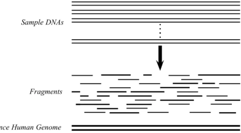
2.2 Example of Whole Genome Shotgun Sequencing process. From many sample genomes, millions of fragments are extracted. . . 9

2.3 Sequencing instruments output Kilobasepair (Kbp) per year [2]. . 10

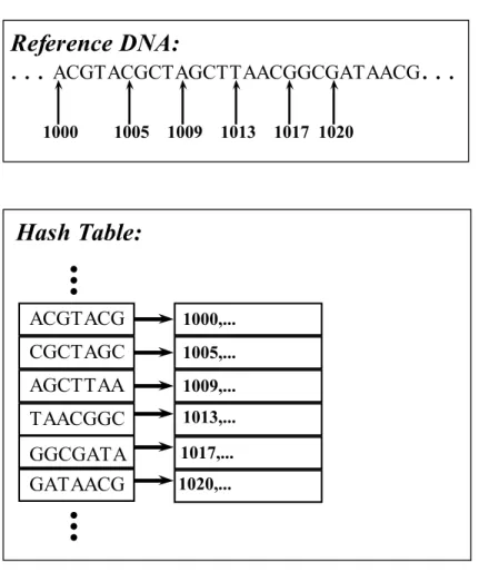
2.4 Portion of a sample hash table. Here are several reference genome fragments are stored as keys and their locations in reference DNA are stored as values. In this example, the fragments are 7 bp long. 12

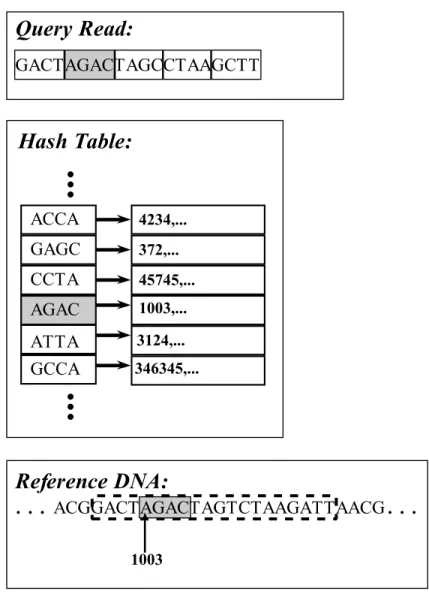
2.5 Choosing the right substring from the reference DNA. First, second gram of the query read is located in hash table. Corresponding 4-gram location is selected from reference DNA as well as its one left, three right neighbour 4-gram as it is the second 4-gram in query read.Notice that there can be some errors in neighbour 4-grams. . 13

2.6 An example comparison of global and semi-global alignment. Edit distance of global and semi-global alignment is −4. On the other hand, if we ignore the trailing gaps, semi-global alignment’s edit distance is 6, which is higher than global alignment score. . . 14

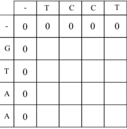
2.7 Initial alignment matrix of sequences “GTAA” and “TCCT”. No-tice that the first column and row are residual since corresponding sequence item is N U LL. . . 15

LIST OF FIGURES ix

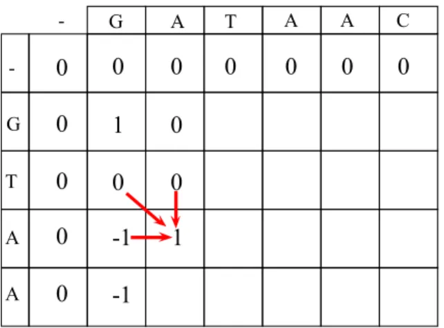
2.8 A sample alignment matrix calculation. . . 16

2.9 A sample backtracking over calculated alignment matrix. End gaps of read query are not penalized.Alignment is completed with an two indels. . . 18

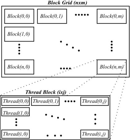
2.10 A sample thread structure kernel setup. The grid has n × m blocks in nxm 2D structure and a block has i×j threads in i×j 2D structure. 22

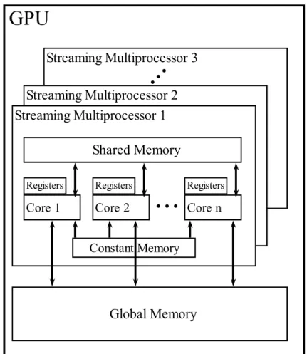
2.11 CUDA memory layout . . . 24

4.1 (a) Column by column order. and (b) row by row order. In both strategies, a cell is dependent to the previously computed cell in the corresponding order. (Darker cell is dependent to lighter cells) 30

4.2 Example of anti-diagonal order. The computation of block black cell depends on the values already computed and stored in the three grey cells. . . 31

4.3 Example of calculated cells according to Ukkonen’s edit distance algorithm. Number of indels t = 4 and only shaded cells are calcu-lated. The darker cells show the in main diagonals and the lighter cells are neighbour diagonals. . . 33

4.4 An order for multiple matrix per thread block. Each matrix data is stored in anti-diagonal order alongside. . . 35

4.5 Interleaved anti-diagonal memory layout. . . 36

4.6 Change in padding strategy. Notice that the bottom-right triangle cell group of area of calculations has no padded data and the first row and column is padded with 0 as semi-global alignment requires. 37

4.7 An example multiple matrix setup according to IML. The data is stored in anti-diagonal order. In each iteration, corresponding cells are calculated by threads concurrently except the pads. . . 38

LIST OF FIGURES x

5.1 The comparison between two different GPU implementations. (Read Size:100, Reference DNA Segment Size:106, Tolerated In-del:3) . . . 42

5.2 The comparison between two different GPU implementations in various number of threads per block (Read Size:100, Reference DNA Segment Size:106, Tolerated Indel:3). . . 43

5.3 The comparison between two different GPU implementations in various sizes of reads and reference DNA segments. . . 44

5.4 The comparison between CPU and BML implementation in various number of matrices. (Read Size:100, Reference Size:106, Tolerated Indel:3) . . . 45

5.5 The comparison between IML and CPU implementations in vari-ous sizes of reads and reference DNA segments. . . 46

List of Tables

5.1 IML speed-up over BML (Read Size:100, Reference DNA Segment Size:106, Tolerated Indel:3). . . 42

5.2 IML speed-up over CPU. (Read Size:100, Reference DNA Segment Size:106, Tolerated Indel:3) . . . 45

Chapter 1

Introduction

One of the major purposes of bioinformatics is to process data obtained from molecular biology experiments and obtain meaningful results [3]. Exploring protein and gene structure is the most important problem in bioinformatics. Especially sequence analysis is a very important since all protein, DNA, and RNA sequences contain significant information needed for their functions. DNA molecules are responsible for holding the information of how cell works. RNAs transport short pieces of information and work as a template for protein synthe-sis. And lastly, proteins are mainly one of the building blocks of livings, and also form enzymes.

Sequencing is attracting more and more interest thanks to the recent advances in technology. It gives us unprecedented power to explore and reveal almost all information about organisms. DNA sequencing is a valuable information source for disciplines like genetics, medical genomics, and many others. It helps uncover the population migrations and relations and delineates the evolution of a species. Naturally, humans are the most studied species by the data provided from se-quencing. Diagnosis of diseases can be done more accurately. Predispositions to diseases can be detected earlier. Additionally, a new experimental treatment method called gene therapy aims to replace defective genes with normal ones. Besides, drug efficacy is increased by using DNA information and custom drugs are produced for certain diseases. DNA forensics is another important tool that

is used in identifying suspects and establishing relations with family members. In addition, knowledge on DNA also affected agriculture and animal husbandry. Healthier and more productive animals are bred and more nutritious and resis-tant crops are produced. There are more potential benefits, which will put in practice by obtaining more and more information from sequences. Among these macro-molecules, DNA sequence analysis attracts the most attention since the DNA contains the most basic information. Depending on the species, its genome contains hundreds of thousands to billions of atomic information.

To obtain the information of a DNA molecule from a sample, first a process called shotgun sequencing is applied that yields some smaller DNA segments with no information about their original place in the complete DNA sequence . Then, these small parts are assembled with the help of sophisticated algorithms. The number of small segments is large and size of a single segment is short. There are two different main approaches for sequence processing. The first one is called resequencing, which involves comparing short sequence segments to an existing reference, and the second one is de novo assembly, which involves assembling short segments with no reference. In this thesis, we focus on improving the performance of the DNA resequencing analysis.

1.1

Motivation

DNA resequencing is defined as comparing DNA map of an organism with a reference genome. Quantity and quality of the output of the sequencing phase give direction to the researches. Whole Genome Shotgun sequencing (WGS) [4] is commonly used for obtaining the DNA information of a sample. WGS approach basically extracts the DNA from sample as small fragments, and the prefix and suffixes are read, in different sizes that follows some interval size distribution. After the WGS process, short reads are ordered and mapped to a reference DNA. There are two main paradigms for read mapping. The first one is Burrows -Wheeler Transform (BWT) [5] and Ferragini-Manzini Index(FM) [6] aligning and the second one is hash based seed and extend method [7]. The first approach is

based on a well-known data compression method where genome is transformed and indexed. The approach runs fast for perfect matches however imperfect hits dramatically reduces the performance. In the second approach, reference DNA is divided into segments and stored in a hash table which queries are aligned to the values obtained from. This type of algorithms requires large memory and they are slower than Burrows-Wheeler approach. On the other hand, the approach is error-tolerant.

The two main problems in mapping is first, to deal large data and second, the data is not perfect, there are errors caused by sequencing instruments and real variation in sample DNA. Thus, a good mapping algorithm needs to tolerate errors and must be fast. Mapping the data generated from the DNA of a sin-gle sample takes tens of CPU days. Throughput of DNA sequence machines are growing rapidly and getting cheaper with the advancements in sequencing tech-nologies and the data that needed to be deal is increasing faster than Moore’s Law [8]. Considering error-tolerance, scalability with respect to read length and relatively less random memory access, we decided to improve the performance of hash based seed and extend method.

The hash based seed and extend method can be examined as two parts. The first part is creating and managing the hash table and the second part is aligning DNA fragments. Alignment part is basically done by using a string comparison algorithm that utilize dynamic programming. Specific to sequencing by synthe-sis platforms such as Illumina, semi-global alignment works best, and we used Needleman-Wunsch algorithm for string comparison. Since the most time con-suming part of the algorithm is alignment part, it is very crucial to gain speedup in. For this, we used general purpose graphics processing unit (GPGPU) for ac-celeration. We calculated thousands of alignments in a parallel fashion and we used NVIDIA’s CUDA (Compute Unified Device Architecture) as our parallel system.

Processing hundreds of gigabytes of data is even more critical in terms of time complexity. For certain algorithms, comparison of subsequences are handled by using global alignment algorithm called Needleman-Wunsch. Although a single

alignment is not time-consuming, there are billions of comparisons executed for mapping data from single sample. In our work, we propose a parallel, fast memory aware Needleman-Wunsch algorithm model for graphics processing unit’s(GPU).

1.2

Contribution

The first contribution of this thesis is to map a time-consuming application to a commodity parallel GPU architecture. By this parallelism, we gain significant speed-up that will dramatically decrease the running time of DNA sequence anal-ysis. Read mapping is widely used in genomic mapping and alignment is usually handled with sequential programs or multi-threaded applications that follows an embarrassingly parallel paradigm. Thus, this real-life application will yield re-sults in reasonable time. Second, the program is easy to be merged with the existing and future hash table based resequencing applications. The program in-puts read and reference DNA segments arrays and outin-puts the alignment results. GPU as a general purpose parallelism, is cheap hardware so that the applica-tion can be used in cost effective computers. Finally, the applicaapplica-tion can run in various configurations like different read sizes, reference DNA segments size and error allowance .This provides a high flexibility of processing the outputs of different sequencing instruments since each generates various read sizes and error probability and are applicable to restricted applications like the ones only pro-cesses the different same-sized reads as well as the future works that will process relatively longer reads. Additionally, GPU thread and memory arguments are dynamically set for the best performance so that the application will work as an easy-to-integrate module without any configurations.

1.3

Outline

The outline of the thesis is follows: In Chapter 2, we give a short background on DNA sequencing and we describe related algorithms used in bioinformatics. In

Chapter 3, we briefly discuss previously proposed works that address the same problem. In Chapter 4, we explained the work we propose in this thesis in details. In Chapter 5, experimental results are demonstrated and described. At last, in Chapter 6, we conclude the thesis with a brief explanation of the contribution and future work.

Chapter 2

Background

Bioinformatics is merger of two main disciplines: Biological Sciences and Com-puter Science. Although the presented work is based on bioinformatic algorithms and a detailed knowledge on molecular biology is not necessary, a brief infor-mation about genetics, especially about DNA, RNA and protein sequences, is warranted for covering the background of the presented work.

2.1

Molecular Biology

Living organisms are consisted of organic compounds such as proteins, lipids and, carbon-hydrates. Among them, proteins are the most complex ones, since they form all the structures that perform vital operations. They form responsible for carrying out almost all the functions and they are the major components of the body structure. Some protein types are responsible for movement by muscle con-traction as well as defending body against antigens and carrying oxygen. There are many other duties that proteins get involved. What makes a protein molecule different from another is its structure that is dictated by its sequence. Proteins consist of amino acids. There are 20 protein builder amino acid molecules and they are combined in different sequences and they fold into 3-D structure to form different proteins. What decides the order of a sequence of amino acids is the

information stored in DNA molecules. DNA molecules are macromolecules that contain genetic information for all livings including protein synthesis.

A DNA (Deoxyribonucleic acid) molecule is a compound of repeating units called nucleotides. Nucleotides are bound as pairs and structured as two heli-cal chains. There are four different nucleotides: adenine, guanine, cytosine and thymine and they are abbreviated as A, G, C and T respectively. These nu-cleotides are linked as three hydrogen bonds between guanine and cytosine, and two hydrogen bonds between adenine and thymine as shown in Figure 2.1

Figure 2.1: Double helix structure of DNA molecules [1].

DNA molecules take role in protein synthesis by storing the necessary infor-mation about the amino acid sequences of proteins. Ribonucleic acids (RNA) are responsible for copying the particular part of an DNA and transporting the information the the protein synthesis center of a cell (ribosome). RNA molecules have a DNA like structure. Unlike DNA molecules, they are single stranded, and they have uracil (U), instead of thymine. DNA, RNA and protein molecules are related to each other and they all have a structure of sequentially bound primitives. The alphabets represent these macromolecules are as follows:

DNA

{A, C, G, T },

RNA

{A, C, G, U },

where A pairs with U and G pairs with C Protein

{A, B, C, D, E, F, G, H, I, K, L, M, N, P, Q, R, S, T, V, W, X, Y, Z}, where B = {N |D}, Z = {Q|E} and, X means any element.

All sequences have different attributes like alphabets and length. Dynamic programming based alignment algorithms are used for all three types of macro molecules. In this thesis we are focused on DNA resequencing since there is substantially more data.

DNA sequencing is first started with Human Genome Project in 1990 and lasted for 15 years. At the end of the project, a near-complete human reference genome with over 3 billion base pairs (bp) was obtained that is called human reference genome. The technology used in Human Genome Project was not opti-mized for cost and throughput, so that it costed nearly 10 billion dollars and the project lasted long. However, recent technologies are faster and cheaper.

2.2

Whole Genome Sequencing

Whole genome shotgun (WGS) sequencing [9] is a technique that is widely used to obtain DNA information from sample cells. The obtained information does not give the complete mapping, instead, gives some small segments of the sample DNA.

The WGS method first fragments sample genome randomly into numerous small pieces with various sizes. These pieces are called fragments. The frag-mentation phase can be handled with different techniques like cutting the DNA with restriction enzymes or shearing the DNA by shaking with mechanical force. Theoretically, the fragmentation is applied to a large number of DNA molecules as many as cells in sample. Overall, millions of fragments are obtained with various sizes. After that, fragments are filtered for a better size distribution,

relatively short and long fragments are eliminated to simplify the mapping or assembly phases. Then, fragments are read from both sides (prefix and suffix). These pieces obtained from fragments are called reads. Finally read information is ready for mapping or assembly. What defines if a set of reads is eligible for a DNA assembly is its coverage, that is defined as C = n×l/L where L is the length of the DNA, n is number of reads and l is length of a read (in average). According to Lander-Waterman model [10], assuming uniform distribution of reads, there is one gapped region per 1Mbp for C = 10. WGS and coverage concept is shown in Figure 2.2.

Figure 2.2: Example of Whole Genome Shotgun Sequencing process. From many sample genomes, millions of fragments are extracted.

2.3

Read Mapping

Read mapping is the process that maps the sample reads to a reference genome. Although the problem seems naive, there are some challenges. There are the computational drawbacks caused by the nature of DNA such as duplicated seg-ments (with various lengths) and some other problems that are also related with the alignment phase. These are errors caused by both real variation and machine error. There are two types of alignment edits. The first group is mismatches, which occur when the bases are substituted with an another. The second group

is insertion-deletion (indel), which occurs when one or more bases are deleted from or inserted into one of the sequences. Edits are common and error toler-ation is one of the trade-offs considered in mapping algorithm design. Another major trade-off is running time of read mapping algorithms. Although there are many approaches that are based on solutions that increase the performance, the data is very large and therefore analysis takes a long time. Number of reads that are obtained from a sequencing instrument is significantly increasing year by year as shown in Figure 2.3. 2002 2003 2004 2005 2006 2007 2008 2009 2010 100 105 1010 1015 Year Output(kbp)

Figure 2.3: Sequencing instruments output Kilobasepair (Kbp) per year [2].

There are many approaches have been proposed for read mapping and used in the literature and most of them are based on two major paradigms. The first one is Burrows - Wheeler Transform (BWT) [5] and Ferragini-Manzini Index [6] based aligning and the second one is hash based seed and extend method [7].

BWT is a well-known method that is used in data compression algorithms such as bzip2. For alignment based on BWT, reference DNA is first transformed into another sequence with special properties. Then, FM indexing is used for mapping the transformed sequence back to its original and matching is done by binary search. BWT-based approaches are faster and they need less memory than hash based approaches. However, error tolerance is costly and random data

accesses that cause divergence which prevents BWT to be mapped to GPUs.

2.4

Hash Based Seed & Extend

Hash Based Seed & Extend Method is the other paradigm that many approaches are based on. The naive algorithm is slower than BWT based approaches however it is more robust to higher errors. The algorithm can be examined in two parts: hash table heuristics and alignment. Below, we explain the baseline algorithm.

First, a hash table is created to store reference genome in a data structure. The key field of hash table consists of possible DNA q-grams which will be explained in next paragraph. The length of the q-grams depends on the application but generally bounded by the physical memory size. For example, if segment length is chosen as 16 than all possible DNA q-grams costs 416= 4K keys and each has corresponding values memory since there are 4 different bases in DNA characters. The value field of the hash table stores the positions of the corresponding key in reference genome as shown in Figure 2.4.

Typically, a key may have hundreds of distinct values. Length of the DNA q-grams are chosen according to the q-gram lemma. A q-gram is a substring with length q and the q-gram lemma states that for two strings M and N , there are t common q-grams, where t = max{|M |, |N |} − q + 1 − (q × e) and e is the edit distance between M and N . Edit distance is known as Levenshtein distance [11]. Levenshtein distance is a string metric, which is the number of single character operations to convert one word to the other. If there are overlapping q-grams, an error can reside in at most q different q-grams. On the other hand, if all the q-grams are discrete, an error can only reside in at most one q-gram. According to this, the problem can be formulated according to pigeon hole principle.

Figure 2.4: Portion of a sample hash table. Here are several reference genome fragments are stored as keys and their locations in reference DNA are stored as values. In this example, the fragments are 7 bp long.

Pigeon hole principle states that if n items are put into m holes where n > m, then at least one hole has d_mne pigeons. So if n < m then there exist m−n q-grams that are free of errors. Hash based seed and extend method is based on this fact. Query reads are divided into separate q-grams and these q-grams are looked in hash table and reference segments with q length starting at corresponding positions are treated as error-free candidates. This q-gram is called seed, and starting from the seed, extended to a whole query read length reference DNA segment according to the q-gram position in read query. For example, if there

are 5 grams in query read and the seed is the second one, that particular q-gram, one left neighbour q-gram and three right neighbour q-grams are chosen as shown in Figure 2.5.

Figure 2.5: Choosing the right substring from the reference DNA. First, second 4-gram of the query read is located in hash table. Corresponding 4-gram location is selected from reference DNA as well as its one left, three right neighbour 4-gram as it is the second 4-gram in query read.Notice that there can be some errors in neighbour 4-grams.

The second part of the hash based seed and extend method is the align-ment step. After collecting candidate reference DNA segalign-ments, these segalign-ments are compared with the query read to define the alignment. Depending on the application, alignment can be either global or local. For local alignment, Smith-Waterman [12] algorithm is widely used and for global alignment Needleman-Wunsch [13] algorithm is used. Both algorithms have similar properties and both have same algorithmic complexity. Global alignment is more suitable, thus in our application, we implemented the Needleman-Wunsch algorithm.

2.5

Needleman-Wunsch Algorithm

The Needleman-Wunsch is a dynamic programming based string comparison al-gorithm used for calculating the optimal global alignment between two sequences. Global alignment endeavours to match each base in the sequence so it is more applicable to the sequences relatively similar and approximately same sizes. Al-though global alignment yields accurate results for DNA sequences, it also penal-izes possible gaps at the beginning and end of the alignments. Hence, by ignoring the trailing gaps in both sides, we obtain a semi-global alignment which is more suitable to the nature of the short DNA read alignment since it reduces split parts of aligned regions as shown in Figure 2.6. To obtain the semi-global align-ment of two sequences, regular Needleman-Wunsch algorithm is modified [14]. These modifications are applied to different phases of the algorithm and will be explained in the related sections below.

Figure 2.6: An example comparison of global and semi-global alignment. Edit distance of global and semi-global alignment is −4. On the other hand, if we ignore the trailing gaps, semi-global alignment’s edit distance is 6, which is higher than global alignment score.

Since the application we develop uses semi-global alignment strategy, here we explain the modified Needleman-Wunsch algorithm. The algorithm consists of three phases:

2.5.1

Initialization

At the beginning of the algorithm, an empty (n + 1) by (m + 1) matrix M is created to conduct alignment calculations on where n is length of the query read sequence and m is the length of the reference DNA fragment. Different from the regular algorithm, to satisfy the requirements of semi-global alignment, the first row {M (0, j)}m_j=0 and the first column {M (i, 0)}n_i=0of the alignment matrix is set to 0 for ignoring the starting gaps. By this way, if gaps exist in starting position of either sequences, they won’t be penalized. Figure 2.7 shows the an initialized alignment matrix.

Figure 2.7: Initial alignment matrix of sequences “GTAA” and “TCCT”. Notice that the first column and row are residual since corresponding sequence item is N U LL.

2.5.2

Alignment Matrix Calculation

The second phase of Needleman-Wunsch algorithm is to calculate the cells of the matrix. The computation starts from upper-left cell and ends at the bottom-right

cell. Regardless of what the order of the calculations is, in alignment matrix M a cell’s value is updated as:

M (i, j) = max          M (i − 1, j − 1) + d M (i − 1, j) − 1 M (i, j − 1) − 1

where d is the score of match or mismatch. Although there exist score ma-trices [15] for various alignment applications, in our case if match, d = 1 and if mismatch, d = −1. For calculations, only requirement is to calculate a cell after the depending cells are calculated as shown in Figure 2.8. Sequential pseudo code for Needleman-Wunsch semi-global alignment algorithm’s initialization and filling phases is shown in Algorithm 1.

Algorithm 1 NeedlemanWunschInitandFill

1: Input: readArray, referenceArray

2: Output: resultMatrix

3: for i = 1 to |readArray| do 4: M (i, 0) ← 0

5: end for

6: for i = 1 to |ref erenceArray| do

7: M (0, i) ← 0

8: end for

9: for i = 1 to |readArray| do

10: for j = 1 to |ref erenceArray| do

11: if referenceArray[i] = readArray[j] then

12: d ← 1

13: else

14: d ← -1

15: end if

16: M(i,j) ← max(M(i,j-1)-1, M(i-1,j)-1, M(i-1,j-1)+d)

17: end for

18: end for

2.5.3

Backtracking

Backtracking phase of the algorithm is the last part of the algorithm. In this phase, an optimal alignment is found by using the alignment matrix constructed in the previous phase. After calculation of the matrix, cells are chosen as if current cell Ccurrent is M (i, j) then the next cell is:

Cnext = max         

M (i − 1, j − 1) for M atch/M ismatch M (i − 1, j) for Deletion

M (i, j − 1) for Insertion

To satisfy the requirements of semi-global alignment, the tracking starts at the cell in last row with largest value if the gaps at the end of the read query

are not penalized or the cell in last column with highest value if the gaps at the end of the reference DNA fragment are not penalized as shown in Figure 2.9. After finding the optimal semi-global alignment path, the rest of the work is to align two sequences according to the error information, either mismatch or indel. Sequential pseudo code for Needleman-Wunsch semi-global alignment algorithm’s backtracking phase is shown in Algorithm 2.

Figure 2.9: A sample backtracking over calculated alignment matrix. End gaps of read query are not penalized.Alignment is completed with an two indels.

Algorithm 2 NeedlemanWunschBacktrack

1: Input: readArray, referenceArray

2: Output: path

3: posX ← |readArray| 4: maxValue ← −∞

5: for i = 0 to |ref erenceArray| do

6: if M(i,|readArray|) > maxValue then

7: maxValue ← M(i,|readArray|)

8: posY ← i

9: end if

10: end for

11: for i = 0 to |readArray| + |ref erenceArray| do

12: d ← max(M(posX,posY-1), M(posX-1,posY), M(posX-1,posY-1))

13: if d = M(posX-1,posY-1) then

14: posX ← posX-1

15: posY ← posY-1

16: path[i] ← upLeft

17: else if d = M(posX,posY-1) then

18: posY ← posY-1 19: path[i] ← left 20: else 21: posX ← posX-1 22: path[i] ← up 23: end if 24: if posY = 0 then 25: break 26: end if 27: end for

2.6

CUDA Programming Model

Compute unified device architecture (CUDA) is NVIDIA’s parallel computation architecture that is designed for NVIDIA GPUs. Originally, GPUs are designed for building images for output to display unit. Thanks to the advances in 3D graphics technology, GPUs also improved their 3D environment rendering capabil-ity and supported some calculations especially related for video games. GPGPU era is started with the emergence of the GPUs with shader feature. A shader is a processing unit that resides in GPU and calculates rendering effects. Shaders are programmable and highly parallel units. They can manipulate the vertex and pixel processing phases. For example, a pixel shader can increase the illumina-tion of each pixel in rendering pipeline. GPU vendors also improved the shader structure and they give more attention every year. Recent NVIDIA GPUs have a mature shader hardware allow increased shader performance.

Shader hardware and programming language also started the era of using GPGPU in parallel programming. By loading data into GPU, programmers and scientists started to use shaders’ parallel processing power in general and sci-entific applications. At the beginning, shaders were difficult to program since shader languages were consisted of primitive directives and shaders had limited capabilities. With announcement of the CUDA, shader programming become more general purpose. CUDA is a parallel architecture with property of using almost all available memory sources and setting thread structure. CUDA plat-form is programmed with CUDA C which is a subset of C language with some extensions.

In CUDA programming, there are two separate parts of the system called host and device. Computations have to be performed in to one of them. The device is composed of parallel processors and certain memories of GPU and the host is rest of the system consisting of CPU and DRAM. Kernel is the light program that is called from host and executed in device. Unlike sequential computing, CUDA has two major parallel structures to be considered; thread hierarchy and memory hierarchy.

2.6.1

Thread Hierarchy

A CUDA kernel runs in GPU as thread arrays in a parallel fashion. CUDA’s par-allel structure is based on the Single Instruction Multiple Data (SIMD) paradigm. Each thread executes the same kernel code except the index information of the corresponding thread. Generally, each thread uses the index information to gen-erate memory address. In this way each thread can read, process and store data that belong to a different memory addresses. To handle thread indexes, CUDA offers a thread hierarchy that defines the thread groups of a kernel execution. Be-side ease of management of threads, thread hierarchy also determines the some certain memory usages.

CUDA threads are grouped as blocks and CUDA blocks can be grouped as grids. A thread block and grid can be defined as 1D, 2D or 3D structure depending on the compute capability of the device [16]. Programmers decide the number of threads per block and number of blocks per grid as well as their dimension. There are many factors that affect the selection of thread structure for defining thread structure. One of them is warp, which is a set of 32 threads that physically runs concurrently. Since instructions are executed as thread warps, defining the number of threads per block as multiple of warp size prevents idle threads. Also depending on the application, blocks and grids can be defined in 2D or 3D like using 2D block and grid structure in image processing applications. A sample thread hierarchy illustration is shown in Figure 2.10.

Figure 2.10: A sample thread structure kernel setup. The grid has n × m blocks in nxm 2D structure and a block has i × j threads in i × j 2D structure.

2.6.2

Memory Hierarchy

CUDA platform’s most important feature that makes it a flexible GPGPU pro-gramming architecture is available memory types with various space and band-width features, memories has also different visibility scopes that directly affects thread setup of a kernel. CUDA memory types are explained below and their installation on GPU is given in Figure 2.11.

I Global Memory

module and implemented with dynamic random access memory (DRAM) technology. For kernel launches, necessary communications between host and device in both directions are carried out by data transfer from and to global memory. Depending on the GPU model, global memory is generally between 1 and 4 GB. Although global memory has a large space, it is also the slowest memory in a GPU. Access latency of a single memory operation is between 400-800 cycles. On the other hand, global memory is visible to all the threads so inter-block communication can be handled over global memory. For better performance, global memory accesses must be coalesced. 32, 64 and 128 bytes data chunks can be transferred at a time hence briefly, if consecutive threads access to consecutive memory addresses, data chunks can be read or stored at once.

II Shared Memory

Shared memory is a small memory which is on-chip and it is very fast. Each Streaming Multiprocessor (SM) has single shared memory and it is visible to all the threads in a block. Depending on the GPU model, a shared memory is either 16 KB or 48 KB and typically, a memory operation lasts 4 cycles. Generally, shared memory is used like a programmable cache. Therefore, a general CUDA programming approach for optimum memory usage is to transfer the necessary data to shared memory from global memory before processing and use the data in shared memory to avoid long global memory latency. Shared memory transfers the data via banks. Depending on the model, there are either 32 or 16 banks where each bank is responsible for 4 consecutive bytes in memory. If no two or more threads access the same bank, all of the banks operate concurrently, otherwise a bank conflict occurs and conflicted memory transfers are serialized. One exception to the bank conflict is broadcast which occurs when all the threads access to same data in shared memory. For the devices with CUDA version 2.x and above, 8 bit strided accesses can be broadcasted to the requester threads.

III Registers

In CUDA, each SM contains between 8K and 64K 32-bit registers depending on the GPU model. Registers can not be controlled by the programmer but

they can be a performance bottleneck. For example, if each thread uses 400 registers, at most 32000/400 = 80 threads must be set per block to fit a block to a SM.

IV Constant Memory

Constant Memory is on-chip read-only memory which operates as a cache of a global memory on each SM. The size is very small, only 64 KB, but it operates as fast as a register when all the threads in a warp access the same data on the constant memory. It is useful for pre-calculated and stable data like index information and some constant variables.

Chapter 3

Related Work

Since the DNA mapping is also a real life application, obtaining the optimal re-sults in reasonable time is very important. Since the fastest sequential approaches last in the order of tens of CPU days, gaining speedup is a major concern. There are many studies to increase the performance of mapping like parallel approaches and smart indexing.

The first group of works are based on Burrows-Wheeler Transform (BWT) . These works like Langmead et al.’s [17] is CPU based since BWT is not amenable to efficient parallelization on GPU. Langmead et al. proposed a memory-efficient program based on BWT called Bowtie. Although BWT based approaches show poor performances on alignments that contain mismatches, Bowtie improves the backtracking procedure to reduce the penalized time. On the other hand, on reasonable running-time configurations, percentage of aligned reads is not more than 70% since mismatch tolerance is not sufficient enough and it offers no indel support. Another BWT-based work is proposed by Li et al. [18] which is called BWA. BWA also handles the inexact matches with some tracking the prefix trie created for BWT model. The approach is faster than its predecessors. Although BWA is a fast implementation, it is not accurate even in low error rates. Li et al. [19] proposed another BWT based approach. This work is an improved version of the SOAP aligner [20] called SOAP2. This application reduces the memory usage by using BWT instead of seed algorithm. Like other BWT based

approaches, SOAP2 does not search for all the possible locations for a read. Additionally, similar to the other BWT based algorithms, SOAP2 can not detect gap errors.

The second group of work is based on hash table based seed and extend method. Most of the works are CPU based such as SOAP presented by Li et al. [20]. They basically create a hash table using reference DNA. Although SOAP can perform gapped alignments as well as ungapped, its footprint on memory is about 14 GB which is inapplicable for most regular PCs. Another drawback of large memory requirement is long running time. Li et al. [21] proposed another method based on hash tables called MAQ. Different than SOAP, instead of ref-erence DNA, it keeps the records of the reads and reduces the footprint on the memory. However, it can not return more than one location on reference DNA. Rumble et al. proposed SHRiMP [22], which creates hash table using reference DNA. SHRiMP guarantees to output all possible locations of a read. It uses spaced seeds [23] for hits and Smith-Waterman for alignment. Homer et al. [24] proposed BFAST, which uses almost the same technique with a little increase on mapping rate (∼ 5%) but a worse running-time performance. Alkan et al. [25] proposed mrFAST and Hach et al. [26] proposed mrsFAST as two other hash based tools. These tools can report all possible locations and are they designed for discovery of copy number variants [27]. These methods use reference DNA for hash table keys and to the best of our knowledge they are the fastest CPU based hash table implementations [28].

There are some works that make use of the parallel performance of the GPUs. Schatz et al. [29] proposed a GPU based approach called MUMmerGPU. They used a suffix tree for indexing and proposed a GPU friendly memory scheme for trie data structure. Although GPUs are used for parallelism, algorithmic con-straints are limited the performance. Another GPU based approach is proposed by Blom et al. [30] which is called SARUMAN. The approach sequentially handles the hash table operations and operates the alignment calculations in GPU.

Another group of work is also based on GPGPU but used toalign protein sequences that can be achieved by only using only dynamic programming. Since

the protein sequences are relatively small in size, indexing strategies are not needed. Liu et al. proposed CUDASW++ [31] and CUDASW++2.0 [32] for this purpose. They use Smith-Waterman alignment and these two works achieved significant speedups over regular implementations.

Chapter 4

A Parallel Alignment Scheme

In this chapter, we explain a highly parallel semi-global implementation align-ment for DNA sequences and how it gained significant speedup over sequential CPU implementations. To address the requirement of hash based seed and extend method, we develop a GPGPU algorithm based on Needleman-Wunsch algorithm that can calculate hundreds of dynamic programming matrices and thousands of cells concurrently. This differs from parallelizing a single but large alignment matrix. Additionally, we tolerate some certain errors. The proposed implemen-tation can also be integrated into mapping programs to replace the alignment phase. The program is easy to embed, takes reference segments and reads as two distinct 1D array and returns the desired alignment results. Our work benefits from the Ukkonen’s algorithm [33] to prevent redundant calculations and italso uses a parallel optimizations that was proposed in Farrar’s SIMD implementa-tion [34]. Our work uses CUDA for GPGPU programming. Considering the memory and thread properties of GPUs, we proposed an efficient and optimized implementation for concurrent computing to gain more occupancy on GPU.

4.1

Anti-diagonal Parallelism

To benefit from the SIMD structure of GPUs, workload has to be distributed among threads appropriately. There are more than one strategy for parallelism since GPUs have limited memory and thread resources and the algorithm has some constraints. One of the strategies is assigning an alignment matrix to a single thread. In this option, a single thread is responsible all the calculation of a single alignment process. Additionally, the data for the query, the reference seg-ment and the calculation matrix has to be assigned to a single thread. Although the global memory will be sufficient for that much data, the shared memory for a block is not large enough. Thus, global memory access penalty will dramatically increase the running time of the algorithm. What is more important is to load a single thread with of less data responsibility so the fast memories and thread boundaries are not overrun.

In dynamic programming alignment algorithms such as Smith - Waterman and Needleman-Wunsch, matrix cells can be calculated in different orders. The write/read dependency of calculating Mi,j after computing Mi,j−1, Mi−1,j−1 and

Mi−1,j should be respected by the matrix cell computation order. Considering

these constraints, there are two popular and major strategies for calculation order of the cells can be used as displayed in Figure 4.1: row by row and column by column.

(a) (b)

Figure 4.1: (a) Column by column order. and (b) row by row order. In both strategies, a cell is dependent to the previously computed cell in the corresponding order. (Darker cell is dependent to lighter cells)

These strategies are not suitable for the parallel paradigm, since calculation of each cell is dependent to the another cell. A third strategy is anti-diagonal order. In this approach, the computation starts from the top-left cell (the first anti-diagonal) and iterates over the anti-diagonals like a wave and ends in the bottom-right cell (the last anti-diagonal). Taking all the cells in an anti-diagonal into consideration makes the cells dependent from the cells that belong to the two previous anti-diagonals. On the other hand, all the cells in an anti-diagonal are independent to each other. Hence, the values that belong to same anti-diagonal can be calculated concurrently. Such anti-diagonal processing order scheme enables n parallelism since computing the values on an anti-diagonal are independent from each other. The anti-diagonal strategy is shown in Figure 4.2 which was also mentioned in Farrar’s work [34].

A single anti-diagonal is computed in parallel and this parallel computation iterates starting from the first anti-diagonal and ends at the last anti-diagonal. Instead of calculating each cell sequentially, there are m + n − 1 iterations for parallel calculation where m is query length and n is reference segment length.

Although the parallel strategy is suitable for CUDA structure, the active thread occupancy is very low since number of cells per anti-diagonal is different. The first anti-diagonal has only 1 cell, the second anti-diagonal has two cells and continues until mth _{anti-diagonal which has m cells. From m}th _{to n}th _{anti-diagonal, the}

number of cells is m. Then the number of cells decreases until the last anti-diagonal. Because of the CUDA architecture, the number of threads assigned to block must be specified considering the worst case, which is m in this problem. Thus, in the iterations that calculates the rest of the anti-diagonals which have less than m cells cannot use all of the assigned threads. Overall, (m × (m + n − 1)) threads will be assigned to a single block and only m × n threads will be active so almost half of the assigned threads can not calculate any cell because of the different cell numbers on different anti-diagonals.

Figure 4.2: Example of anti-diagonal order. The computation of block black cell depends on the values already computed and stored in the three grey cells.

4.2

Ukkonen’s Edit Distance

In regular dynamic programming string comparison algorithms, all cells in align-ment matrix need to be calculated and filled which requires O(m × n) space and run time where m is length of the query string and n is length of the reference string. Although parallel paradigm can reduce the complexity of computation, for certain parallel architectures, using the entire alignment matrix causes redun-dant thread assignment which is mentioned in Section 4.1. Additionally, either sequential or parallel, space complexity is O(m × n), which is not effective for memory extensive architectures like CUDA.

Depending on the alignment requirements of an application, using Levenstein distance algorithm, in other words, calculating all the cells in alignment matrix may not necessary to obtain the optimal alignment result. For applications like DNA sequence alignment which tolerates some limited number of errors, several cell calculations can be omitted. Ukkonnen’s approach [33] states that, for a maximum of allowed Levenshtein edit distance s, only O(s × min(m, n)) space and run-time is sufficient to obtain the optimal alignment. This is because in backtracking phase of the alignment, for Mi,j, choosing the diagonal neighbour

Mi−1,j−1 means that corresponding base pairs i in read query and j in reference

segment is matched or mismatched. Choosing the right neighbour Mi,j−1 or

upper neighbour Mi−1,j means that corresponding base pairs i in read query or

j in reference segment is replaced with a gap (indel) respectively. Eventually, in perfect alignments or alignments that allow mismatches (not indels), backtracking path lies on the one of the longest diagonal of alignment matrix. And for the alignments that allow at most t indels, the path can visit the cells that belong to the t neighbourhood of main diagonals. Ukkonnen’s approach [33] also addresses this fact and states that, for allowed Levenshtein edit distance s, only O(s × min(m, n)) space and run-time is sufficient to obtain the optimal alignment. This is demonstrated in Figure 4.3. Notice that reference segment has t × 2 additional bases to allow t indels(t bases added to the beginning of the reference segment and t bases added to the end of the segment).

Figure 4.3: Example of calculated cells according to Ukkonen’s edit distance al-gorithm. Number of indels t = 4 and only shaded cells are calculated. The darker cells show the in main diagonals and the lighter cells are neighbour diagonals.

The advantages of using the Ukkonnen’s edit distance is two-fold. First, we calculate less number of cells in a single alignment matrix and still obtain the same optimal result for given tolerated error size. Second, we have a more regular cell per diagonal distribution. In this scheme, the first max{m, n} + t anti-diagonals have increasing number of cells and last max{m, n} + t anti-anti-diagonals have decreasing number of cells. Half of the remaining anti-diagonals have either 4 × t + 1 or 4 × t cells. This cell distribution significantly reduces the percentage of idle threads.

4.3

Parallel Alignment

As stated in [35] and [8], the output data of an average sequencing instrument is almost reached order of terabase (Tb), and billions of 100 bp reads are generated. Aligning such large data to reference genome takes tens to hundreds of CPU days. The main reason for parallel alignment is to reduce the computation time.

In the strategy we propose, the parallelization of billions of alignment process is two level. The first level is fine-grained, which is the parallel updates of the cells of a single alignment matrix by exploiting the anti-diagonal cell processing order. The fine-grain anti-diagonal scheme has limited scalability since the degree of concurrency [36] is bounded by 4t + 1, where t is number of allowed indels. In other words, at most 4t + 1 threads can be active at any time. In the second level parallelism, which is coarse-grain, multiple alignment matrices are constructed and computed concurrently.

This strategy is based on exploiting the CUDA thread hierarchy. CUDA has thousands of threads organized as blocks and we can map the problem as calculating many alignment matrices in separate blocks and each block calculates the matrix over anti-diagonals in a parallel fashion. However, assigning only one alignment matrix into single thread block does not fully utilize the thread block since in DNA sequence alignment, comparison between a read query and reference segment has some error constraints. The most common sequencing platform’s output read is around 100 bp long and 5% of read query length is an optimal number of error (indel - mismatch) can be tolerated. An optimal indel toleration for 100bp reads is between 3 and 5. As illustrated in in Figure 4.3, for t = 3, maximum number of cells per anti-diagonal is 8. Considering that a CUDA warp contains 32 concurrent threads, 75% of the CUDA threads would be idle for 8 cell per anti-diagonal.

To prevent this performance drawback, at least one active warp must be occupied. To do so, there must be at least 32_s matrices assigned to a single block, where s is the maximum number of cells per anti-diagonal. Additionally, to assign more matrices per block, number of matrices per block must be chosen as the multiple of 32_s. As a result, our thread hierarchy of the multi-matrix setup is, multiple of warp size threads per block (the magnitude of multiple depends on the some facts like error size, number of used registers) and enough blocks to occupy GPU hardware resources. In this strategy, a thread group calculates the cells that belongs to the same anti-diagonal of each resident matrix at a time. The concurrent threads can calculate corresponding cells no matter which matrix it belongs. Exact numbers of threads will be discussed more in detail in Chapter

5. To occupy multi-matrix per thread block, we designed a memory hierarchy to improve the efficiency. In regular Needleman-Wunsch implementation, storing the alignment matrix data in row by row or column by column order are common approaches. However, in anti-diagonal order calculation, these memory layouts are not efficient for cache locality. In this work, shared memory is used as cache like fast memory. So for a single matrix, data are ordered by anti-diagonals. On the other hand, considering multi-matrices, there are two options that we propose for the memory layout. The first one is block anti-diagonal memory layout(BML) which we store the anti-diagonal in same matrix consecutively as shown in Figure 4.4.

Figure 4.4: An order for multiple matrix per thread block. Each matrix data is stored in anti-diagonal order alongside.

This layout is applicable to parallel paradigm but it suffers from the bank conflict of shared memory. The cells along an anti-diagonal that is belongs to same block are suit the conflict-free bank policy, however, processed anti-diagonals are not stored sequentially in the memory. Thus, the divergence between different anti-diagonals in same order may cause bank conflict. On the other hand, the approach has benefits for calculation of neighbourhood locations of the processed cells. In this approach difference of memory addresses of cells with same location in consecutive matrices is equal to the number of stored cells in a matrix. This constant value eases the index calculations and it improves the performance.

Another approach that we propose as interleaved anti-diagonals memory lay-out(IML), that stores the anti-diagonals in same order alongside as shown in Figure 4.5. This approach suffers from index calculations since there is no ob-vious pattern between addresses of calculated cells and their neighbours. Thus finding addresses of dependent cells needs more instructions and this increases the running time. On the other hand, since anti-diagonals of different matrices are stored consecutively, the divergence between different anti-diagonals in same orders is prevented and the performance is improved.

Figure 4.5: Interleaved anti-diagonal memory layout.

Another modification on memory layout is padded cells. Originally, to use Ukkonnen’s edit distance, outer cells are padded as shown in Figure 4.3. To reduce the complexity of calculation and memory, we need only pad the first idle outer diagonal with a −∞. This guarantees that the calculation is limited to the area of interest since −∞ is identity element of the Needleman-Wunsch

calculation function. However, if only one diagonal of each side is padded with −∞, then one of the consecutive anti-diagonals has padded cell both at the beginning and at the end where the next anti-diagonal does not have any padded data. Hence, the thread and memory layout have a divergent structure that must be controlled in each iteration. To hinder this divergence, one more diagonal that is a neighbour of the outer diagonal of area of calculation is also padded with −∞ as shown in Figure 4.6.

Figure 4.6: Change in padding strategy. Notice that the bottom-right triangle cell group of area of calculations has no padded data and the first row and column is padded with 0 as semi-global alignment requires.

Taking the strategies mentioned above into account, we developed a general-ized calculation strategy. We mapped the thread hierarchy into memory scheme of the matrices that run concurrently. Overall, a generic computation structure is proposed as shown in Figure 4.7. In this structure, padded data is also stored in the memory however active threads pass over them to prevent inessential cal-culations.

Figure 4.7: An example multiple matrix setup according to IML. The data is stored in anti-diagonal order. In each iteration, corresponding cells are calculated by threads concurrently except the pads.

Beside the algorithmic steps for a more GPU-friendly method, there are other optimizations to achieve better performance on multi sequence alignment. In GPU computing perspective, optimization steps are described as follow:

4.4

CUDA Optimizations

I Thread Occupancy

Thread Occupancy is one of the most important factors for efficient CUDA efficacy. To increase the warp occupancy, threads that reside in a warp must be utilized as much as possible. This factor is achieved by calculating multiple alignment matrices in a single thread block.

II Shared Memory

Global memory usage is a bottleneck for computation time since the transfer time is very high (∼ 600 cycles). In our work, the data is first transferred into relatively fast shared memory(∼ 2 cycles) and memory operation is handled over shared memory. At the end of the computation, the data in shared memory is transferred back to global memory. To better exploit the bandwidth of the global memory, we copied the data from global memory to shared memory and vice verse as a coalesced pattern.

III Constant Memory

Constant memory communication is as fast as a register, if all active threads fetch the same data. To ease the calculation of the memory addresses of calculated cell and its dependent cells, the address of the first cell of an anti-diagonal group and number of cells in an anti-anti-diagonal is used. This data is computed in host side and stored in constant memory as all the threads used these data to necessary calculations. Notice that all threads use the same data, address of the first cell of each anti-diagonal and capacity of each anti-diagonal , thus constant memory operates as fast as register.

IV Branching Conditions

Branching conditions significantly reduce the performance, since warps ex-ecute the same instruction or same memory operation. If a warp branches, than each branch waits the other branch(es) to terminate. The proposed method is in highly generic structure that all branch conditions are elimi-nated and at the same time, it operates in different parameters; read size, reference size, number of errors are all changeable.

V Binary Operations

GPU architectures can calculate binary operations very efficiently (4 opera-tions per cycle) [16]. On the other hand, some other operation like modular arithmetic is slow. Thus, for some operations we replaced them with bi-nary implementations. Also updating a cell value creates a branch condition since there is a comparison between corresponding sequence bases. We also implemented the comparison with binary operations.

Chapter 5

Experimental Results

Our experiments demonstrate the efficiency of the GPU based Needleman-Wunsch implementation proposed in this work. In this chapter, we first describe the programming environment and the implementation details. Then, we report the experimental results and provide discussion on the reported results

5.1

Environment and Implementation

The experiments are conducted on a system with an Intel i5-2500 quad-core 3.30 GHz CPU with level 2 cache of size 6 Mbytes and 4 GB DRAM. An NVIDIA GTX 560 GPU card is also installed to the system. There are 336 shader (CUDA) cores for parallel computation each is 1620-1900 MHz and 1075 GFLOP peak performance in the GPU card.

We used a synthetic dataset for computations. Since the main evaluation metric is running-time, there are no differences between using synthetic data and real data. The program requires two input arrays: a batch of reads read[] and a batch of reference DNA segments ref erence[]. These arrays are stored as one dimensional arrays and each array holds consecutive orders with no separation element. If selected read size is n, than a reference DNA segment size m = n+2t to

satisfy the error tolerance, where t is the number of tolerated number of insertions-deletions. Then for the kth _{alignment, the program fetches the read data from}

read[k×n, k×n+n] and reference DNA segment from ref erence[k×m, k×m+m].

5.2

Experiments

In the rest of this section, we will discuss and compare performances of the two distinct GPU implementations based on the memory schemes explained in Section 4.3 and also a CPU implementation. Both GPU implementations store the data along the anti-diagonals. However, the first strategy stores the anti-diagonals as matrix blocks, and in the second strategy, matrices are stored as interleaved anti-diagonals. In this chapter these strategies are called as Block Ordered Mem-ory Layout (BML) and Interleaved MemMem-ory Layout (IML) respectively. In our experiments GPU running time consists of both memory transfer times (to/from GPU) and kernel execution time.

The first experiment compares the two GPU implementations. The experi-ments are conducted in various number of calculated matrices and the results are shown in Figure 5.1. The results clearly show that IML is more efficient than BML. This is because a thread group in IML reads consecutive anti-diagonals and BML reads anti-diagonals in different addresses as many as number of matrices in a block. This divergence causes bank conflicts in the shared memory. The speed-up of IML over BML is shown in Table 5.1.

As a result, IML is ∼ 10% faster than BML in all tests. Another comparison between IML is BML is conducted for various number of resident matrices in a thread block. These results point out how the divergent anti-diagonal reads affect the efficiency of the shared memory communication.

4.000 8.000 12.000 16.000 20.000 24.000 28.000 0.01 0.02 0.03 0.04 0.05 0.06 0.07 0.08 0.09 0.1 Number of Matrices Running Time (s.) IML BML

Figure 5.1: The comparison between two different GPU implementations. (Read Size:100, Reference DNA Segment Size:106, Tolerated Indel:3)

Number of Running Time

Alignment Matrices IML BML Speed-up 4000 0,0125 0,0139 1,116 8000 0,0242 0,0272 1,123 12000 0,0362 0,0406 1,119 16000 0,0481 0,0531 1,103 20000 0,0598 0,0670 1,120 24000 0,0717 0,0810 1,130 28000 0,0833 0,0931 1,117

Table 5.1: IML speed-up over BML (Read Size:100, Reference DNA Segment Size:106, Tolerated Indel:3).

For the following results, we conducted the experiments under the same work-load. For each experiment number of matrices M = t×s = 3200 where t is number of matrices per block and s is number of blocks. In this experiment we allowed

at most 3 indels and we assigned t × 8 threads per block since at most 8 threads can handle a single matrix calculation where number of allowed indels is e = 3 . For the sake of GPU occupancy, we assigned 32 threads per block for t = 1 and t = 2 although 8 and 16 threads are enough. The results are shown in Figure 5.2

1 2 4 8 16 0.09 0.1 0.11 0.12 0.13 0.14 0.15 0.16

Number of Matrices per Block

Running Time (s.)

BML IML

Figure 5.2: The comparison between two different GPU implementations in various number of threads per block (Read Size:100, Reference DNA Segment Size:106, Tolerated Indel:3).

In the figure, the optimal numbers of matrices per block are 4 and 8 for both implementations because for e = 3, at most 8 threads are sufficient for a single matrix according to Ukkonnen’s edit distance and 4 and 8 matrices need 32 and 64 threads respectively which are multiple of number of threads per block. Notice that both of the strategies show almost the same performances for t = 1 since their memory layout is the same. The only difference is the number of instructions to find the addresses of neighbour cells and BML performs slightly less calculations. When the number of matrices is 16, the shared memory usage reduces the number of blocks per SM and this reduces the occupancy. Additionally, the results show that, overheads of the GPU calculation prevents the running time scale well. According to Amdahl’s law [37], speedup = tser+tpar

tser+(tpar÷N ) =

1

tser+(tpar÷N ), where

N is the number of processors, tser is the time spent on serial portion of the

case, except the kernel execution, other processes like memory communication belongs to tser and kernel time belongs to tpar. Thus, parallelization suffers from

overheads.

Another comparison between IML and BML is their performances in various read and reference DNA fragment sizes where e = 3, t = 4 and s = 5000. The results are shown in Figure 5.3.

46x40 66x60 86x80 106x100 126x120 0.02 0.03 0.04 0.05 0.06 0.07 0.08 0.09

Reference Size x Read Size

Running Time (s.)

BML IML

Figure 5.3: The comparison between two different GPU implementations in var-ious sizes of reads and reference DNA segments.

The experiment shows that IML is more efficient than BML for all read and reference sizes. Since IML runs faster than BML for all the comparisons, we used IML to show the performance benefits of GPU implementation over CPU. The first comparison between IML and CPU implementation of semi-global alignment is conducted for various number of matrices. We compared the performances of the environments as shown in Figure 5.4.