Study on 9 point FTCS two-level finite-difference methods with LOD procedure for two-dimensional diffusion equation

Afyon Kocatepe Üniversitesi FEN BiLİMLERİ DERGİSİ

4 (1-2) 135-145

Afyon Kocatepe University JOURNAL OF SCIENCE

STUDY ON 9 POINT FTCS TWO-LEVEL FINITE-DIFFERENCE METHODS WITH LOD PROCEDURE FOR

TWO-DIMENSIONAL DIFFUSION EQUATION

Mustafa GÜLSU

Muğla Üniversitesi, Fen Edebiyat Fakültesi, Matematik Bölümü, MUĞLA

ABSTRACT

Finite-difference techniques based on Explicit method and 9-point forward time centered space (FTCS) method for one dimensional diffusion are used to solve the two-dimensional time dependent diffusion equation with boundary condition. In these cases locally one-dimensional (LOD) techniques are used to extend the one-dimensional techniques to solve the two-dimensional problem. The results of numerical testing shows that these schemes uses less central processor (CPU) time than the fully implicit schemes.

Key Words: Finite Difference, LOD Method, Explicit Method, FTCS.

İKİ BOYUTLU DİFFUZYON DENKLEMİ İÇİN LOD YÖNTEMİ İLE

AÇIK SONLU FARK METODLARI ÜZERİNE

ÖZET

Bu çalışmada bir boyutlu diffüzyon denklemi için Açık yöntem ve 9-Nokta ileri fark yöntemini temel alan sonlu fark teknikleri, iki boyutlu zaman

bağımlı diffüzyon denklemini çözmek için kullanıldı. Yerel bir boyut (LOD) yöntemi iki boyutlu diffüzyon denklemini çözmek için genişletildi. Nümerik sonuçlar ile bu yöntemin kapalı yöntemlere göre daha az zaman (CPU)

harcadığı gösterildi.

Anahtar Kelimeler: Sonlu Farklar, LOD Yöntemi, Açık Yöntem, İleri Fark Yöntemi,

A Studv On 9 Poim FTCS Two Level Dif(erence Methods With LOD Procedııre M.GÜLSU 1. INTRODUCTION

The constant-coefficient two-dimensional diffusion equation, namely

du -

_-a a2u

"iJ2u

< <

M

< <

N

< <

T (1.1)

2 +a. 2 ,O_x_ ,O_y_ ,O_t_

dt

'

ax

.v

dy

where

ax

and

ay

are the coefficients of diffusion in the x and y directions respectively, has many applications to practical problems, including the flow of groundwater, and the diffusion of heat through solids. For many years the standart explicit two-level finite difference method for solving (1.1) was the classical explicit forward-time centred-space method described in Noye B. J.

and Hayman K. J. [4].

Recent improvements include the efficient alternating group explicit method of Dehghan M. [2]. The present article investigate the development of a fourth-order accurate two-level explicit finite difference method for solving (l.l) subject to Drichlet boundary condition. In particular locally one dimensional (LOD) methods and 9-point forward time centered space methods are investigated.

For convenience, a method which uses a computational molecule that involves m1 grid points from time level (n+ 1) and m2 grid points from time level n is denoted as an (m1,m2) methods. Also, the grid point (iı'ix,jL'iy,nı'it)

i=0,1,2, .. .I, j=0,1,2, ... ,J, n=0,1,2, ... K where L'ix=M/I, ı'iy=N/J, ı'it=T/K, is referred to as the (i,j,n) grid point. At this point the partial differential equation (PDE) (l. l) is discretised to give the aproximating finite difference equation (FDE)

ui,jıı+I

=

IIaı,mUi+l,)+11111

(1.2)

l m

The coefficient aı,m are functions of the non dimensional diffusion numbers

l::,,.t f:,,_t

r -a r =a

-x - x (Lu-)2 , v y (l::,,.y)2 (1.3)

Theoratical comparisons of the order of convergence of various finite-difference methods are based on the leading error terms in their modified equivalent partial differential equations (MEPDE) which have the general form

A Study On 9 Point FTCS Two Level Difference Methods With LOD Procedure M.GÜLSU

(1.4)

where the Cp,q are coefficients of errors term. Given that (1.2) is consistent

with the two-dimensional diffusion equation (1.1) which requires that

(1.5)

the error coefficient Cp,q in the MEPDE can be written in the form;

2ax(&y-ı -' rp,q (rx, ry ) ...

q -

o

p.

cp.cı

=

2a (~yy-ı y ' rp_/rx, ry ) ... q

=

p

p.

(1.6) 4ax(&)p-q-2(~yt . - - - r p cı (rx, ry ) ... otherwıse (p-q)!q! '

It can be seen from ( 1 .4) that the error term associated with the coefficients

Cp,q are of the order (p-2) in Lix and Liy. The order of accuracy of an FDE

which approximately solves (1.1) is the smallest order of any error term present in the corresponding MEPDE. Hence if the leading error term in the MEPDE is Cr,q far any q=ü,1,2, ... ,P then the FDE is order (P-2) accurate.

In the following the time-stepping stability of the FDE (1.2) is established by means of the von Neumann method.

In order to verify theoretical predictions, numerical test were carried out on a two dimensional time-dependent diffusion equation:

au

a

2

u

a

2

u

= a +a

-dt

X

dx

2 y

ay2

u(x,y,ü)=f(x) = exp(x+y) , O S

x,

y S 1

u(O,y,t)=g0(y,t)= exp(y+2t),

Os

t

s

T,O

s

y

s 1

u(l,y,t)= g1(y,t)= exp(l+y+2t),

Os

t

s

T,O

s

y

s 1

u(x,1,t)= h1(x,t)= exp(l+x+2t), ÜS t S

T,O

S x S 1 u(x,ü,t)= h0(x,t)= exp(x+2t), ÜS t S

T,O

s

x S 1

(1.7) (1.8)

A Study On 9 Poiııt FTCS Two Level Differeııce Methods With LOD Procedure M.GÜLSU 2. LOD METHODS

Partial Differential Equation (1.1) can be solved by splitting it into two one-dimensional equation

I

au

a

2

u

= a -2

dt

x

dx

2

I

au

a

2

u

= a -2

at

y

iJy

2 (2.1)

rather than discretising the complete two-dimensional diffusion equation to give an approximating fınite-difference equation based on a two-dimensional computational molecule. Each of these equations is then solved over half of the time step used for the complete two-dimensional equation using techniques for the one dimensional problems. This is advantageous since accurate and stable techniques for one -dimensional diffusion are much easier to develop and use than single step methods for two-dimensional diffusion equation.

Commencing with the initial condition for each n=0,1,2, ... ,K the process of stepping from time tn to tn+ı is carried out in two stages. in the first stage , in

k

advancing from tn=nk to the time

t

1 =

(t,,

+-) , the partial differential

n+- 2 equation

I

au

a

2

u

= a -2

dt

x

dx

2 2 (2.2)

is solved numerically at the spatial points (xi,Yj), i=l,2, ... ,1-1 for each j=0,l, ... ,J.

n

Commencing with previously computed values ui,i i,j=l,2, ... ,M-1 and boundary values:

u0 , / = g0(yi't,,) , j=0,1,2, ... ,J (2.3)

uM,/ = g 1(yi,t,,), j=0,1,2, ... ,J

A Study On 9 Point FTCS Two Level Difference Metlıods Witlı LOD Procedure M.GÜLSU 1

results in the set of approximate values u. _1,J _n+ı , i=l,2, ... ,I-1 , j=0,1, ... ,J being found at the intermediate time t 1 • Then in advancing from the time

t

l to tn+l

=

(tn

+

k) the equation: n+-2

1 au

Ô2

_u

= a -2 aı y

ay2

n+-2 (2.4)

is solved numericaly at the spatial points (xi,Yi) , commencing with initial values

1 1

ui,j n+ı , i=l,2, ... ,I-1 , j=l,2, ... ,J-1 and using as boundary values U;,o n+ı and

l

U;,M n+ı i=l,2, ... ,I-1. Not that the boundary conditions (1.8) are not used at

the intermediate time t 1 • This is because in the time interval tn to t 1 ,

n+-

n+-2 2

the process of diffusion in the x-direction has been applied with a diffusion coefficient which is twice that in the original equation (1.1) as can be seen by rearranging in the form

au

=2a

a

2_u

Ôf X Ôx2

l

(2.5)

Not that the values of U;,/+2 i=l,2, ... ,I , j=l,2, ... ,J are not approximate solutions to the original problem.

Let' s running the LOD process using explicit method for which the correct two-stage procedure is:

1 n+- ıı

u ..

2

-u ..

l , j l , j k 1 { n ₂ n ıı} = -_{h 2}

u . . -

_ı-l,J

u .. +u . .

_{l,J ı+l,J} (2.6)

for each j=O, 1,2, ... ,J apply

1 ( )

n+- n n n

u. .

J ,J 2

=

r u.

X l - ,} 1 .

+

u.

ı+ 1 . ,)

+

(1 -

2r )u. .

X l ,J (2.7)

for each i=l,2, ... ,I-1 then for each i=l,2, ... ,I-1 apply

A Study Oıı 9 Poiııt FTCS Two Level Difference Metlıods Witlı LOD Procedure M.GÜLSU ( l l ) l n+l n+- n+- n+-U .. _l,.J =r u . . 1 2 +u . . 1 2 +(l-2r )u .. 2 J' l,J- l,.J+ y l,j (2.8) for each j=l ,2, ... ,J-1. 1 1

These are von Neumann stable for O

<

r :::;; - ,

O

<

r_,,

:S:

-X

2

2

If r,=rx=r*=l/6 the results obtained should be fourth-order accurate and if rx=ry=r'=l/2 the results should be second -order accurate.

1 1

n+-

n+-However, when known boundary values u. 1, 0 2 , u. . l,j 2 , i=0, 1, ... ,I for the

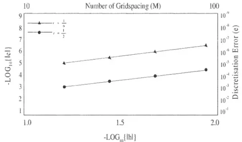
complete problem computed using (1.4) are used instead of those calculated using (2.7) the result shown in Figurel. indicate that this LOD procedure has produced only second order results, for s*=l/6 the slope of the line of best fit which gives an estimate of the order of convergence of the error, is 1.82 and for r*=l/2 it is 2.02.

The correct boundary values to be used along y=0 and y=N at the intermediate time level for the second half-time step are those obtained from the boundary values at the previous time tn by applying the one-dimensional finite-difference equation being used elsewhere in the interior of the region. Note that end-points values along x=Ü and x=M at the intermediate time level are not required in the second stage.

10 Number of Gridspacing (M) 100 9 ıır" _ı__ 8 1 10· 3 ~ f , c . -7 ıo 7 ""' ~ _---4 '-6 - - - 4 - - - ıo·h w ~

---

_--~---

_c:: ~ 5

..---

_l(i'; o

o

_____.,

__

__________.

_""

o

4 _ıo' ~ u; .-1

---

(l) ' ₃

---~---

10·l ı--a u vo 2 10' c:ı 1(/ 1.0 1.5 2.0 -LOGIO( lhl}

Figure 1. Relation between error u and gridspacing for exp.method with using (1.4)

A Studv On 9 Poiııı FTCS Two Level Dif[ereııce Methods With LOD Procedure M.GÜLSU

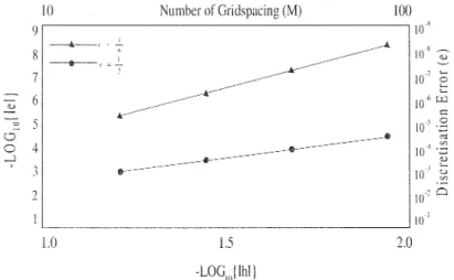
The numerical result obtained with this procedure are shown in Figure 2. It is clear that the errors when r*=l/6 are now of order fourth. In fact, the slope of the line of best fit for r*=l/6 is 4.01 while that for r*=l/2 is 2.02. This clearly shows that the correct treatment of the boundaries at the intermediate time level for any time-splitting procedure is very important in the generation of the final solution.

[() Number of Griclspacing (M) [()() 9 Hı" ---¾---' _---" ıo' ~ " - - - - @ - , 1

~---10 7 ,_ 7 _~

_g

6

---~

10 (, µı ...'!::

..

-

--

--- _:::: ~ ıo' -~ o --«> c j o 4

----~

_ıo'

_·.=

"7

___

________.--- :'::'. 3 &-··· _ıo·• u = 2 _ıo' 0 10·' 1.0 j j _2.0 -LOG,) llıl)

Figure 2. Relation between error u and gridspacing for exp. method with using (2.7) 3. THE (1,9) FTCS EQUATION

The 9-point fully explicit finite- difference rnethod uses a forward-difference approxirnation for the time derivative and following weighted approximation for the derivatives. Using the finite -difference approxirnation

a2ı:

;::;:

<p{ [

es

(i, j - 1, n)]

+ [

es

(i, j

+

1, n)]

+

(1- 2<p)[

es

(i, j,n )] (3.1)

ax

aa2~ ;::;: y{ [CS(i-1, j,n)]

+

[eS(i

+

1, j,n)]

+

(1-2y)[eS(i, j,n)] (3.2)

y-in which <p and

y

are weights which depend on rx and ry and CS is used to denote the second-order centred-difference approximation in the appropriate direction about the grid point.This differencing yields the explicit (1,9) FTCS difference equation:

ıı+l { } ( n n n 11)

ıti,j

=

{f)r,

+

rrv

Ui-1,j-l

+

Ui+l,j-1

+

Ui-1,j+I

+

Ui+!,j+I (3.3)

A Study Oıı 9 Poiııt FTCS Two Level Difference Metlıods Witlı LOD Procedııre M.GÜLSU

+ {

ry - 2( (f]rx

+

;»"y) }(ui,j-ı"

+

ui,j+I n)

+ {

r, -

2(

(flrx

+

;ı,r-Y) }(ui-1,/'

+

U;+ı./)

+

{l-2(rx

+

ry)

+

4((/Jrx

+

;»"y) }u;,/' These approximation can be written as follows:

au

aı n+I n

u..

_1,J

-u ..

_1,J

k

(3.4) :ı2 [ ( ıı 2 n ıı) ( ıı 2 n

n))

~x~

=

~

ui+l,j-1 - (~)~

+

ui-l,j-l

+

U;+ı,j+l

- (~;~

+

ui-1,j+I

+

(

u. ." - 2u . . " + u. .

il

J

+(1-rx) ı+l,J ( ~ ;₂ ,-ı., (3.5)

2 [ ( ıı 2 ıı n) ( n 2 ıı

n)]

Ö U

rv

U;-ı 1·+1 - U;-ı 1·

+

U;-ı 1·-1 U;+ı 1·+1 - U;+ı 1·

+

U;+ı 1·-ı

- = - ' - ' ' '

+

.

.

.

+

ayı ı

<~y)2

(~y)2

+(1-r )

₍

u. .

,,1+ı ,.1 ,.1-ı

11

-

2u. ."

+

u. .

il

J

y

(Ay)2

(3.6)

These approximations produce the following fınite-difference equation:

ıı+l ( ıı tı il " )

(1 2 )

U;,j

=

r_,ry

U;-ı,j-ı

+

U;-ı,j+ı

+

U;+ı,j-ı

+

U;+ı,j+ı

+

rY -

r.,

(u";,;-ı

+

u";,j+ı )

+

r_Jl-2ry)(u;-ı,/

+

U;+ı,/)

+

(l-2r_,)(1-2ry)u;,/ (_{3_7)}

If rx=ry=r, then (3.7) becomes

ıı+l 2( n ıı ıı ") (1 2 )

U;,j =

r

U;-ı,j-ı

+

U;-ı,j+ı

+

U;+ı,j-ı

+

U;+ı,j+ı

+

r -

r

(u .. _

l,] 111

+

u.

l,J •+ı")

+

r(l-

2r)(u._

1 1 •,] 11

+

u.

ı+ 1 .") ,J

+

(1-

2r)

2

u . . "

1,J (3.8)

The range of stability corresponding to (3.8) is O<

r ~

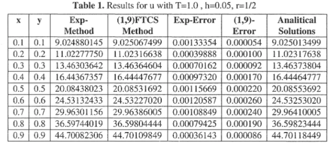
1/ 2

A Study On 9 Poiııt FTCS Two Level Differeııce Methods With LOD Procedure M.GÜLSU In Tablel the results are shown for ui,j n with L\x=L\y=h=0.05 and r=l/2 at

T=l.0 using explicit method and the (1,9) FfCS formula with given boundary values everywhere.

When the absolute value of the error;

e.

_n

=

u(ih, jk,nk)-u . . "

l,J l,J (3.9)

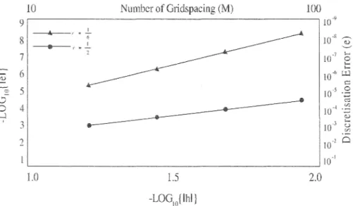
at the point (0.5,0.5) at time T=l.0 was graphed against h on a logarithmic scale for various of r it was found that the slope of lines was always close to 2 for 9-point FTCS formula. These results illustrate the theoretical orders of accuracy evident from the modified equivalent equation.

The numerical results obtained with the fourth-order one dimensional equation are shown in Figure 1. The slopes of the lines of best fit to the results are very close to 4 for each r. These results indicate that this fourth-order technique is much more accurate then the second-fourth-order method based on the FTCS formula. For example with r=l/2 and L\x=0.5 the error produced by tıie second -order method was about 10-4 _{while that produced}

by the fourth-order technique was about 10·1 .

10 Number of Gridspacing (M) 100 9 10-Y 1 8 /" = 6 10·8 ~ r r = - '--' 7 2 10•7 ı... o ... _... <1) 6 10·" ı:ı:ı ı::: o _{5 10·5}

.g

o

o:ı

o

4 10•4 -~ ....ı <1) ' ₃ 10·3 ... Ü -~ 2 10·2 Q J0-1 1.0 1.5 2.0 -LOG!O{lhl]

Figure 3. Relation between error u and gridspacing for 9-point FfCS method

A Study On 9 Poiııt FTCS Two Level Differeııce Metlıods With LOD Procedure M.GÜLSU

Table 1. Results for u with T=l.0, h=0.05, r=l/2

X y Exp- (1,9)FTCS Exp-Error (1,9)- Analitical

Method Method Error Solutions

0.1 0.1 9.024880145 9.025067499 0.00133354 0.000054 9.025013499 0.2 0.2 11.02277750 11.02316638 0.00039888 0.000100 11.02317638 0.3 0.3 13.46303642 13.46364604 0.00070162 0.000092 13.46373804 0.4 0.4 16.44367357 16.44447677 0.00097320 0.000170 16.44464777 0.5 0.5 20.08438023 20.08531692 0.00115669 0.000220 20.08553692 0.6 0.6 24.53132433 24.53227020 0.00120587 0.000260 24.53253020 0.7 0.7 29.96301156 29.96386005 0.00108849 0.000240 29.96410005 0.8 0.8 36.59744019 36.59804444 0.00079425 0.000190 36.59823444 0.9 0.9 44.70082306 44.70109849 0.00036143 0.000086 44.70118449

Overall, it can be seen that LOD techniques provide an effective solution to the two-dimensional problem. However, it must be kept in mind that proper treatment is required with the LOD procedure to obtain the correct values to be used on the boundary at intermediate time levels.

4.CONCLUSION

in this paper time-split finite difference method have been used to solve the two-dimensional constant coefficient diffusion equation with given boundary values. Using the Explicit method for one-dimensional diffusion equation in a LOD procedure with special treatment on the boundaries at the intermediate time level gave fourth-order accuracy. Without the special boundary treatment at the intermediate time levels high-order methods used at interior grid points in an LOD procedure only produce low-order results.

A comparison with the implicit scheme for the test problem clearly demonstrates that this technique are computationally superior. The numerical test obtained by using these methods give acceptable results. Also (1,9) FTCS method produced second-order results. it used more CPU time than the fourth-order LOD procedure to get results of the same accuracy.

A Stııdy On 9 Point FTCS Two Level Difference Methods With LOD Procedııre M.GÜLSU

REFERENCES

1. Ames W. F., Numerical Metlıods for Partial Differential Equations, Academic Press, New York, (1992).

2. Delıghan M., Implicit Locally One-Dimensional Metlıods for Two-Dimensional Diffusion witlı a Non-Local Boundary Condition, Matlı. And Computers in Simulation, 49(4), 331-349, (1999).

3. Herceg D., Cvetkovic L., On a Numerical Differentiation, SIAM J. Numer. Anal., 23 (3), 686-691, (1986).

4. Noye B. J., Hayman K. J., Explicit Two-Level Finite -Difference Metlıods for Tlıe Two-Dimensional Diffusion Equation, Intern.J.Computer Matlı., 42, 223-236, (1991).

5. Smitlı G. D., Numerical Solution of Partial Differantial Equations, Oxford Univ. Press, Oxford, (1985).

6. Vanaja V., Kellogg R. B., Iterative Metlıods for a Forward-Backward Heat Equation, SIAM J. Numer. Anal., 27 (3), 622-635, (1990).