DEVELOPING A SCORECARD
FOR CONSUMER CREDITS
MUSA BOĞAÇ DEVRİMCİ
106621015
İSTANBUL BİLGİ ÜNİVERSİTESİ
SOSYAL BİLİMLER ENSTİTÜSÜ
SAYISAL FİNANS YÜKSEK LİSANS PROGRAMI
ORHAN ERDEM
2009
BİREYSEL KREDİLERDE
KREDİ SKORLAMASI
M. Boğaç Devrimci
106621015
Tez Danışmanı :
Yrd. Doç. Dr. Orhan Erdem
Jüri Üyesi :
Doç. Dr. Ege Yazgan
Jüri Üyesi :
Yrd. Doç. Dr. Muzaffer Akat
Tezin Onaylandığı Tarih
: ...
Toplam Sayfa Sayısı: 30
Anahtar Kelimeler (Türkçe)
Anahtar Kelimeler (İngilizce)
1) Kredi Skorlama
1) Credit Scoring
2) Lojistik Regresyon
2) Logistic Regression
3) Bireysel Krediler
3) Consumer Credits
ABSTRACT
The purpose of this paper is to make a summary of the credit scoring techniques and to present two different credit application scoring models for vehicle and general purpose loans. We used logistic regression technique in developing our models and we used two different data sets for the two kinds of loans. After developing the models, we tried to define the cutoff score where applicants with scores greater than or equal to this score are accepted and others below this are rejected. In order to define the cutoff score, we constructed strategy curves for each credit type where the expected bad rate is plotted against the acceptance rate in order to show the tradeoffs between risk and volume.
Finally we have tested the results by using Receiver Operating Characteristic (ROC) curve and calculated the Gini coefficients.
Keywords: Credit Scoring, Logistic Regression, Consumer Credits
ÖZ
Bu çalışmanın amacı kredi skorlama teknikleri hakkında genel bir özet sunmak ve taşıt kredileri ile nakit ödemeli bireysel krediler için başvuru skorkart modelleri oluşturmaktır. Kredi skorlarının modellemesinde lojistik regresyon yöntemi kullanılmış olup, her bir kredi türü için ayrı veri kümeleri kullanılmıştır. Modellerin geliştirilmesinden sonra, üzerinde kalan kredi başvurularının olumlu; altında yer alan kredi başvurularının ise olumsuz olarak değerlendirildiği kesim puanları belirlenmiştir. Kesim puanlarının belirlenmesinde, risk ve hacim karşılaştırmasını yapabilmek için her bir kredi türü için beklenen temerrüt oranı ile beklenen kredi kabul oranlarının yer aldığı strateji doğruları oluşturulmuştur.
Sonuç olarak ise, model sonuçları ve model performansı ROC doğruları ile test edilip GINI katsayıları hesaplanmıştır.
i TABLE OF CONTENTS
I. INTRODUCTION ... 1
1. METHODOLOGIES FOR CLASSIFYING APPLICANTS ... 6
Logistic Regression ... 7
2. THE DATA ... 10
3. THE MODEL ... 13
A. Vehicle Loans ... 14
B. General Purpose Loans ... 16
4. THE MODEL PERFORMANCE ... 22
II. CONCLUSION ... 26
ii INDEX OF FIGURES
Figure 1.1 Graph of log (p/(1-p) ) ... 9
Figure 3.1 Strategy Curve of Vehicle Loans ... 20
Figure 3.2 Strategy Curve of General Purpose Loans ... 20
Figure 4.1 ROC Curve ... 23
Figure 4.2 ROC Curve of Vehicle Loans ... 24
Figure 4.3 ROC Curve of General Purpose Loans ... 25
INDEX OF TABLES Table 1.1 Comparison of classification accuracy for different scoring approaches ... 7
Table 2.1 Sample Size ... 10
Table 2.2 Characteristics Used In The Models ... 11
Table 2.3 Descriptive Statistics (Vehicle Loans) ... 12
Table 2.4 Correlation Matrix (Vehicle Loans) ... 12
Table 2.5 Descriptive Statistics (General Purpose Loans) ... 13
Table 2.6 Correlation Matrix (General Purpose Loans) ... 13
Table 3.1 Results Of Vehicle Loans ... 14
Table 3.2 Marginal Effect Analysis for Vehicle Loans (from biggest to smallest)... 16
Table 3.3 Results Of General Purpose Loans... 17
Table 3.4 Marginal Effect Analysis for General Purpose Loans (from biggest to smallest) ... 18
Table 3.5 Score Ranges ... 18
Table 3.6 Acceptance Rate & Bad Rate of Acceptance (Vehicle Loans) ... 21
Table 3.7 Acceptance Rate & Bad Rate of Acceptance (General Purpose Loans) ... 21
Table 3.8 Bad & Good Loans (Cutoff Point at Score 3) ... 21
Table 3.9 Bad & Good Loans (Cutoff Point at Score 3-Out Sample) ... 22
1
I.
INTRODUCTION
Many statistics can be used to show the enormous economic incentive for better techniques in credit management area. During the first quarter of 2008, bad debt amount of consumer credits in Turkey increased by 132% with respect to the same period of the previous year. 54 % of these credits consist of general purpose loans, 26 % consist of vehicle loans and 19 % consist of housing loans and 1% other type of credits1. After the financial crisis in Turkey, as of the end of September 2001, the rate of non-performing loans to total loans increased to 18,6 % from 9,3 % in September 2000. This situation and many other statistics force the financial services to develop better credit management tools.
Credit scoring is a decision support tool that aids credit lenders in the granting of credits and credit management. These tools are built to answer the question how likely is the applicant for credit to default by a given time in the future, by classifying the applicants as good and bad risks based on past statistical experience. The objective of analyzing the past is to find characteristics that significantly distinguish groups of applicants who are reliable debtors from those who are less reliable. In this technique a combination of criteria such as sex, age, marital status, profession, past credit history and several others yield a number called score which is assigned to an existing credit or to an applicant.
With the huge growth in consumer credits, credit scoring has become increasingly important. Especially, the arrival of credit cards in 1960s forced the financial services to realize the usefulness of credit scoring. The advantages of credit scoring can be summarized as;
lower transaction costs accelerating decision-making reducing bias
less manpower input lower delinquency ratios quantifiable risk management
2 Generally, credit scorecards can be considered to fall into two broad categories:
application scoring behavioral scoring
The techniques used to solve whether to grant credit to a new applicant are called application scoring. On the other hand, the techniques used to solve how to deal with the existing applicants are called behavioral scoring. The intent of application scoring is to forecast the future behavior of a new credit applicant, whereas behavioral scoring tries to predict the future payment behavior of an existing customer.
While the history of credit scoring goes back 50 years, the first approach to discriminating groups in a population was introduced in statistics by Fischer (1936). Fisher, aimed to find the combination of variables that best separated two groups whose characteristics were available. These two groups were different subspecies of a plant and the characteristics were the physical measurements. Durand (1941) was the first to recognize that one could use the same methods to discriminate between good and bad loans.
Beaver (1966, 1968) did univariate analysis of a number of bankruptcy predictors. He found that a number of indicators could discriminate between samples of default and non-default firms for as long as five years prior to failure.
Altman (1968) used a multivariate discriminant analysis with 5 variables for publicly traded manufacturing firms in the USA. Altman obtained 94% and 97% classification accuracy among default and non-default firms, respectively and 95% overall accuracy. Deakin (1972), applied discriminant analysis and the misclassification errors averaged 3 %, 4,5 % and 4,5 % for the first, second and third years before failure. He also tested the model on an independent sample consisting of 11 default and 23 non-default firms selected at random from Moody’s
3 Industrial Manual. Lane (1972) used 247 personal bankruptcy cases and 250 debt counselees2 with discriminant analysis. In his study, 93.2 % of personal bankruptcy cases were correctly classified, whereas for debt counselees this number was 94.78 %.
Different from credit scoring, Awh Waters (1974) used discriminant analysis in order to establish the extent to which differences exist between active and inactive bank charge cardholders in terms of selected economic, demographic, and attitudinal characteristics, and to ascertain the relative importance of various characteristics in differentiating between active and inactive cardholders. Moreover, Blum (1974) applied discriminant analysis in order to develop a credit scoring model. The predictive accuracy of his model was 93-95 % at the first year before default, 80 % at the second year, 70 % at the third, fourth and fifth years before default. One year later, Sinkey, then, Altman and Lorris (1976) acquire 90% classification accuracy with the help of five financial ratios. Another paper on discriminant analysis was published by Dambolena and Khory (1980).
After the development of the computer technology, methods applied in this area changed rapidly. During the 1970s the mostly used methods in credit scoring was regression based models. Firstly, the linear regression method was used and then because of the limitations of this method, logistic regression came into play.
Orgler (1970) used regression analysis for commercial loans and he classified 75 % of bad loans as bad and 35 % of good loans as good. In another study Orgler (1971) developed a behavioral scorecard. He concluded that in order to evaluate the credit portfolio quality behavioral characteristics are more predictive than the characteristics for application scorecards. Another regression based study was done by Fitzpatrick (1976). Other studies in which regression methods were used are Lucas (1992) and Henley (1995).
Wiginton (1980) studied logistic regression in a comparison with discriminant analysis. He conducted a study using data for credit applications of a major oil company. He concluded that
2 Debt counselees is the term used for persons who find they are having difficulty in repaying their debts and seek
4 maximum likelihood techniques for estimating the parameters of a logit probability function perform considerably better than the linear discriminant function. Srinivasan and Kim (1987) also compared logistic regression with other methods. Leonard (1993) used logistic regression for the evaluation of commercial loans. Olhson (1980), in his paper, investigated a logistic regression analysis. In his study 17.4 % of non-default firms and 12.4% of default firms were misclassified. Pantalone and Platt (1987) used logistic regression in their paper. They obtained 98% accuracy in the classification of failed firms and 92% accuracy in that of non-failed firms.
After 1990s statistical methods were replaced by the machine learning type methods like neural networks or recursive partitioning. Tam and Kiang (1992) applied discriminant analysis, logistic regression and neural networks with eighteen explanatory variables. Rosenberg and Gleit (1994) analyzed neural network technique in corporate credit decisions. Desai et al (1997) also compared the performance of neural network with logistic regression and discriminant analysis. Laitinen and Kankaanpaa (1999) compared discriminant analysis, logistic regression, recursive partitioning, survival analysis and neural networks. Mirta Bensic, Natasa Sarlijab and Marijana Zekic-Susac (2005) compared neural network with other methods.
As it is mentioned above, many studies in this area outline different modeling techniques that can be used to build such systems-discriminant analysis, linear regression, logistic regression, partitioning trees, mathematical programming, neural networks, expert systems and genetic algorithms. Whatever technique used, it is obvious that scoring model development involves statistical analysis of large amounts of data.
In this paper we used the term credit to refer to an amount of money loaned to a consumer by a financial institution which must be repaid with interest. Also, we used the term bad risk/bad credit for default customers and good risk/good credit for non-default customers.
The objective of this paper is to make a summary for the credit scoring techniques and to present two different credit application scoring models for vehicle and general purpose loans.
5 Although many classification techniques have been used in this area, the logistic regression has been used widely in studies. In this study, we also used logistic regression technique in order to discriminate between good and bad credits. The first chapter presents the widely used credit scoring techniques which are discriminant analysis, linear regression, logistic regression, classification trees and neural networks and briefly present some studies about the comparison of these methods. Also a brief mathematical theory behind logistic regression is analyzed. In the next two chapters we describe the data and the model we used in our study. After developing the models, finally in the fourth chapter we tested the performance of the scoring models with Receiver Operating Characteristic (ROC) curves.
6
1.
METHODOLOGIES FOR CLASSIFYING APPLICANTS
Historically, discriminant analysis and regression based models are the most widely used methods in credit scoring. Other techniques which are used in this area can be classified as;
Neural Networks Recursive Partitioning Nearest-neighbor approach Expert systems
Time varying models Linear Programming Integer Programming Genetic algorithms
Although different types of scoring techniques are listed above, studies showed that it is difficult to determine the best method. In fact, the decision of which method is the best depends on the details like data structure, characteristics used in the model, objective of the classification. For example, in situations where there is a poor understanding of data structure, neural networks techniques are very useful. Because, these systems combine automatic feature extraction with the classification process, which means that such methods can be used without a deep understanding of the problem. On the other hand, if we know the data and the problem very well, methods which use this knowledge might be expected to perform better results. The fact that many studies are made in credit scoring on similar data can be interpreted as a good understanding of this technique. This might explain why neural networks have not been used regularly in this sector (Hand and Henley, 1997).
7
Table 1.1 Comparison of classification accuracy for different scoring approaches
Authors Linear reg. Logistic reg. Class. trees LP NN GA
Srinivisian (1987) 87.5 89.3 93.2 86.1 - -
Boyle (1992) 77.5 - 75.0 74.7 - -
Henley (1995) 43.4 43.3 43.8 - - -
Yobas (1997) 68.4 - 62.3 - 62.0 64.5
Desai (1997) 66.5 67.3 - - 66.4 -
Thomas, Lyn C., Edelman, David B., Crook, Jonathan N. (2002) Credit scoring and its applications. Philadelphia: SIAM (Society for Industrial and Applied Mathematics)
The values in the table are the percentage of the correctly classified data. According to Srinivisian (1987) and Henley (1995) classification trees are the best methods. On the other hand, in Boyle (1992) and Yobas (1997) work, linear regression is the best, whereas Desai (1997) concluded that logistic regression is the best.
Mirta Bensic, Natasa Sarlijab and Marijana Zekic-Susac (2005) compared the accuracy of the best models for small business extracted by different methodologies, such as logistic regression, neural networks (NNs), and CART decision trees. Their results showed that the highest total hit rate and the lowest type I error are obtained in Neural Network. In a comparative study, Henley (1995) found that logistic regression isn’t better than linear regression.
Logistic Regression
Logistic regression is a kind of regression which is used when the dependent variable is a binary or dichotomous and the independents are of any type. In logistic regression, one matches the log of probability odds by a linear combination of the characteristics variables; i.e.,
Log ( ) = w0 + w1x1 + w1x1 + …+ wpxp = w xT
8
pi =
which is the logistic regression assumption. If we assume that the means are µG (goods) and µB
(bads) with common covariance matrix ∑. Then, E (Xi| G) = µG,i
E (Xi| B) = µB,i
E (Xi Xj| G) = E (Xi Xj| B) = ∑ij
In this case the density function is; f(x|G) = (2π)-p/2
(det∑)-1/2 exp
where (x-µG) is a vector with 1 row and p columns and (x-µG)T is its transpose. If we assume
that PB is the proportion of the population of bads and PG is the proportion of the population of
goods, then the log of the probability odds for customer i who has characteristics x is;
log ( ) = log ( )
= x 2(µB - µG)T+ (µG + µB ) + log (PG / PB)
As this is the linear combination of xi, it satisfies the logistic regression assumption. Below is
the case where the characteristics are all binary and independent of each other. P(Xi = 1|G) = PG(i) P(Xi = 0|G) = 1 – PG(i);
P(Xi = 1|B) = PB(i) P(Xi = 0|B) = 1 – PB(i);
If PG, PB are the prior of goods and bads;
P(G|x) = =
Log ( ) = ∑i xi log(PG (i)) – log(PB (i) )) + ∑i (1-xi) (log(1-PG(i)) - log(1-PB(i))) + log(
9 This also satisfies the logistic regression assumption.
The ordinary least squares approach cannot be used in logistic regression in order to calculate the coefficients w. Maximum likelihood approach has to be used to get the coefficients.
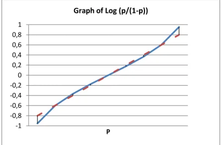
Figure 1.1 Graph of log (p/(1-p) )
Some advantages of logistic regression can be listed as; Scores are interpretable in terms of log odds.
It does not need a linear relationship between the independent and dependent variable. The Dependent Variable need not be normally distributed.
It is more robust.
On the other hand, the requirement of the high data size in order to obtain meaningful results can be regarded as a disadvantage of this method.
According to Sarantopoulos (2003); the logistic regression model overcomes the criticism of the linear regression model in three ways. First, the response (or outcome) is assumed to be binomially distributed. Second, the model restricts the output to lie between 0 and 1. Third, the curve of logit is a special s-shaped (sigmoid) curve and symmetric about p=0.5.
-1 -0,8 -0,6 -0,4 -0,2 0 0,2 0,4 0,6 0,8 1 P Graph of Log (p/(1-p))
10
2.
THE DATA
The data used in this study was collected randomly from a financial services firm. The major problem in obtaining data was the lack of some characteristics of the applicants. Although there are many statistical methods to cope with missing characteristics in discrimination, we eliminated the data with missing characteristics and did not use such methods. All of the credits used in the data are granted between year 2002 and 2007, which are closed as of 2009. We did not use credit data granted before 2002 in order to reduce the effect of the financial crisis occurred in 2001 in Turkey. In order to obtain sufficient number of data, thousands of applicants were screened and analyzed. We tried to develop a model relating to the population of applications including the accepted and rejected customers. However, we can only observe the repayment performance for those who were accepted. As we cannot observe the repayment performance for the rejected applicants we could not use those applicants in our study.
Because of the different characteristics among vehicle3 and general purpose4 loans we tried to develop separate models. In fact that we aimed to develop separate models for vehicle and general purpose loans, we used different samples for each of the credit types.
The sample sizes used in our study are given below.
Table 2.1 Sample Size
Credit Type Sample Size # of Good Credits # of Bad Credits
Vehicle Loans 8.320 6.146 2.174
General Purpose Loans 8.327 6.410 1.917
Firstly, 35 different characteristics were tried to be used, but because of the insufficient data quality 19 characteristic were neglected and 16 characteristics were included. Most of the characteristics describe the credit applicants profile and income status. An applicant was
3 Vehicle Loans: This type of loan is used to finance the purchase of a new or previously owned car. The maximum loan maturity is 36 months.
4
General Purpose Loans: This type of loan is used to finance all personal needs from a holiday to home appliances, emergency health expenses to in vitro fertilization. The maximum loan maturity is 36 months.
11 classified as good and bad according to the payment performance. The characteristics used in the model are given below.
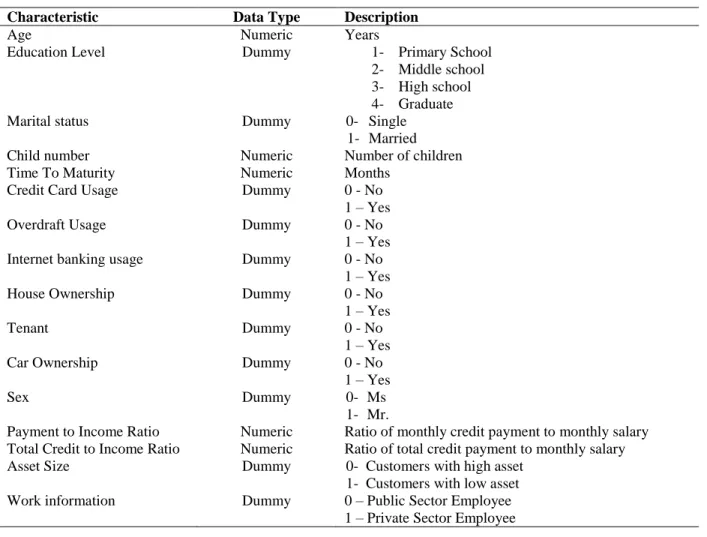
Table 2.2 Characteristics Used In The Models
Characteristic Data Type Description
Age Numeric Years
Education Level Dummy 1- Primary School
2- Middle school 3- High school 4- Graduate
Marital status Dummy 0- Single
1- Married
Child number Numeric Number of children
Time To Maturity Numeric Months
Credit Card Usage Dummy 0 - No
1 – Yes
Overdraft Usage Dummy 0 - No
1 – Yes
Internet banking usage Dummy 0 - No
1 – Yes
House Ownership Dummy 0 - No
1 – Yes
Tenant Dummy 0 - No
1 – Yes
Car Ownership Dummy 0 - No
1 – Yes
Sex Dummy 0- Ms
1- Mr.
Payment to Income Ratio Numeric Ratio of monthly credit payment to monthly salary
Total Credit to Income Ratio Numeric Ratio of total credit payment to monthly salary
Asset Size Dummy 0- Customers with high asset
1- Customers with low asset
Work information Dummy 0 – Public Sector Employee
1 – Private Sector Employee
All of the variables except age, child number, time to maturity and salary are dummy variables. The descriptive statistics for vehicle loans are given below.
12
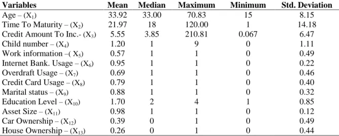
Table 2.3 Descriptive Statistics (Vehicle Loans)
Variables Mean Median Maximum Minimum Std. Deviation
Age – (X1) 33.92 33.00 70.83 15 8.15
Time To Maturity – (X2) 21.97 18 120.00 1 14.18
Credit Amount To Inc.- (X3) 5.55 3.85 210.81 0.067 6.47
Child number – (X4) 1.20 1 9 0 1.11
Work information –( X5) 0.57 1 1 0 0.49
Internet Bank. Usage – (X6) 0.95 1 1 0 0.22
Overdraft Usage – (X7) 0.69 1 1 0 0.46
Credit Card Usage – (X8) 0.79 1 1 0 0.40
Marital status – (X9) 0.88 1 1 0 0.32
Education Level – (X10) 1.70 2 4 1 0.85
Asset Size – (X11) 0.98 1 1 0 0.12
Car Ownership – (X12) 0.39 0 1 0 0.49
House Ownership – (X13) 0.26 0 1 0 0.44
It can be seen from the above table that the average age of the customer data used is 33.92, where the oldest one is 70.83 and the youngest is 15 years old. The correlation matrix of 13 variables is given below.
Table 2.4 Correlation Matrix (Vehicle Loans)
X1 X2 X3 X4 X5 X6 X7 X8 X9 X10 X11 X12 X13 X1 1.00 -0.02 0.03 0.31 0.00 -0.07 -0.01 0.03 0.19 -0.01 -0.10 0.17 0.25 X2 -0.02 1.00 0.45 0.00 -0.10 -0.08 -0.19 -0.10 0.02 0.09 0.06 -0.08 -0.07 X3 0.03 0.45 1.00 -0.00 -0.01 -0.06 -0.14 -0.08 -0.01 0.07 0.01 -0.03 -0.02 X4 0.31 0.00 -0.00 1.00 0.00 0.02 0.06 0.08 0.37 0.11 -0.02 0.13 0.09 X5 0.00 -0.10 -0.01 0.00 1.00 0.08 0.02 0.06 -0.02 0.07 -0.05 0.10 0.07 X6 -0.07 -0.08 -0.06 0.02 0.08 1.00 0.22 0.18 -0.01 -0.15 -0.02 0.13 0.06 X7 -0.01 -0.19 -0.14 0.06 0.02 0.22 1.00 0.40 0.05 -0.20 -0.06 0.16 0.09 X8 0.03 -0.10 -0.08 0.08 0.06 0.18 0.40 1.00 0.04 -0.14 -0.05 0.12 0.08 X9 0.19 0.02 -0.01 0.37 -0.02 -0.01 0.05 0.04 1.00 0.09 -0.00 0.11 0.03 X10 -0.01 0.09 0.07 0.11 0.07 -0.15 -0.20 -0.14 0.09 1.00 0.07 -0.23 -0.16 X11 -0.10 0.06 0.01 -0.02 -0.05 -0.02 -0.06 -0.05 -0.00 0.07 1.00 -0.11 -0.10 X12 0.17 -0.08 -0.03 0.13 0.10 0.13 0.16 0.12 0.11 -0.23 -0.11 1.00 0.31 X13 0.25 -0.07 -0.02 0.09 0.07 0.06 0.09 0.08 0.03 -0.16 -0.10 0.31 1.00
13 The descriptive statistics for general purpose loans are given below.
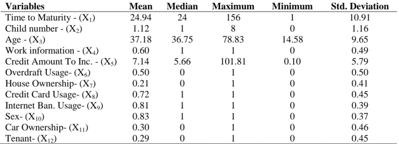
Table 2.5 Descriptive Statistics (General Purpose Loans)
Variables Mean Median Maximum Minimum Std. Deviation
Time to Maturity - (X1) 24.94 24 156 1 10.91
Child number - (X2) 1.12 1 8 0 1.16
Age - (X3) 37.18 36.75 78.83 14.58 9.65
Work information - (X4) 0.60 1 1 0 0.49
Credit Amount To Inc. - (X5) 7.14 5.66 101.81 0.10 5.79
Overdraft Usage- (X6) 0.50 0 1 0 0.50
House Ownership- (X7) 0.21 0 1 0 0.41
Credit Card Usage- (X8) 0.72 1 1 0 0.45
Internet Ban. Usage- (X9) 0.81 1 1 0 0.39
Sex- (X10) 0.83 1 1 0 0.37
Car Ownership- (X11) 0.30 0 1 0 0.46
Tenant- (X12) 0.29 0 1 0 0.45
It can be seen from the above table that the average time to maturity of the credit data used is 24.94, where the minimum term is 1 and the maximum term is 156 months. The correlation matrix of 12 variables is given below.
Table 2.6 Correlation Matrix (General Purpose Loans)
X1 X2 X3 X4 X5 X6 X7 X8 X9 X10 X11 X12 X1 1.00 0.02 -0.06 -0.17 0.32 -0.01 -0.08 -0.05 -0.05 -0.00 -0.10 0.07 X2 0.02 1.00 0.23 -0.02 0.02 0.05 0.09 0.04 0.01 0.14 0.13 -0.00 X3 -0.06 0.23 1.00 0.13 0.05 0.01 0.19 0.07 -0.07 0.05 0.12 -0.15 X4 -0.17 -0.02 0.13 1.00 -0.02 0.00 0.13 0.05 0.08 -0.05 0.14 -0.10 X5 0.32 0.03 0.06 -0.02 1.00 0.02 0.01 0.001 -0.01 -0.05 -0.01 -0.00 X6 -0.02 0.05 0.01 0.002 0.02 1.00 0.07 0.33 0.16 -0.00 0.12 0.00 X7 -0.08 0.09 0.19 0.13 0.01 0.06 1.00 0.07 0.09 -0.02 0.31 -0.09 X8 -0.05 0.04 0.07 0.04 0.00 0.33 0.07 1.00 0.10 0.01 0.13 -0.04 X9 -0.05 0.01 -0.07 0.08 -0.01 0.16 0.09 0.10 1.00 -0.06 0.13 0.01 X10 -0.00 0.14 0.05 -0.05 -0.05 -0.00 -0.02 0.01 -0.06 1.00 -0.003 -0.01 X11 -0.10 0.13 0.12 0.14 -0.01 0.12 0.31 0.13 0.13 -0.00 1.00 -0.08 X12 0.07 -0.00 -0.15 -0.10 -0.00 0.00 -0.09 -0.04 0.01 -0.01 -0.08 1.00
3.
THE MODEL
As we mentioned before, logistic regression analysis is used to develop the model where the dependent variable is restricted to the values of zero for good credits and one for bad credits. Regression analysis was performed on a sample of good and bad loans where independent variables represent various characteristics of each applicant.
14
Y = 1 bad credits (default credits)
Y = 0 good credits (non-default credits)
In this study we tried to develop two different logistic regression models for vehicle and general purpose loans. After omitting all the variables that do not add to the explanation of variation in the dependent variable (Yi) and that are not significantly related to the dependent
variable, the equation of the best discrimination between good and bad credits is obtained. The results are given below.
A. Vehicle Loans
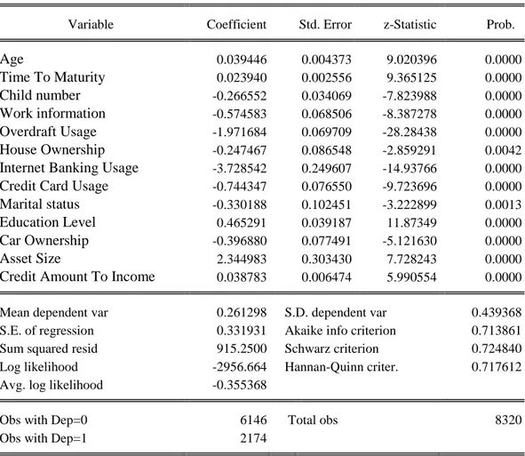
The equation results which show the coefficients and probabilities are shown below.
Table 3.1 Results Of Vehicle Loans Dependent Variable: B_G
Method: ML - Binary Logit (Quadratic hill climbing)
Variable Coefficient Std. Error z-Statistic Prob.
Age 0.039446 0.004373 9.020396 0.0000 Time To Maturity 0.023940 0.002556 9.365125 0.0000 Child number -0.266552 0.034069 -7.823988 0.0000 Work information -0.574583 0.068506 -8.387278 0.0000 Overdraft Usage -1.971684 0.069709 -28.28438 0.0000 House Ownership -0.247467 0.086548 -2.859291 0.0042
Internet Banking Usage -3.728542 0.249607 -14.93766 0.0000
Credit Card Usage -0.744347 0.076550 -9.723696 0.0000
Marital status -0.330188 0.102451 -3.222899 0.0013
Education Level 0.465291 0.039187 11.87349 0.0000
Car Ownership -0.396880 0.077491 -5.121630 0.0000
Asset Size 2.344983 0.303430 7.728243 0.0000
Credit Amount To Income 0.038783 0.006474 5.990554 0.0000
Mean dependent var 0.261298 S.D. dependent var 0.439368
S.E. of regression 0.331931 Akaike info criterion 0.713861
Sum squared resid 915.2500 Schwarz criterion 0.724840
Log likelihood -2956.664 Hannan-Quinn criter. 0.717612
Avg. log likelihood -0.355368
Obs with Dep=0 6146 Total obs 8320
15 Age is a variable which is not restricted to “0” or “1”. The positive coefficient implies that older applicants are more likely to default.
Time to maturity has a positive coefficient which means that as the maturity increases the probability of an applicant to default increases. This conclusion proves the fact that as the maturity increases the credit becomes more risky.
Child number is another variable which is not restricted to “0” and “1”. The negative coefficient implies that as the number of children increases the default probability of an applicant decreases. This is also consistent with our expectations, because number of children is directly related with the income level.
Work information variable is equal to “1” for private sector employees and “0” for public sector employees. So the negative coefficient of this variable implies that private sector employees are less likely to default.
Overdraft and credit card usage variables have negative coefficients. Both variables are equal to “1” for applicants who use these instruments and “0” for who do not. These results state that increased usage of banking instruments has an opposite effect on the probability of default.
House Ownership variable is equal to “1” for applicants who are the owner of a house and “0” for applicants who are not. Since the dependent variable is “0” for good loans and “1” for bad loans, the negative coefficient means that applicants who are house owners are less likely to default. This conclusion is obvious because house ownership is a sign of the income level of an applicant.
Internet banking usage is equal to “1” for applicants who use internet and “0” for who do not. The negative coefficient for this characteristic is also an expected result, because internet banking usage is related with income and education level of an applicant.
The coefficient of marital status is negative which means that married customers are less likely to default.
Education level variable has four categories mentioned in the previous section. The positive coefficient of the education level implies that while the education level increases the default probability of an applicant decreases.
16 Car ownership has a negative coefficient. This variable is equal to “1” for applicants who owns a car and “0” for who does not. This result is meaningful, because car ownership is a sign of high income level which has an opposite effect on the probability of default.
Asset size variable is equal to “1” for customers with low asset and “0” for customers with high asset. The positive coefficient means that as the asset size increases the default probability decreases.
Credit amount to income ratio variable has a positive coefficient. This means that when the ratio increases the likelihood of default also rises.
We have also made marginal effect analysis for the variables. The effect sizes of the variables are given below.
Table 3.2 Marginal Effect Analysis for Vehicle Loans (from biggest to smallest) Ranking Variable
1 Internet Banking Usage 2 Asset Size
3 Overdraft Usage
4 Age
5 Education Level 6 Credit Card Usage 7 Time To Maturity 8 Child number 9 Work information 10 Marital status
11 Credit Amount To Income 12 Car Ownership
13 House Ownership
It can be seen from the table that the biggest marginal effect belongs to internet banking usage, asset size and overdraft usage. On the other hand the lowest effect can be seen for house ownership and car ownership variables.
B. General Purpose Loans
After omitting the insignificant variables and regenerating the model we got the following results with 12 variables.
17
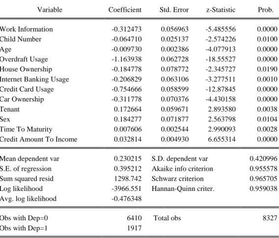
Table 3.3 Results Of General Purpose Loans
Dependent Variable: B_G
Method: ML - Binary Logit (Quadratic hill climbing) Sample: 1 8327
Included observations: 8327
Convergence achieved after 5 iterations
Covariance matrix computed using second derivatives
Variable Coefficient Std. Error z-Statistic Prob.
Work Information -0.312473 0.056963 -5.485556 0.0000
Child Number -0.064710 0.025137 -2.574226 0.0100
Age -0.009730 0.002386 -4.077913 0.0000
Overdraft Usage -1.163938 0.062728 -18.55527 0.0000
House Ownership -0.184778 0.078772 -2.345727 0.0190
Internet Banking Usage -0.206829 0.063106 -3.277511 0.0010
Credit Card Usage -0.754666 0.058599 -12.87845 0.0000
Car Ownership -0.311778 0.070376 -4.430158 0.0000
Tenant 0.172664 0.059671 2.893580 0.0038
Sex 0.184277 0.071877 2.563798 0.0104
Time To Maturity 0.007606 0.002544 2.990093 0.0028
Credit Amount To Income 0.032814 0.004930 6.655314 0.0000
Mean dependent var 0.230215 S.D. dependent var 0.420996
S.E. of regression 0.395212 Akaike info criterion 0.955578
Sum squared resid 1298.742 Schwarz criterion 0.965705
Log likelihood -3966.551 Hannan-Quinn criter. 0.959038
Avg. log likelihood -0.476348
Obs with Dep=0 6410 Total obs 8327
Obs with Dep=1 1917
The results for the general purpose loans are nearly consistent with the results of the vehicle loans. When we compare the variables, it can be seen that marital status, education level and asset size became insignificant for general purpose loans. On the other hand the variables of tenant and sex became significant for general purpose loans.
18
Table 3.4 Marginal Effect Analysis for General Purpose Loans (from biggest to smallest) Ranking Variable
1 Overdraft Usage 2 Credit Card Usage
3 Age
4 Credit Amount To Income 5 Time to Maturity
6 Work information 7 Internet Banking Usage
8 Sex
9 Car Ownership 10 Child number 11 Tenant
12 House Ownership
Defining the Score Ranges and the Cutoff Point
After developing the models, we tried to define score ranges and set a cutoff point for each of the credit types. Risk scores are used to evaluate the relative odds of binary Good/Bad outcomes of the random performance of an applicant. In our study, we used a methodology where risk increases as score increases. The scores we defined according to the probability of default values are given below.
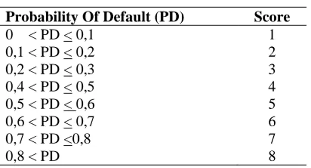
Table 3.5 Score Ranges
Probability Of Default (PD) Score
0 < PD < 0,1 1 0,1 < PD < 0,2 2 0,2 < PD < 0,3 3 0,4 < PD < 0,5 4 0,5 < PD < 0,6 5 0,6 < PD < 0,7 6 0,7 < PD <0,8 7 0,8 < PD 8
Cutoff point is a score where applicants with risk scores smaller than this point are accepted and others below this point are rejected. Many factors can be taken into consideration in order to set a cutoff point. These are profit, market strategy, acceptance rate, bad rate, expected loss etc. As profit is often the most important factor behind a scorecard cutoff decision, operational factors should also be considered. For example, if we decrease the cutoff point, an increase in
19 the acceptance rate occurs. As a result of this, the credit agency should have sufficient operational capacity (technology, infrastructure, labor force etc) in order to deal with more cases being fulfilled, more applications, more customer queries etc.
According to R.M. Oliver and E. Wells (2001), cutoff decision policies can be based on either single stage decision rules or on a more complex two-stage decision rule. In the two stage decision rule policy, the first stage is to;
Accept (above an upper cutoff point) Reject (below a lower cutoff point)
Leave Undecided (between the lower and upper cutoff points)
the application. In the second stage accept or reject decision is based on further information gathered for the applicant. In practice, sharp cutoffs are not always implemented, as there may be additional information available about the applicants. In this paper we focus on a single-stage decision policy.
Although there are many different ways in which a scorecard can be used to influence decisions that reduce risk and increase profitability of a credit portfolio, many policies do not require the direct use of economic data.
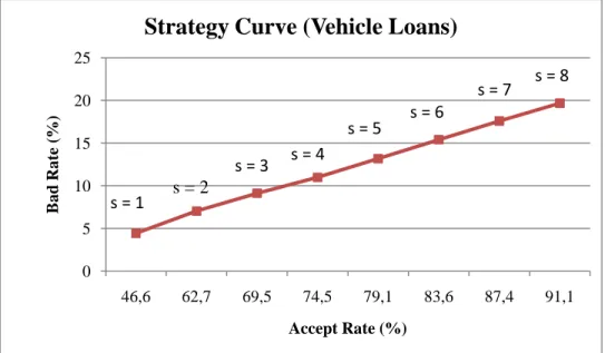
Strategy curve, which shows the expected bad rate plotted against the acceptance rate for various cutoff scores, is very useful in the decision of the cutoff point. This curve estimates various bad rates if a cutoff score is used in an acceptance rate measured on the x axis. The bottom left-hand part of the curve corresponds to large cutoffs and small acceptance rates, whereas the upper right-hand part of the curve corresponds to low cutoff points with high acceptance rates. Different scoring methods produce different strategy curves. This curve is very useful in order to analyze the tradeoffs between risk and volume.
As a practical matter, one does not need elaborate utility or preference models to analyze the effect of cutoff policies on statistical measures of Good/Bad outcomes and acceptance rates. Different cutoff points are tried, the resulting bad and acceptance rates are compared and, by trial and error, a solution that trades off a credit portfolio manager's loss exposure with management demands for larger portfolio sizes is obtained.
20 The strategy curves for the models we developed in this paper are given below.
Figure 3.1 Strategy Curve of Vehicle Loans
Figure 3.2 Strategy Curve of General Purpose Loans
It can be seen from figure 3.1 that, when s=1 is defined as the cutoff point, the accept rate is expected to be 46,6 % and the bad rate is expected to be 4,4 %. This means that when s=1 is defined as the cutoff point, 47 of 100 applicants will be granted credit and two of these
0 5 10 15 20 25 46,6 62,7 69,5 74,5 79,1 83,6 87,4 91,1 B a d Ra te (%) Accept Rate (%)
Strategy Curve (Vehicle Loans)
0 5 10 15 20 25 24,1 51,4 69,8 83,6 93,0 98,8 99,9 100,0 B a d Ra te (%) Accept Rate (%)
Strategy Curve (General Purpose Loans)
s = 1 s = 2 s = 3 s = 4 s = 5 s = 6 s = 7 s = 8 s = 1 s = 2 s = 3 s = 4 s = 5 s = 6 s = 7 s = 8
21 accepted applicants are expected to default. When we look at the strategy curve of general purpose loans, the accept rate is expected to be 24,1 % and the bad rate is expected to be 5,7 %. In other words, 24 out of 100 applicants will be granted credit and one of these accepted applicants are expected to default. The bad rates for each of the credit types are very close, whereas the acceptance rate for general purpose loans increases higher at lower cutoff points.
Table 3.6 Acceptance Rate & Bad Rate of Acceptance (Vehicle Loans)
Score Rejected # of Credits Accepted # of Credits Accepted # of Good Credits Accepted # of Bad Credits Acceptance Rate (%) Bad Rate Percent of Acceptance (%) 1 4.446 3.874 3.702 172 46,6 4,4 2 3.104 5.216 4.849 367 62,7 7,0 3 2.534 5.786 5.258 528 69,5 9,1 4 2.123 6.197 5.516 681 74,5 11,0 5 1.739 6.581 5.714 867 79,1 13,2 6 1.361 6.959 5.887 1072 83,6 15,4 7 1.050 7.270 5.992 1278 87,4 17,6 8 737 7.583 6.091 1492 91,1 19,7
Table 3.7 Acceptance Rate & Bad Rate of Acceptance (General Purpose Loans)
Score Rejected # of Credits Accepted # of Credits Accepted # of Good Credits Accepted # of Bad Credits Acceptance Rate (%) Bad Rate Percent of Acceptance (%) 1 6.324 2.003 1.889 114 24,1 5,7 2 4.045 4.282 3.821 461 51,4 10,8 3 2.516 5.811 4.952 859 69,8 14,8 4 1.368 6.959 5.681 1278 83,6 18,4 5 586 7.741 6.112 1629 93,0 21,0 6 104 8.223 6.363 1860 98,8 22,6 7 12 8.315 6.406 1909 99,9 23,0 8 1 8.326 6.409 1917 100,0 23,0
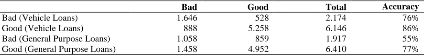
Table 3.8 Bad & Good Loans (Cutoff Point at Score 3)
Bad Good Total Accuracy
Bad (Vehicle Loans) 1.646 528 2.174 76%
Good (Vehicle Loans) 888 5.258 6.146 86%
Bad (General Purpose Loans) 1.058 859 1.917 55%
22 When we set the cutoff point at C=0.3 (s=3) we can see that 528 of the actually bad loans were classified as good and 1.646 as bad for vehicle loans. For general purpose loans 859 of the actually bad loans were classified as good and 1.058 as bad. Also 888 of the actually good vehicle loans were classified as bad and 1.458 of the actually good general purpose loans were classified as bad.
The test of the original sample is biased because the regression equation is based on the same data. A more powerful test can be obtained by using the model to classify the observations in the hold-out sample whose results are given below.
Table 3.9 Bad & Good Loans (Cutoff Point at Score 3-Out Sample)
Bad Good Total Accuracy
Bad (Vehicle Loans) 89 45 134 65%
Good (Vehicle Loans) 93 264 357 74%
Bad (General Purpose Loans) 64 62 126 51%
Good (General Purpose Loans) 112 262 374 70%
When we look at the results it can be seen that the accuracy ratio is lower than the results of the test made with the original data.
4. THE MODEL PERFORMANCE
Scorecard performance is the ability of the scoring methodology to rank or predict risk of a binary outcome. There are many ways to measure the scorecard performance. These measure how well the scorecard separates the two groups of good and bad credits. Measures of mean squared error, Brier score, divergence, Kolmogorov-Smirnoff (K-S) statistic, Gini Coefficient, Receiver Operating Characteristic (ROC) curve are some of the different techniques. In this study we used Gini coefficient to evaluate the performance and displayed the results in terms of a ROC curve.
The methods mentioned above measure the statistical performance of the scoring model and do not incorporate business objectives (profit, volume etc). Nevertheless, ROC curve has dominance properties equivalent to the dominance of efficient frontiers derived from business
23 objectives, such as expected loss, profit and portfolio size (Beling, P., Covaliu, Z., Oliver, R.M., 2005).
ROC curve is a plot of the cumulative proportion of true good risk against cumulative proportion of true bad risk as the threshold varies. An ideal classifier in such a plot would follow the axes, and the area between the curve and axes is sometimes used as a measure of discriminatory power of the scorecard. In other words, the best scorecard would have a curve that goes all the way along the horizontal axis before going up the vertical axis. K-S statistic is the maximum vertical distance between the ROC curve of a discriminating score and the ROC curve of a non-discriminating predictor.
ROC curve is also a useful tool in order to identify optimal cutoff scores. According to P Beling, Z. Covaliu, R.M. Oliver (2005), maximum expected profit is obtained with one of three policies: accept all applicants, reject all applicants, or determine a cutoff point and admit applicants only if their score exceeds this point.
If nG(s) and nB(s) are the numbers of goods and bads with score s in a sample of n, where there
are nG goods and nB bads
PG(s) = PB(s) =
Figure 4.1 ROC Curve
0 % Goods Rejected % Bads Rejected High Cutoffs Low Cutoffs C B A (100%) No Discrimination Perfect Discrimination 100%
24 are the probabilities of a good (and bad) having a score s.
An ROC curve along the diagonal 0B would correspond to one where at every score PG (s) =
PB (s), so the ratio of goods to bads is the same for all score ranges. The origin (0,0)
corresponds to the point where every applicant being accepted, that is, the lowest possible cutoff, and the point B (1,1) corresponds to the highest possible cutoff, where every applicant is rejected. For low cutoffs, the number of Bads rejected is small; as the score cutoff increases, a disproportionately large fraction of Bads (relative to the fraction of Goods) is rejected. A ROC curve with a shape of diagonal line connecting point 0 to the point B which corresponds to a classifier that has no discriminating power, that is, where one selects applicants at random. The ROC curves of the three models we have developed are given below.
25
Figure 4.3 ROC Curve of General Purpose Loans
The Gini statistic is a linear combination of the area under the trade off curve. It can be derived as follows:
Gini statistic = 2 * (ROC area - 0.5)
A high Gini value would mean that the model is separating goods from bads better than the random model. In figure 4.1 the perfect classifier that goes through point A will have Gini coefficient equal to 1. While the random classifier that goes through OB has Gini coefficient equal to 0.
Table 4.1 Gini Coefficients
Credit Type ROC Area Gini Coefficient
Vehicle Loans 0.8869 0.7733
General Purpose Loans 0.7379 0,4758
The Gini coefficients show that the discrimination power of the model we have developed for the vehicle loans is better than the one for general purpose loans.
26
II.
CONCLUSION
The increase in the Non-Performing Loan (NPL) ratio of financial services in Turkey forces the credit services to develop better credit management tools. Moreover, the huge growth in the credit portfolios enhances the necessity of using statistical or non-statistical methods in credit granting and credit monitoring processes. Credit scoring models are used for decades by financial services in order to accelerate the decision making process, reduce costs and manage risks more effectively. They were built to answer the question how likely is the applicant for credit to default by a given time in the future, by classifying the applicants as good and bad risks based on past statistical experience. In spite of the various number of methods used in credit scoring, all such methods try to predict a single outcome variable c (score) from a set of predictor variables.
In general credit scorecards can be considered to fall into two broad categories which are application scoring and behavioral scoring. The techniques used to solve whether to grant credit to a new applicant are called application scoring. Whereas, the techniques used to how to deal with the existing applicants are called behavioral scoring.
We used two different data sets and logistic regression method in developing the models. The data used in this study was collected randomly from a financial services firm. All the data consists of credits granted between year 2002 and 2007. We did not use credit data granted before 2002 in order to reduce the effect of the financial crisis occurred in 2001 in Turkey. In order to obtain sufficient number of data, thousands of applicants were screened and analyzed. When we compare the results of the models we found that the regression model for general purpose loans which provided the best discrimination between good and bad credits included only 12 variables. On the other hand, the number of significant variables for vehicle loans was 13.
After developing the models, we plot the strategy curves for both model in order to analyze the acceptance rates with respect to bad rates at different scores. Finally we plotted the ROC curves and calculated Gini coefficients to measure the performance of the scorecards. The
27 results and performance measures of the scorecards show that the discrimination power of the model we have developed for the vehicle loans is better than the general purpose loans.
28
REFERENCES
Altman, E. I. (1968), Financial Ratios, Discriminant analysis and the prediction of corporate bankruptcy, The Journal of Finance, 589-609.
Altman, E.I. and Loris, B. (1976), A financial early warning system for over the counter broker dealers, Journal of Finance, 31, 4, 1201-1217.
Awh, R. Y. and Waters, D. (1974), A discriminant analysis of economic, demographic, and attitudinal characteristics of bank charge card holders: a case study. Journal of Finance, 29, 973-980.
Beling, P., Covaliu, Z., Oliver, R. M. (2005), Optimal Scoring Cutoff Policies and Efficient Frontiers, The Journal of the Operational Research Society, Vol. 56, No. 9, 1016-1029. Blum, M., (1974) Failing company discriminant analysis, Journal of Accounting Research,
1-25.
Boyle, M., Crook, J. N., Hamilton, R. and Thomas, L. C. (1992), Methods for credit scoring applied to slow payers, Credit Scoring and Credit Control, Oxford University Press, 75-90.
Coffman, J. Y. (1986), The proper role of tree analysis in forecasting the risk behavior of borrowers, MDS Reports, Management Decision Systems, Atlanta, 3, 4, 7, and 9. Dambolena, I. G. and Khoury, S. J. (1980), Ratio stability and corporate failure, The Journal
of Finance, 1017-1026.
Deakin, E. B. (1972), A discriminant analysis of predictors of business failure, Journal of Accounting Research, 10-1, 167-179.
Desai, V. S., Conway, D. G., Crook, J. N. and Overstreet, G. A. (1997), Credit scoring models in credit union environment using neural network and generic algorithms, IMA Journal of Mathematics Applied in Business & Industry, 8, 323–346.
29 Fischer, R. A. (1936), The use of multiple measurements in taxonomic problems, Ann.
Eugenics, 7, 179-188.
Fitzpatrick, D. B. (1976), An analysis of bank credit card profit, J. Bank Res., 7, 199-205. Hand, D. J. and Henley, W. E. (1997). Statistical classification methods in consumer credit
scoring: a review, Journal of Royal Statistical Society, Ser A 160, 523-541.
Henley, W.E. (1995), Statistical aspects of credit scoring, Ph.D. thesis, Open University, Milton Keynes, U.K.
Laitinen, T. and Kankaanpaa, M. (1999), Comparative analysis of failure prediction methods: the Finnish case, The European Accounting Review, 8:1, 67-92.
Lane, S. (1972), Submarginal credit risk classification, Journal of Finance and Quant, Anal. 7, 1379-1385.
Leonard, K. J. (1993), A fraud alert model for credit cards during the authorization process, IMA J. Math. Appl. Business Industries, 5, 57-62.
Lucas, A. (1992), Updating scorecards: removing the mystique. In credit scoring and credit control (Thomas, L. C., Edelman, D. B., Crook, J. N.), 91-107.
Makowski, P. (1985), Credit scoring branches out the credit world, 75, 30-37.
Mehta, D. (1968), The formulation of Credit Policy Models. Management Science, 15, 30-50. Mirta, B., Natasa, S. and Marijana, Z. S. (2005), Modeling small-business credit scoring by
using logistic regression, neural networks and decision trees, Intell. Sys. Acc. Fin. Mgmt, 13, 133–150.
Ohlson, J. A. (1980), Financial ratios and probabilistic prediction of bankruptcy, Journal of Accounting Research, 18, 109-131.
Oliver, R. M. and Wells, E. (2001), Credit scoring and data mining, The Journal of the Operational Research Society, 52, 9, 1025-1033.
30 Rosenberg, E. and Gleit, A. (1994), Quantitative methods in credit management - a survey.
Operations Research 42, 589-613.
Sarantopoulos, G. (2003), Data Mining In Retail Credit, Operational Research. An International Journal. Vol.3, No.2, 99-122
Sinkey, J. F. (1975), A multivariate analysis of the characteristics of problem banks, The Journal of Finance, 30, 21-36.
Srinivasan, V. and Kim, Y. H. (1987), Credit granting: a comparative analysis of classification procedures, Journal of Finance, 42, 665-683.
Tam,Y. K. and Kiang, Y. M. (1992), Managerial applications of neural networks: the case of bank failure predictions, Management Science, 38, 926-947.
Thomas, L. C., Edelman, D. B., Crook, J. N. (2002), Credit scoring and its applications. Philadelphia: SIAM (Society for Industrial and Applied Mathematics).
Türkiye Bankalar Birliği, İstatistiki Raporlar, Tüketici Kredileri, Mart 2008
Wiginton, J. C. (1980), A note on the comparison of logit and discriminant models of consumer credit behavior. J. Finan. and Quan. Anal. 15, 757-768.
Yobas, M. B., Crook, J. N. and Ross, P. (1997), Credit scoring using neural and evolutionary techniques, Working Paper 97/2, Credit Research Center, University of Edinburgh, Edinburgh, Scotland.