KADIR HAS UNIVERSITY
GRADUATE SCHOOL OF SCIENCE AND ENGINEERING PROGRAM OF ELECTONICS ENGINEERING
ANALYSIS OF STRUCTURES FORMED WITH SHUNT
CAPACITOR SEPERATED BY TRANSMISSION LINES
GÖKHAN ÇAKMAK
MASTER’S THESIS
GÖ KH AN Ç AK M AK M.S The sis 20 18 S tudent’ s F ull Na me P h.D. (or M.S . or M.A .) The sis 20 11
ANALYSIS OF STRUCTURES FORMED WITH SHUNT
CAPACITORS SEPARATED BY TRANSMISSION LINES
GÖKHAN ÇAKMAK
MASTER’S THESIS
Submitted to the Graduate School of Science and Engineering of Kadir Has University in partial fulfillment of the requirements for the degree of Master’s in the Program of
Electronics Engineering
TABLE OF CONTENTS
ABSTRACT ... i
ÖZET ... iii
ACKNOWLEDGEMENTS ... v
LIST OF TABLES ... vi
LIST OF FIGURES ... vii
1. INTRODUCTION ... 1
2. LUMPED AND DISTRIBUTED COMPONENTS ... 3
2.1 Transmission Line Components ... 3
2.3The Utilization of Transmission Lines in Two Port Networks ... 8
2.4 The Definition of Scattering Parameters and Scattering Matrix ... 11
2.5 Canonic Representation of Scattering and Scattering Transfer Matrix... 13
3. TWO VARIABLE CHARACTERIZATION OF MIXED STRUCTURES ... 16
3.1 Analysis of Mixed Element Structures ... 19
3.1.1 Mixed element structures formed with one capacitor and one UE ... 19
3.1.2 Mixed element structures formed with two capacitors and one UE ... 21
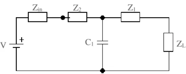
3.1.3 Mixed element structures formed with one capacitor and two UEs ... 24
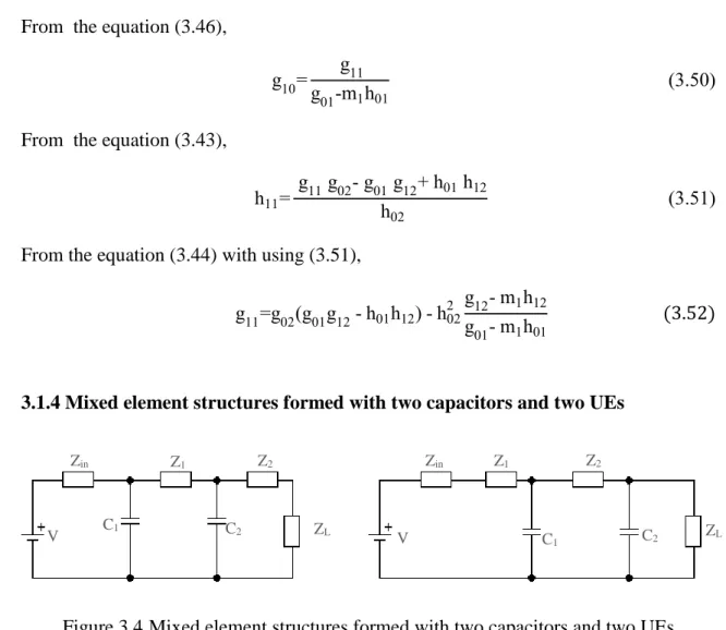
3.1.4 Mixed element structures formed with two capacitors and two UEs ... 26
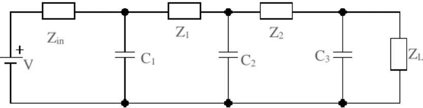
3.1.5 Mixed element structures formed with three capacitors and two UEs ... 29
3.2 Characteristic Impedance and Capacitance Calculations... 33
3.2.1 Characteristic impedance calculations of unit elements ... 33
3.2.2 Capacitance calculations ... 35
4. BROADBAND MATCHING NETWORKS ... 39
4.1 Line Segment Technique for a Single Matching Problem ... 40
4.2 Solution for Double Matching Problems ... 41
4.3 Parametric Representation of Brune Functions... 43
4.4 Real Frequency Matching with Scattering Parameters ... 45
5. EXAMPLES ... 48
5.1 Broadband Matching Network Formed with Mixed Element Structure ... 48
6. CONCLUSION ... 56
REFERENCES ... 57
CURRICULUM VITAE ... 59
APPENDIX A ... 60
A.1 Participation Certificate ... 60
APPENDIX B ... 61
B.1 Matlab Codes Main Program ... 61
B.2 Matlab Codes Error Calculation ... 66
B.3 Matlab Codes Last Column of g Matrix ... 69
B.4 Matlab Codes First Row of g Matrix ... 70
B.5 Matlab Codes Paraconjugate Calculations ... 71
B.6 Matlab Codes One Capacitor and One UE ... 71
B.7 Matlab Codes Two Capacitors and One UE ... 72
B.8 Matlab Codes One Capacitor and Two UEs ... 73
B.9 Matlab Codes Two Capacitors and Two UEs ... 74
i
ANALYSIS OF STRUCTURES FORMED WITH SHUNT CAPACITORS SEPERATED BY TRANSMISSION LINES
ABSTRACT
There are many works in literature about ladder networks containing inductors and capacitors. But usually it is not desired for the designed circuit to have inductors since they are heavy, bulky and available only for a limited range of values and are difficult to implement at microwave frequencies, they are approximated with distributed components. Richard’s transformation is used to convert lumped elements to transmission line sections.
Now consider a low-pass lumped ladder network. If the series inductors between the shunt capacitors are replaced with equal length transmission lines, a practically important mixed structure is obtained. Since the lengths of all the transmission lines are the same, these lines are called commensurate lines or unit elements (UE). It is very practical to fabricate this structure. If the transmission lines are quarter wavelength long, they are referred to as admittance inverters. These structures are useful especially for narrowband (<10%) bandpass and bandstop filters.
In this thesis, as opposed to the structures existing in the literature and explained above briefly, it is not necessary to have quarter wavelength transmission lines. So it is possible to design broadband circuits. Also the transmission lines separating the parallel capacitors are not redundant elements, they are used as circuit elements effective for the desired response. Additionaly if it is preferred not to have shunt capacitors, they can be replaced with open-ended stubs via Richard’s transformation. So the resultant circuit is extremely suitable for microstrip fabrication.
In this thesis, the analysis of the mentioned mixed structure has been performed first time in the literature in the following manner. The description of the structure by means of two frequency variables (one for shunt capacitors and one for transmission lines) has been
ii
detailed. Then broadband matching networks for military and commercial applications have been designed by using this practically important mixed structure via the algorithm that has been developed. In the algorithm, the explicit expressions for the coefficients of the descriptive two-variable polynomials in terms of the coefficients of the single variable boundary polynomials have been derived for various numbers of elements. These coefficient relations have been obtained first time in the literature. Since the lumped section contains only shunt capacitors (a degenerate network), it is impossible to use the two-variable polynomials to calculate the capacitor values. So a synthesis algorithm for the structure has been developed to be able to get the capacitor values from the two variable polynomials.
Normalized prototype circuits can be designed via the developed algorithm. So the prototype circuit can be denormalized via the frequency and impedance normalization numbers selected by the designer considering the interested frequency band and impedance level.
iii
İLETİM HATLARI İLE AYRILMIŞ PARALEL KONDANSATÖRLER İÇEREN YAPILARIN ANALİZİ
ÖZET
Bobin ve kondansatörlerden oluşan merdiven devreler hakkında literatürde birçok çalışma bulunmaktadır. Fakat genellikle, ağır ve büyük oldukları için, üretilebilecek değer aralıklarının sınırlı olması ve mikrodalga frekanslardaki üretim güçlüklerinden dolayı, tasarlanan devrelerde bobin olması istenmez dağıtılmış elemanlar (iletim hatları) ile yaklaşık olarak gerçeklenmeye çalışılırlar. Toplu elemanların dağıtılmış elemanlara çevrilmesinde Richards dönüşümü kullanılır.
Paralel bağlı kondansatörlerin arasındaki seri böbinleri, eşit uzunlukta iletim hatları ile değiştirelim. Bu iletim hatları Birim Eleman (BE) olarak isimlendirilir. Eğer hat parçalarının uzunluğu çeyrek dalga boyu olarak seçilirse admitans inverterleri elde edilir. Bu yapılar, özellikle dar bantlı (<10%) band geçiren ve band durduran filter olarak kullanılmaktadır.
Bu tezde, yukarıda kısaca açıklanan yapılardaki iletim hatlarının, literatürdekinin aksine, çeyrek dalga boyu uzunluğunda olma zorunluluğu yoktur. Bu sayede geniş bantlı devreler tasarlanabilmektedir. Ayrıca kondansatörler arasındaki iletim hatları sadece kondansatörleri ayıran, elemanlar olarak yer almayıp, devrenin istenen cevabı vermesi için devre elemanı olarak kullanılmaktadır. Eğer devrede toplu eleman (paralel kondansatör) olması istenmezse, Richards dönüşümü kullanılarak açık-uçlu hat parçaları ile değiştirilebilirler. Sonuç olarak elde edilen devre mikrostrip üretimi için son derece elverişli bir yapı olacaktır.
Bu tezde, yukarıda açıklanan devre yapısının literatürdeki ilk analizi yapılmıştır. Pratik açıdan çok önemli bu yapının iki-değişkenli tanımı detaylı olarak verilmiş, geliştirilen algoritma ile bu yapı kullanılarak bir çok askeri ve ticari uygulamada yer alabilecek genişbant empedans uyumlaştırma devresi tasarımları gerçekleştirilmiştir. Bu
iv
tasarımların yapılabilmesi için, devreyi tanımlayan iki-değişkenli polinomların katsayıları, tek-değişkenli sınır polinomlarının katsayıları kullanılarak hesaplanmıştır. Tüm bu katsayı ifadeleri, devredeki eleman sayısına yani devre derecesine bağlıdır. Devrede en fazla üç kondansatör ve iki hat parçası bulunduğunda katsayı ilişkileri elde edilebilmiştir. Literature bu katsayı ilişkileri kazandırılmıştır. Toplu eleman içeren kısım sadece paralel bağlı kondansatörlerden oluştuğu için (dejenere devre), algoritma sonucunda elde edilen iki-değişkenli polinomlar kullanılarak, kondansatör değerlerinin hesaplanması için yeni bir yaklaşım geliştirilmiştir.
Ayrıca, geliştirilen algoritma ile normalize edilmiş prototip uyumlaştırma devresi tasarımları yapılmaktadır. Dolayısıyla, tasarımcı tarafından, uygulamanın gerektirdiği frekans ve empedans değerlerine uygun normalizasyon sayıları seçilerek tasarlanan devrenin istenen frekans bölgesinde ve empedans seviyesinde çalışması sağlanabilmektedir.
v
ACKNOWLEDGEMENTS
People in their life may have some difficulties to reach their targets. These difficulties are sometimes so formidable without someone advices and guidance. Only the lucky ones have a patient and determined counsellor around them. I think, I am one of the lucky ones to have a supervisor Assoc. Prof. Metin Şengül. By the help of you, I can have the power and determination to finish the master thesis and continue my academic career.
Thanks Professor.
This thesis is supported by Kadir Has University Scientific Research Project, 2017- BAP-15
vi
LIST OF TABLES
vii
LIST OF FIGURES
Figure 2.1 Capacitor and transmission line equivalent…….………04
Figure 2.2 Inductor and transmission line equivalent…….………..…....04
Figure 2.3 Two port network……..………...………...………...05
Figure 2.4 Lumped element representation of a transmission line …….……...………..07
Figure 2.5 Two port network with waves ………...………...………..09
Figure 3.1. Mixed element structures formed with one capacitor and one UE...19
Figure 3.2 Mixed element structures formed with two capacitors and one UE...22
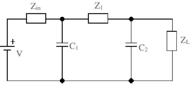
Figure 3.3 Mixed element structures formed with one capacitor and two UEs...24
Figure 3.4Mixed element structures formed with two capacitors and two UEs...26
Figure 3.5 Mixed element structures formed with three capacitors and two UEs...30
Figure 5.1 Designed broadband matching network………...………...51
1
1. INTRODUCTION
The broadband matching problems are solved by using distributed elements in high frequency applications instead of using lumped components. Because of the implementation problems for lumped components in circuits, the distributed elements are prefered for the circuit designs in microwave frequencies. The lumped elements are used as the equivalence of the distributed components according to the physical size. To receive better performance, ideal lumped and distributed components can be utilized together to form a lossless matching networks with mixed, lumped and distributed components by the help of the Richards transformation.
In this thesis, the research is based on the analysis of the lossless ladder circuits which ones are formed with parallel capacitors separated with the unit elements. Inductors aren’t used in this design because of the size and weight. This component causes implementation problems in microwave filters or broadband matching networks. The restrictions about bandwidth in microwave circuits design is another reason for the useless of the inductor. In literature, there are lots of studies about the ladder networks which involve only distributed components, lumped components or both of them. (Yarman, 2008) is a study for ladder networks with only lumped elements. (Aksen, 1994) is a study for low-pass ladder networks which contains inductor and capacitor as lumped elements and the lumped elements are separated by Unit Elements. This study is based on the coefficients of the variables up to 5 components. (Sertbaş, 1997) is an analysis according to the high pass, bandpass and stopband networks which contains distributed components. (Şengül, 2006) is an examination to circuit design which are formed due to the structures and rules of the other three researches.
(Şengül, 2009) is about the mixed elements ladder networks which have the same responses with the distributed components. In order to form mixed element networks,
2
Richards Transformation (λ=tanh 𝛽𝑙) is used to transform the lumped elements to the distributed elements and with the help of the Kuroda identities (Kurokawa, 1965), the way of placement of the transmission lines can be changed .
A low pass ladder network can be formed with the lumped elements and there are transmission lines between these lumped elements. The transmission lines are replaced with the inductors. The resistances can be the first element and the last of these circuits. These transmission lines have quarter-wavelength long. These structures useful for narrowband, bandpass and bandstop filters. In this thesis, all of the wavelengths are equal and the value of the quarter wavelength length of the transmission line is not an indispensable condition to develop wideband circuit designs. These transmission lines are used like a circuit components to get requested response of the circuit. In addition of all these option, the capacitor can be replaced with the open circuit transmission lines with the help of the Richards transformation.
After explanation of the circuit structure, the analysis of these ladder networks with mixed elements. The approach is to explain the mixed and distributed elements in lossless two port network. With the help of the Richards transformation, the multivariable synthesis procedure can be used to generalize the approach due to the mixed lumped and distributed elements. The Richards variable λ is identified for distributed elements and the frequency variable p is identified for lumped elements. To get the values of capacitor and transmission line, the coefficients of the two variable g(p,𝜆) and h(p,λ) polynomials must be calculated with the restricted one variable polynomials g(p), h(p) and g(λ), h(λ). The number of the components are started from the 2 and up to 5 in this thesis. The capacitor is the only one to use in this design so there is a need to find a new way to calculate the values of the capacitors. With the selection of proper value for normalization, the circuit can be operated with desired value of frequency and impedance.
3
2. LUMPED AND DISTRIBUTED COMPONENTS
Growing needs of people causes important and significant developments in communication and circuit technology, especially in MIC technology. Naturally this development face with difficulties about design of networks by using lumped and distributed components. Lumped and distributed components are utilized mostly in RF and microwave engineering due to their frequency parameters. While engineers fabricate these networks according to needs, their main wish is minimization of the loss power or voltage through the transmission lines used as a way for conveying the voltage or powers from the generator to the load components. As you can see, best transmission lines are the lossless ones for designers.
2.1 Transmission Line Components
Lumped and distributed components are used for solving filter and broadband matching distress in RF and microwave circuits. These lumped components are electrical components acted as inductor, capacitor or resistor in low frequencies mostly in RF designs. They use in low frequencies because of the restriction of the small dimension (Ld). This dimension must be less than the ratio of wavelength (ƴ ) at specific frequency.
The wavelength (ƴ ) is calculated by dividing the speed of light to given frequency. There is no general acceptance in literature so ƴ/20 or ƴ/10 can be accepted. The restriction is that the Ld must be less than ƴ /20or ƴ/10. If the circuit components respond this rules, the
network will be called lumped otherwise distributed network. The lumped elements are used in RF owing to some advantages in low frequencies. Some have smaller sizes and smaller coupling, amplitude, phase changes.
One of the transmission line components is the distributed components which are used in high frequencies owing to implementation problem of lumped elements in high frequencies. One of the problem is caused by inductor, inductors don’t allow the current
4
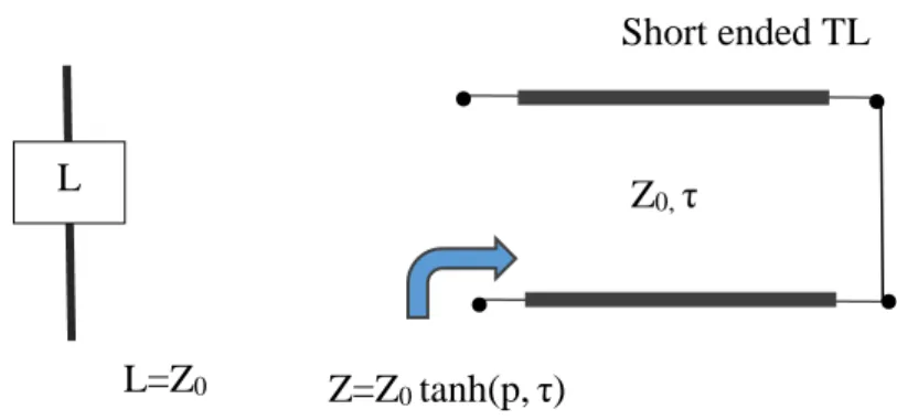
to pass through so it becomes an open-circuit in high frequency. The other one is capacitor. The capacitor becomes a short-circuit so voltage can’t be measured on its part. The situation is useless for matching and filter design in microwave circuits. According this situation, distributed components are used instead of lumped elements with transmission lines in distributed circuit. The inductor is converted to the short ended transmission line and the capacitor is converted to open-ended transmission line. The transmission line which one has impedance and delay of transmission line (τ) is the last member of the distributed elements. In Figure 2.1 show the transformation a lump circuit to distributed one. By this way, designers don’t have to deal with the complex frequency. The calculation can be done with using impedance, length of the circuit elements values and the others.
Figure 2.1 Capacitor and transmission line equivalent
Figure 2.2 Inductor and transmission line equivalent C Z=Z0 coth(p,τ) Open ended TL C=1/Z0 Z0, τ L Z=Z0 tanh(p,τ) Short ended TL L=Z0 Z0, τ
5 pis the complex frequency.
p= α + jw (2.1) τ is the delay of transmission line. Z is the impedance. Z0 is the characteristic impedance.
ƴ is the wavelength. α is the attenuation constant.
Although, there is a solution for the calculations in design circuits at high frequencies by the help of the distributed components. The shunt capacitor causes problems in circuits. Because of this problems, Richards transformation (Richards, 1948) approach is used for transforming transcendental functions of the distributed networks to rational functions. By the help of the Richards transformation (λ= tanh(pτ)), the mixed lumped and distributed networks become very important for the development in microwave technology. Richards approach provides multivariable synthesis process where the Richard value λ for the distributed elements and frequency variable p for the lumped elements.
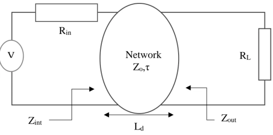
Figure 2.3 Two-port network
Zint is the input impedance. Zout is the output impedance. Ld is the length of transmission
unit. Z0 is the characteristic impedance of transmission line. V represents the source of
voltage. Rin is the generater resistance. RL is the load resistance in the load of the network.
Rin RL V Zint Zout Network Zo,τ Ld
6
The input impedance is calculated like this according to the wave which is provided from the source, follows the transmission line to the load. By using these parameters, the input impedance can be calculated.
λ=tanh(pτ) (2.2) Zint=Z0 RL +λ Z0 Z0 +λRL (2.3) Zint=Z0 R0 L + tanh (pτ) Z0 Z0 + tanh (pτ) RL (2.4) The output impedance can be calculated.
Zout=Z0 Rin + tanh (pτ) Z0 Z0 + tanh (pτ) Rin (2.5) or Zout=Z0 Rin +λ Z0 Z0 +λRin (2.6)
The open circuit TL is formulated in condition of the value of the terminated impedance (ZL) is infinity. The formulation shows the calculation:
Zint= lim ZL→∞Z0 ZL +λ Z0 Z0 +λZL =Z0 (2.7) The short circuit TL is formulated with the condition of the value of the terminated impedance (ZL) is zero. The formulation shows the calculation:
Zint= lim ZL→0Z0
ZL +λ Z0
Z0 +λZL=λZ0 (2.8)
2.2 Transmission Line as a Circuit Elements
Transmission line can be explained in electrical parameter. These electrical parameters are characteristic impedance (Zo), phase constant (β), attenuation constant (α), physical
length (Ld) and propagation value (¥). By the help of these parameters, parameters can be
7
f is the operation frequency in circuits. ƴ is the wavelength of the transmission line.
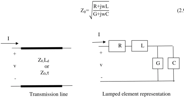
A transmission line analysis can be done with calculating the impedance of a circuit which one is formed with resistance, inductor in serial and admittance and capacitor in parallel like in Figure 2.4.
For a lossy transmission line, the formulation of characteristic impedance of line will be;
Z0=√
R+jwL
G+jwC (2.9)
Figure 2.4 Lumped element representation of a transmission line
The calculation of the propagation constant is for lossy transmission line.
The phase constant is represented with β. G is the conductance. Ld is the physical length
of the transmission line. Pv is the phase velocity. ϕ is the phase delay measured in radians.
¥ =√(R+jwL)(G+jwC) (2.10) or
¥=α+jβ (2.11) For a lossless transmission line, R and G are 0 and the formulation of characteristic impedance of line will be:
R L G C V i V + v - + v - I I Z0,Ld or Z0,τ
Lumped element representation Transmission line
8 𝑍0 = √L
C (2.12) The propagation constant is formulated as:
¥=√LC (2.13)
2.3 The Utilization of Transmission Lines in Two Port Networks
Impedance and admittance methods are used to calculate the efficiency of gain power transmissions of circuits in low frequencies. These parameters are not useful for high frequencies because they require voltage and current which ones are calculated with the open – short methods (like Thevenin). In high frequencies, these methods are impractical so a new approach is required like scattering parameters. The scattering parameters are calculated according to the flowed waves with forward and backward directions in transmission lines.
The sign of the applied wave to the network show as a and the reflected wave show as b in input and output port of circuits like in Figure 2.5. If Z0 (the characteristic impedance
of transmission line ) is equal to the RL ( the load resistance ), the reflection is not occured
from the load resistance. That means the applied power from the source is entirely dissipated in RL. In the condition of Z0≠RL, the some amount of the power will dissipate
in transmission line or the reflecion wave is occured from the RL. The efficiency of gain
power transmission is not provided as desired.
As seen in Figure 2.5, the normalized applied voltage wave (incident wave) is a1 in
forward direction at the first port and the reflected volage wave b1 is backward direciton
in the first port. The a2 is the normalized applied voltage wave and the b2 is the reflected
9
Figure 2.5 Two − port network with waves
The calculations of the normalized incident and reflected waves are a and b in input and output ports. They are defined as:
a1= (V1+Rin Iint) 2√Rin (2.14) b1=(V2-RinIint) 2√Rin (2.15) a2= (V1+RLI0) 2√RL (2.16) b2= (V2-RLI0) 2√RL (2.17)
The value of the total voltage Vn and total curent In are defined in two-port. n representes
the port number.
V1=(a1+b1)√Rin (2.18) Network Z0 τ b1 a1 b2 a2 Zint Zout V Rin RL l=0 l=z + V1 - + V2 -
10 I1= a1-b1 √Rin (2.19) V2=(a2+b2)√RL (2.20)
Due to these waves parameters, the reflection parameters of input, outport ports and load can be calculated
I2=
a2-b2
√RL
(2.21)
Sint represents the input reflection coefficient. Sint=
b1 a1=
Zint - Rin
Zint + Rin (2.22)
Sout represents the output reflection coefficient. Sout=
b2 a2=
Zout-ZL
Zout+ZL (2.23)
SL represents the load reflection coefficient.
SL=
ZL-Zout
ZL+Zout (2.24)
Sin representes the reflection coefficient from the generater:
Sin=
Zin-1
Zin+1 (2.25)
The reflected power can be calculated by taking square of the reflection coefficient. The reflected power is defined as 𝑃𝑅.
PR=b2 (2.26) The incident power can be calculated with taking square of the incident coefficient.
The incident power is defined as 𝑃𝑖.
Pi=a2 (2.27) The total power in ports can be calculated with difference of the power incident wave and power reflected wave. 𝑃1 is representation of the power in port 1.
11
P1=Pi-PR=a12-b12 (2.28)
P2 is the total power in port 2.
P2 = Pi-PR=a22-b22 (2.29)
The total power of the system is calculated with the summation of the dissipated total powers in two ports. PT represents the total power of the network.
PT = P1 + P2 (2.30)
Transducer power gain of the two port is defined as:
TPG=1-|SL|2 (2.31)
2.4 The Definition of Scattering Parameters and Scattering Matrix
Scattering parameter (Fettweis, 1982) for the explanations of power transfer is pratical and useful tool for networks work at high frequecies. This method is used for finite values at output and input of the network. The tools use open circuits to find values of voltage and current of the network. Another difference between scattering parameter and others are structure of values in networks. In scattering parameters, the waves of voltage and current are utilized to calculate the efficiency of the network.
Previous Seciton 2.3 is about the structure of waves. In this sections, these waves are used to form scattering parameters. In Figure 2.5, the parameters a and b are used for the definition of the scattering parameters. Scattering parameters are the values of the scattering matrix for two port network as:
b= [bb1 2] , a= [ a1 a2] , S= [ S11 S12 S21 S22] (2.32)
S represent the scattering matrix, Sij represent the values of the scattering parameter, i is
for the number of the matrix raw, j is for the number of the coloumn of the matrix.
The relations between the scattering matrix and waves are defined as in below.
12
If a2 is 0, there is no reflection wave from the terminated load resistance (ZL) because of
the equal match between ZL and Zout.
Input reflection is:
S11=
b1
a1 (2.33)
Transducer power gain from input to outport port is: S21=b2
a1 (2.34) If a1 is 0, there is an equal match between Zint and Rint.
Output reflection is:
S22=
b2
a2 (2.35)
Transducer power gain in reverse direction is: S12=
b1
a2 (2.36)
The formula of dissipated power in two port is written in equation (2.37). This formula can be written with the scattering parameter like:
Pd=a*Ta(I-S*TS) (2.37)
I represent the identity matrix, * is the transposed conjugate of a matrix. If scattering matrix is unitary means, Pd is always greater or equal to the zero.
For lossless network,
I-S*TS=0 S*TS=I (2.38) The equation (2.32) is a link for scattering parameters with each other.
S11*S11+S21*S21=1 (2.39)
13
S12*S11+S21S22* =0 (2.41)
S21*S22+S12S11=0 (2.42)
If the network is reciprocal, scattering matrix is symmetrical. Symmetrical means the transposed of a network is equal to its own matrix. For a lossless network, the transmittance of forward and reverse direction are equal each other
ST=S (2.43)
S21=S12 (2.44)
Scattering transfer matrix (T) is used for cascade connections instead of only scattering matrix (Fetweis, 1970). The relations of normalized waves with the trasfer matrix parameters according this formula:
[ba1 1] =T [ a2 b2], T= [ T11 T12 T21 T22] (2.45)
The transfer scattering parameters are: T11= -detS S21 T21 =-S22 S21 T12= S11 S21 T22= 1 S21 (2.46)
Reciprocal scattering matrix causes the result of determinant of transfer scattering matrix to be 1 (det T =1).
2.5 Canonic Representation of Scattering and Scattering Transfer Matrix
f, g and h are three canonic polynomials and these parameters are for the explanation of the scattering matrix parameters and the scattering transfer matrix. As seen in the formulas of scattering matrix and transfer matrix:
S= [ h g σf* g f g -σh* g ] T= [ σg* f h f σh* f g f ] (2.47)
f* means f(-p) where p is the complex frequency (p=α+jβ). These are the properties of the
14
f(p), h(p) and g(p) are real polynomials in complex frequency p. g is strictly Hurwitz polynomial (Fettweis, 1982). f, g and h parameters have a relation according to this formula:
g g*=hh*+ff* (2.48) σ is the constant 1 or -1.
Supposing the two-port network is resiprocal, the value of the f polynomial can be even or odd. This situation effects the value of σ canstant 1 or -1 with f is even and f is odd. With this properties the formula of (2.48) can be changed to this:
gg*=hh*+σf2 (2.49)
According to another role, degree of g polynomial is equal or larger than the degree of h polynomial and the degree of polynomial f. The transmission zeros at infinity is calculated with taking difference of the degree of polynomial g and the degree of polynomial f.. The directions are S21 and S12 scattering parameters and the calculation
will be done with 3 canonic polynomials (f, g, h). Due to the (2.49) formula, S12 is equal
to f/g and S21 is equal to f*/g. With the (2.49), this formula can be written:
ff*
g2 =
gg*-hh*
g2 (2.50)
If ff* is a real even polynomial, locations of zeros are symmetry with the jw axis. By the
help of the g’s strictly Hurwits property, any cancellation can not be occured in ff* in the
closed right half plane. Real part of p is equal to zero or a possitive number. Due to the these conditions, the number of finite transmission zeros can be received from the degree of f and the infinity transmission zeros can be received with difference of deg g and deg f. Number of the finite and infinity transmission zeros are determined from the degree of g polynomial on condition of 0 ≤ Re(p).
The input impedance of Figure 2.3 with output is terminated with a resistance (Z0)
can be calculated with polynomials. Zint= 1+S11 1-S11 = g+h g-h= n d (2.51)
15
By calculating the even part of the Zint, all of the transmission zeros can be identified.
Even part of the Zint is calculated as:
Zint= 1 2(Zint+Zint*)= 1 2( n d+ n* d*) = 1 2( nd*+n*d dd* ) = ff* (g-h)(g*+h*) (2.52)
Because of the numerator and denominator terms in last part of the formula, the jw zeros are eliminated. The 0.5(nd*+n*d) is equal to the ff* and the finite transmission
zeros can be found in this part. Under this situation, all of the transmission zeros can be determined by equation (3.4).
16
3.TWO VARIABLE CHARACTERIZATION OF MIXED
STRUCTURES
For implementation of the lumped and distributed components together in cascaded lossless two port (Şengül, 2010), the two variable characterization method is needed. By the help of the Richard’s transformation, one of the variable is Richards variable λ and the other one is the complex frequency variable p. Lumped sections can be formed according to the p and the distributed sections can be formed due to Richards variable. If these two variable are assumed indipendent variable with each other, the implementation of the lumped and distributed components can be achieved by the using multivariable methods (Şengül, 2009).
The relation between the f, g, h two variable polynomials with scatter parameters is shown as: S(p,λ)= 1 g(p,λ)[ h(p,λ) σf(p,λ) f(p,λ) -σh(p,λ)] (3.1) S11= h(p,λ) g(p,λ), S12= σf(p,λ) g(p,λ) , S21= f(p,λ) g(p,λ), S22= -σh(p,λ) g(p,λ) (3.2) Scatttering parameters in (3.1) are formed with one variable scattering parameters s(p) and s(λ). S(p) and S(λ) are the explanation of the scattering parameters of lumped (p) and distributed (λ) sections. In a project, the number of the components are the determination of transmission zeros in networks.
17
g(p,λ) is a scattering Hurtwitz polynomial with two variable. The formula of g(p,λ) is formed with the coefficients:
g(p,λ)= ∑ ∑ gijpiλj Np j=0 Nλ i=0 (3.3)
Variable p is for the lumped and λ is for the distributed sections. Nλ is the number of the
the distributed elements (Unit Element) and Np is the number of the lumped elements in
cascaded network.
Another representation of the g(p,λ) is for the thesis which has the first row for the distributed coefficients and the last column is for the coefficients of lumped. The others are unknown coefficients whichs are solved with the algorithm improved in this thesis to find accurate values of capacitors and impedance of UEs:
g(p,λ)=pTM gλ (3.4) Mg= [ g00 ⋯ g0N λ ⋮ ⋱ ⋮ gN p0 ⋯ gNpNλ ] (3.5)
In (2.49) formula, G(p,λ)=gg* means multiplication of the g function with pozitif variable
(p,λ) and the same function with negative variable (-p,-λ). The degree of result function can be used to identify the finite and infinity transmission zeros of the network.
g(p,λ) is one of the polynomial used in equation (3.4). The first row is for the distributed coefficients and the last column is for the coefficients of the lumped elements. These are the known coefficients in this thesis. There are other known coefficients whichs values are zero in matrix. All accept these known coefficients are the unkown coefficients and can be calculated with using algorithm identificated in this thesis.
The formulation of the zeros coefficients:
18 Mh= [ h00 ⋯ h0Nλ ⋮ ⋱ ⋮ hNp0 ⋯ hNpNλ ] (3.7)
In (2.48) formula, H(p,λ)=hh* means multiplication of the h function with pozitif variable
(p,λ) and the same function with negative variable (-p,-λ).
h(p,λ) is one of the polynomial used in equation (2.48). The first row is for the distributed coefficients and the last column is for the coefficients of the lumped elements. These are the known coefficients in this thesis. There are other known coefficients whichs values are zero in matrix. Accept these known coefficients, the others are the unknown coefficients calculated by using algorithm identificated in this thesis.
If a two-port network has UEs in cascaded mode, the f(p,λ) is defined as: f(p,λ)=pk1 (1-λ2 ) u 2 ⁄ (3.8) In formula (3.8), k1 is the number of transmission zeros at dc and it is equal 0 in this thesis because there is no serial capacitor and paralel inductor components in network. U represents the number of cascaded UEs in networks.
For k1 =0, f(p,λ)=pk1 (1-λ2) u 2 ⁄ =f(p)f(λ) (3.9) In this thesis, g00=1, h00=0 and f00=1 are chosen for the same input and output
normilization for f00=0k2(1-02)u/2 no matter value of the u in this condition, the answer is
always 1.
In (2.48) formula, F(p,λ)=ff* means multiplication of the f function with pozitif variable
f(p,λ) and the same function with negative variable f(-p,-λ). F function is used for the identification of the finite transmission zeros in network.
In low pass ladder, the number of k1 is equal zero at infinity because there are no capacitior in series and inductor in paralel at the circuits.
19
3.1 Analysis of Mixed Element Structures
In this thesis, the low pass ladders have paralel capacitors separated with unit elements. The capacitors are the lumped components (p) and the unit elements (λ) with impedance (Z0) and transmission delay (τ) are distributed elements. The aim of this algorithm to find
the unknown coefficients in
M
handM
g.
By using G(p,f) and H(p,f), the proper value ofcapacitors and unit elements can be calculated for broadband matching examples. The total degree (Np+Nλ) of the networks are 2 to 5 in this thesis.
3.1.1 Mixed element structures formed with one capacitor and one UE
Figure 3.1 Mixed element structures formed with one capacitor and one unit element
This network has one capacitor (Np=1) and one unit element (Nλ=1). According to
equation (2.48), two variable functions f, g, h are shown as:
For u=1 and f(p)=1,
f(p,λ)=pk1 (1-λ2 ) u 2 ⁄ =p0 (1-λ2 ) 1 2 ⁄ (3.10) For (3.10), F(p,λ)= f(p,λ)f(-p,-λ)= (1-λ2) (3.11) H(p, λ)=h(p, λ)h(-p,-λ) (3.12) h(p, λ)=0+h01λ+h10p+h11p λ (3.13) ZL C1 Z1 Zin ZL Z1 Zin C1 V V
20
The matrix of
M
h has 2×2 dimensions and h00 is 0. According to the equation (3.8), thematrix is:
Mh= [h00 h01
h10 h11] (3.14)
The known parameters are h00, h01, ℎ11 and the unknown coefficient is h10. The
boundaries are the last column for distributed and the first row for lumped elements. G(p, λ)=g(p, λ)g(-p,-λ) (3.15) The matrix of
M
g has 2×2 dimensions and g00 is 1. According to the equation (3.5), thematrix is:
Mg= [
g00 g01
g10 g11] (3.16) The known parameters are g00, g01, g11 and the unknown coefficient is g10. The boundaries are the last column for distributed and the first row for lumped elements.
G(p, λ)= H(p, λ)+ F(p,λ) (3.17) According to these properties and explanation about F, G, H polynomials. The unknown coefficients of G and H can be calculated by algorithm which one is the main goal of the thesis.
G(p, λ) - H(p, λ) - F(p,λ)=0 (3.18) The equations are formed with using Matlab according to the result of equation (3.18). The result is the main equation which has parameters like powered λ and p (disjoint p,λ and adjacents pλ onces) and powered coefficients. This equation is needed to be paranthesized due to the same powered λ for getting new equations which ones have only parameters contains powered p and powered coefficients. Finally, this equation is paranthesized according to the same powered p and get equations containing powered coefficients or parameters of
M
hand M
g. These last equations are all equal to zero. Bythe help of these equations, the unknown coefficients can be calculated.
The equations are provided with using Matlab. These equations are: g112 - h
11
21 g012 - h 01 2 =0 (3.20) g11- g10g01+ h01h10=0 (3.21) g102 - h 10 2 =0 (3.22)
The unknown coefficients g10 and h10 are calculated with these equations.
From the equation (3.22),
g10=|h10|→ m1=
h10
g10 (3.23) From the equation (3.19),
g11=|h11|→ m2=h11
g11 (3.24) From the equation (3.21),
g10= g11
g01-mh01 (3.25) If m2 is equal to 1, the first component is capacitor. If m2 is equal to -1, the first component is unit element. The constant value of m1 is -1.
3.1.2 Mixed element structures formed with two capacitors and one UE
This network has two capacitors (Np=2) and one unit element (Nλ=1). The matrix of Mh
has 3×2 dimensions and h00 is 0. According to the equation (3.7), the matrix is:
Mh=[
0 h01 h10 h11
0 h21
] (3.26)
The known parameters are h00, h01, h11, h21, h20 and the unknown coefficient is h10. The boundaries are the last column for distributed and the first raw for lumped elements.
22
The matrix of Mg has 3×2 dimensions and g20 is 0 and g00 is1.
Mg=[
1 g01 g10 g11 0 g12
] (3.27)
The known parameters are g00, g01, g11, g12 and the unknown coefficient is g10. The boundaries are the last column for distributed and the first raw for lumped elements.
Figure 3.2 Mixed element structures formed with two capacitors and one UE According to these properties and explanation about F, G, H polynomials.The unknown coefficients of G and H can be calculated with algorithm.
The equations are formed with using matlab according to the resut of this equation (3.18). The result is the main equation which has parameters like powered λ and p ( disjoint p, λ and adjacents pλ onces) and powered coefficients. This equation is needed to be paranthesized due to the same powered λ for getting new equations which ones have only parameters contains powered p and powered coefficients. Finally, this equation is paranthesized according to the same powered p and get equations contain powered coefficients or parameters of Mh
and
Mg. These last equations are all equal to zero. Bythe help of these equations, the unknown coefficients can be calculated.
These equations are provided with using matlab. These equations are: g012 − h 01 2 =1 (3.28) g212 − h 21 2 = 0 (3.29) ZL Z1 Zin C1 C2 V
23 g202 − h 20 2 = 0 (3.30) g102 − h 10 2 − 2(g20) = 0 (3.31) g112 − h 11 2 − 2(g01g21 − h01h21)=0 (3.32) g11g20− h11h20− g10g21+ h10h21=0 (3.33) g11− g10g01+ h01h10=0 (3.34) The unknown parameters g10 and h10 are calculated with these equations.
For this structure, m1= -1, m2= -1.
From the equation (3.31):
g10=|h10|→m1=
h10
g10 (3.35) From the equation (3.29):
g21=|h21|→ m2=
h21
g21 (3.36) From the equation (3.34):
g10= g11
g01− m1h01 (3.37)
From the equation (3.31):
24
3.1.3 Mixed element structures formed with one capacitor and two UEs
Figure 3.3 Mixed element structures formed with one capacitor and two UEs
This network has one capacitor (Np=1) and two Unit Elements (Nλ=2). The matrix of Mh
has 2×3 dimensions and h00 is 0. According to the equation (3.12), the matrix is:
Mh= [h0 h01 h02
10 h11 h12] (3.39)
The known parameters are h00, h01, h02, h12, and the unknown coefficients are h10, h11. The boundaries are the last column for distributed and the first row for lumped elements.
The matrix of
M
ghas 3×2 dimensions and g00 is 1.Mg= [
1 g01 g02
g10 g11 g12] (3.40) The known parameters are g00, g01, g02, g12 and the unknown coefficients are g10 , g11. The boundaries are the last column for distributed and the first row for lumped elements.
According to these properties and explanation about F, G, H polynomials. The unknown coefficients of G and H can be calculated with algorithm.
The equations are formed with using Matlab according to the resut of this equation (3.18). The result is the main equation which has parameters like powered λ and p (disjoint p,λ and adjacents pλ onces) and powered coefficients. This equation is needed to be paranthesized due to the same powered λ for getting new equations which ones have only parameters contains powered p and powered coefficients. Finally, this equation is paranthesized according to the same powered p and get equations contain powered
ZL Z1 Z2 Zin C1 V
25
coefficients or coefficients of Mh
and
Mg . These last equations are all equal to zero. Bythe help of these equations, the unknown coefficients can be calculated.
These equations are provided by using Matlab. These equations are: g122 − h 12 2 = 0 (3.41) g022 − h 02 3 =0 (3.42) g11g02− h11h02− g01g12+ h01h12=0 (3.43) g112 − h 11 2 − 2(g12g10 − h12h10)= 0 (3.44) g012 − h 01 2 − 2g02=2 (3.45) g11− g10g01+ h01h10=0 (3.46) g102 − h 10 2 =0 (3.47)
For this structure, m1= -1, m2= +1.
The unknown parameters g11, g10, h11 and h10 are calculated by these equations.
From the equation (3.47):
g10=|h10|→m1=hg10 10
(3.48) From the equation (3.41),
g12=|h12|→m2=h12
26 From the equation (3.46),
g10= g11
g01-m1h01 (3.50)
From the equation (3.43),
h11= g11 g02- g01 g12+ h01 h12 h02
(3.51) From the equation (3.44) with using (3.51),
g11=g02(g01g12 - h01h12) - h022
g12- m1h12
g01- m1h01 (3.52)
3.1.4 Mixed element structures formed with two capacitors and two UEs
Figure 3.4Mixed element structures formed with two capacitors and two UEs This network has two capacitors (Np=2) and two unit elements (Nλ=2). The matrix of
M
hhas 3×3 dimensions and h00 is 0. According to the equation (3.8), the matrix is:
𝑀ℎ = [
0 h01 h02
h10 h11 h12
0 h21 h22
] (3.53)
The known parameters are h00, h01, h02, h12, h22, h20 and the unknown coefficients are
h10, h11, h21. The boundaries are the last column for distributed and the first row for
lumped elements.
The matrix of
M
ghas 3×3 dimensions and g20 is 0 and g00 is 1.Mg= [ 1 g01 g02 g10 g11 g12 0 g21 g22 ] (3.54) ZL ZL Z1 Z2 Z1 Z2 Zin Zin V C1 C2 V C1 C2
27
The known parameters are g00, g01, g02, g12 ,g22, g20 and the unknown coefficients are g10, g11, g21. The boundaries are the last column for distributed and the first row for lumped elements.
According to these properties and explanation about F, G, H polynomials. The unknown coefficients of G and H can be calculated with algorithm.
The equations are formed with using Matlab according to the resut of this equation (3.18). The result is the main equation which has parameters like powered λ and p (disjoint p, λ and adjacents pλ onces) and powered coefficients. This equation is needed to be paranthesized due to the same powered λ for getting new equations which ones have only parameters contains powered p and powered coefficients. Finally, this equation is paranthesized according to the same powered p and get equations contain powered coefficients or coefficients of Mh
and
Mg. These last equations are all equal to zero. Bythe help of these equations, the unknown coefficients can be calculated.
These equations are provided by using Matlab. These equations are: g102 − h 10 2 =0 (3.55) g11− g10g01+ h01h10=0 (3.56) g21g10− h21h10= 0 (3.57) g012 − h 01 2 − 2g02=2 (3.58) g112 - h112 -2(g12g10 - g22-h12h10+g01g21 - h01h21)=0 (3.59) g212 − h 21 2 =0 (3.60)
28 g11g02− h11h02− g01g12+ h01h12=0 (3.61) g11g22− h11h22− g21g12+ h21h12=0 (3.62) g022 − h 02 2 =1 (3.63) g122 − h 12 2 − 2(g02g22 − h02h22)=0 (3.64) g222 − h 22 2 =0 (3.65)
The unknown parameters g10, g11, g21 and h10, h11, h21 are calculated with these
equations.
From the equation (3.55),
g10=|h10|→m1=h10
g10 (3.66) From the equation (3.65),
g22=|h22|→m2=h22
g22 (3.67) From the equation (3.60),
g21=|h21|→m3=h21
g21 (3.68) From the equation (3.57),
m1 = m3 (3.69)
From the equation (3.56),
g10= g11
29 From the equation (3.61),
h11= g11 g02- g01 g12+ h01 h12
h02 (3.71) From the equation (3.56),
g21= g11 g22 - h11 h22
g12 - m1h12 (3.72)
From the equation (3.59) with using (3.72),
g11=g02(g01g12- h01h12) - h022 g12- m1h12 g01- m1h01+h02 2 (g01- m1h01)( g02h22 h02 - g22) g12- m1h12 (3.73)
For this structure, 𝑚1 = −1.
If 𝑚2 is equal to -1, the first component is capacitor.
If 𝑚2 is equal to 1, the first component is Unit Element.
3.1.5 Mixed element structures formed with three capacitors and two UEs
This network has three capacitors (Np=3) and two unit elements (Nλ=2). The matrix of
M
h has 4×3 dimensions and h00 is 0. According to the equation (3.12), the matrix is:Mh= [ 0 h01 h02 h10 h11 h12 0 h21 h22 0 0 h32 ] (3.74)
The known parameters are h00, h01, h02, h12, h22, h20, h32, h30, h31 and the unknown coefficients are h10, h11, h21. The boundaries are the last column for distributed and the first row for lumped elements.
30
Figure 3.5 Low order structure formed with three capacitors and two UEs
The matrix of
M
ghas 4×3 dimensions and g20, g30, g31 are 0 and g00 is 1.𝑀g
=
[ 1 g01 g02 g10 g11 g12 0 g21 g22 0 0 g32](3.75)
According to these properties and explanation about F, G, H polynomials. The unknown coefficients of G and H can be calculated by algorithm.
The equations are formed with using Matlab according to the resut of this equation (3.18). The result is the main equation which has parameters like powered λ and p (disjoint p, λ and adjacents pλ onces) and powered coefficients. This equation is needed to be paranthesized due to the same powered λ for getting new equations which ones have only parameters contains powered p and powered coefficients. Finally, this equation is paranthesized according to the same powered p and get equations contain powered coefficients or parameters of
M
hand M
g. These last equations are all equal to zero. Bythe help of these equations, the unknown coefficients can be calculated.
These equations are provided with using Matlab. These equations are:
g322 − h322 =0 (3.76) g222 −h222 − 2(g12g32− h12h32) = 0 (3.77) g122 −h122 − 2(g02g22− h02h22) = 0 (3.78) C2 C3 C1 Z1 Z2 Zin ZL V
31 g022 − h 02 2 =1 (3.79) g21g32− h21h32= 0 (3.80) g11g22− h11h22− g01g32+ h01h32 − g12g21+ h12h21=0 (3.81) g11g02− h11h02− g01g12+ h01h12=0 (3.82) g212 −h212 + 2(g10g32− h10h32) = 0 (3.83) g112 − h 11 2 + 2( g22− g12g10 + h12h10− g01g21 + h01h21)=0 (3.84) g012 − h 01 2 − 2g02=2 (3.85) g21g10− h21h10= 0 (3.86) g11− g10g01+ h01h10=0 (3.87) g102 − h 10 2 =0 (3.88)
For this situation, 𝑚1 = −1 𝑎𝑛𝑑 𝑚2 = −1.
From the equation (3.88):
g10=m1|h10|→m1=h10
g10 (3.89) From the equation (3.89):
32 From the equation (3.76):
g32=|h32|→m2=
h32
g32 (3.91) From the equation (3.91):
h32= m2 g32 (3.92)
From the equation (3.86):
g21=|h21|→m1=
h21
g21 (3.93) From the equation (3.93):
h21= m1 g21 (3.94) From the equation (3.80-86):
m1 = m2 (3.95)
From the equation (3.87):
g10= g11
g01− m1h01 (3.96)
From the equation (3.82):
h11= g11 g02− g01 g12+ h01 h12 h02
(3.97) From the equation (3.81):
g21= g11 g22− h11 h22 − g01g32+ h01h32
g12− m1h12 (3.98)
From the equation (3.84, 3.97, 3.98):
g11=g02(g01g12− h01h12) − h022 g12− m1h12 g01− m1h01+h02 2 (g01− m1h01)( g02h22 h02 − g22) g12− m1h12 (3.99) The order of the components are parallel capacitor, unit element, parallel capacitor, unit element and parallel capacitor, unit element in networks.
33
3.2 Characteristic Impedance and Capacitance Calculations
After the calculation of the unknown coefficients of g and h polynomials, the value of the cascaded lossless commensurate lines (Şengül, 2008) and the value of the capacitors are calculated due to the scattering transfer parameters.
3.2.1 Characteristic impedance calculations of unit elements
The realization problem of the lumped components in circuits with using microwave frequencies cause needs to use another approach. Distributed components are the solution for this problem. With the Richards transformation, distributed components can be seen like lumped element networks. The formulation of λ is in equation (2.2). p=σ+jw is the complex frequency.
In this thesis, the networks are assumed as lossless, reciprocal two ports. Definition of these networks are provided of using f, g, h polynomials in Belevitch form. The scattering transfer matrix (T) is formed according to a cascaded two networks (N1 and N2) and the
formula of the scattering transfer matrix is in equation (2.46).
The formation of the T with N1 transfer matrix T1 and N2 scattering transfer matrix T2 are
represented as:
T=T1×T2 (3.100)
The matrix formation of (3.74) is: T1= 1 f1[ m1g1* h1 m1h1* g1] T2= 1 f2[ m2g2* h2 m2h2* g2] (3.101)
The properties of f, g, h polynomials in (T, T1, T2) are same and the properties must be
proper for the Feldtkeller equation. According the equations (3.100) and (3.101), the relation of the g, f, h polynomials in (T, T1, T2) can be showed with these equations.
g
f= g1g2+m1h1*h2 (3.102)
34 h
f= m1m2h1*h2+m1g1g2 (3.103)
f=f1f2 (3.104)
m=m1m2 (3.105) With using these 4 equations and T2=𝑇1−1𝑇 , the f, g, h polynomials coefficients of the
second cascaded network (N2) can be calculated. With these results, the impedance of the
N2 can be calculated. h2= hg1-gh1 m1f1f1* 𝑔2 = g1*g-hh1* f1f1* (3.106)
In Figure 3.1, the calculation of the impedances of unit element Z1 in network N1 is:
Z1=
𝑔1(1) + ℎ1(1)
𝑔1(1) − ℎ1(1)
= 1+S11(λ)
1+S11(λ) (3.107) Z2 is the impedance of second network N2. For the calculation, 𝑔2(λ) and ℎ2(λ)
polynomials whichs are the polynomials of the two variable polynomials 𝑔2(𝑝, λ) and ℎ2(𝑝, λ) are needed. The formula is:
Z2=Z1g2(1)+h2(1)
g2(1)-h2(1) (3.108) Nλ is the number of cascaded Unit Elements in two-port network.
The definition of the g2(λ) and h2(λ) are;
g(λ)= ∑ Mkλk-1 Nλ k=1 (3.109) h(λ)= ∑ Nkλk-1 Nλ k=1 (3.110)
35 Mk= ∑ (-1)s N⁄ λ Nλ s=1 ys (3.111) Nk= ∑ xs Nλ s=1 (3.112) and, xs= hs-1g(1) − gs-1h(1) (3.113) ys=gs-1g(1) − hs-1h(1) (3.114) 3.2.2 Capacitance calculations
In this section, the values of shunt capacitors are calculated with synthesis algorithm explained in (Şengül, 2018). Shunt capacitors are the only components from the lumped sections because they offer low rate for range and difficulty for utilization at microwave frequencies.
For low order networks, inductors can be only located in serial to the capacitor. In this network, transmission lines (unit elements) which have the same length, are used instead of the inductors. Unit elements are practical to receive the wanted response with shunt capacitor. Without the unit elements, there will be no filter or matching networks because the capacitors will be parallel to the source and the terminated impedance. In that situation, the gain of transmitted power will not depend on the frequency anymore.
The lumped elements are defined in the last column of Mg and Mh as seen in equations
(3.4) and (3.6). The scattering transfer matrix T in equation (2.46) contained two-variable functions f, g, h is the definition to use for calculating the value of the capacitors. These variables are p (p=α+jw) for capacitors and λ for the unit elements. The polynomial g(p,λ) is a scattering Hurwitz real coefficients polynomial.
36
The formation of the scattering transfer matrix of mixed elements is:
T(p,λ)=T(p)TR(p, λ) (3.115)
T(p) is the scattering transfer matrix identification of the shunt capacitor and TR(p, λ) is
the transfer matrix identification of the remaining matrix without the extraction of the shunt capacitor identification. Remaining transfer scattering network can be calculated with getting inverse of the transfer matrix of shunt capacitor and multiply with the transfer matrix of the all network.
TR(p,λ)=T-1(p)T(p,λ) (3.116)
T(p) is formed with h(p), g(p), f(p) functions. These functions are identify as: hi(p)=
-Ci
2 p, gi(p)=
Ci
2 p+1, fi(p)=1 (3.117) The utilization of only capacitor in lumped sections, the circuit become a degenerated network. Because of this, the use of the first column is impractical to get all values of capacitors. Only the sum of the capacitors’ values can be calculated. To find the each of the capacitors’ values, the last column of the Mg and Mh are used in this thesis.
The formulation of the total capacitors’ value with using the first column of Mg and Mh
is:
Ct=
g10 + 𝑚h10
g00− 𝑚h00 (3.118)
First value of i is zero, before the calculation of capacitor is initialized.
First step, a= Np-i, b=Np-(i+1) and c= Nλ. Np is the number of capacitors and Nλ is the
number of Unit Elements in two-port network. The formulation (3.119) shows the first value of capacitor in two-port network.
For i=i+1,
Ci=
gac + 𝑚hac
37 m= gac
hac (3.120)
Second step, with the calculation of C1, T(p) can be constituted according to equation
(3.117). Ti(p)= [ mg(-p) f(p) h(p) f(p) mh(-p) f(p) g(p) f(p) ] (3.121)
The next step, TR is calculated due to equation (3.116) and we get MRg and MRh due to
equation (3.116).
gR(p,λ)=pTM
Rgλ, hR(p,λ)=pTMRhλ (3.122)
Final step, if the value of the last capacitor is C2, C2 is calculated with the coefficients of
MRg and MRh which are formed in equation (3.117).
C2=g10+ mRh10
g00− mRh00 (3.123) Third step, the capacitor is calculated as equation (3.124) a= Np-i, b=Np-(i+1), c= Nλ .
Ci+1= gac + 𝑚hac gbc− 𝑚hbc (3.124) m=gac hac (3.125)
A new scattering transfer matrix Ti+1(p) is formed with equation (3.121).
hi+1(p)= - Ci+1
2 p, gi+1(p)= Ci+1
2 p+1, fi+1(p)=1 (3.126)
The T(i+1)(p) is used in equation (3.126) to form a new remaining scattering transfer matrix
TR(i+1)(p,λ) as:
TR(i+1)(p,λ)=T(i+1)-1 (p)T(i+1)(p,λ) (3.127) If Np – i =1, the last capacitor will be calculated.
38 Ci+1=g10+ mRh10 g00− mRh00 (3.128) mR=g10 h10 (3.129) Otherwise, the third step is used again until the Np – i =1.
39
4. BROADBAND MATCHING NETWORKS
The aim of the broadband matching is to design an equalizer network to get equal impedance between generated (Zin) and input (Zint) or load (ZL) and output (Zout)
(Bowik, Byler and Ajluni, 2008). These equivalence is used to get maximum power gain which is the ratio of power transferred to the load and the power constituted at the generator due to the specified frequency band.
In ideal matching, the ratio is one without reflections and dissipated power in equalizer network between the generator and load impedance.
There are three classifications in broadband matching problems (Yarman, 1985) due to the difference of passive elements at input and output ports. These classifications are single, double matching and active two port problems. If there is a purely resistance in input port and a complex load in output port, the matching problem will be classified as single matching problem. If the generator is the complex instead of a purely resistance, the matching problem will be classified as double matching. If the equalizer network consists active elements with complex in generator and load, the problem is classified as active two-port.
The lossless network in matching is provided with perfect match impedance of generator resistance and input impedance or the load impedance and output impedance. That means, the reflection parameters in port 1 (Sin)and port 2 (Sout) are equal to zero according to
equations (2.22) and (2.23). That results are valid for complex load, output impedance or generator impedance and input impedance. The transducer power gain is calculated with these equations (2.22) and (2.23) and get this equation:
40
For a lossless network, Sin and Sout are zero and TPG(w) is 1. The main goal of broadband
matching is to be received maximum transducer power gain from the network in a frequency band. As seen in equation (4.1), the minimization value of reflections parameters effects the value of transducer power gain.
After these explanations, the next sections are about the techniques for simple and double matching problems.
4.1 Line Segment Technique for a Single Matching Problem
In a single matching problem, the circuit has a resistance at input port and a complex load at output port. To get a transducer power gain, an equalizer network must be calculated.
The representation of load impedance (ZL) and output impedance (Zout) are:
ZL(jw)=RL(w)+ jXL, Zout(jw)=Rout+jXout (4.2)
Sout=
Zout(jw)-ZL(jw)
Zout(jw)-ZL(jw) TPG(w)=1-|Sout
|2 (4.3) As seen in equation (4.4), transducer power gain is obtained with the real and imaginary parts of load ZL(jw) and the output impedance Zout(jw).
TPG(w)= 4 RintRin
(Rint+Rin)2+(Xint+Xin)2=
4 RoutRL
(Rout+RL)2+(Xout+XL)2
(4.4)
As seen in equation (4.4), the parameters of output impedances (Rout, Xout) should be
calculated properly to get maximum TPG value. The real frequency approach (Carlin and Yarman, 1983) approach can be used to get those Zout value.
To find the Rout, the unknown real parts of Zout is represented as a number of line segments
(Carlin, 1977). The formulation is:
Rout=k0+ ∑ bj(w)kj n
j=1
41
bj(w) can be identified in Rout according to the sampling frequency (wj, j=1,2,…..n).For
w ≥ wj, bj(w) is equal to zero. For wj-1≤ w≤ wi, bj(w) is equal to (w - wj-1)/(wi - wj-1).
For w ≤ wj-1, bj(w) is equal to zero.
After calculation of Rout, the imaginary part of the out impedance is calculated with
Hilbert transformation (Carlin, 1977). The same line segments representation is used to identify the Xout.
Xout= ∑ cj(w)kj n
j=1
(4.6)
cj(w) is calculated due to Hilberts transformation technique as:
cj(w)= 1
π(wj− wj-1)I(w) (4.7) I(w) is calculated as:
I(w)= ∫ ln |y+w
y-w| dy (4.8)
wj wj-1
After the calculation of the unknown output impedance, the transducer power gain equation (4.4) can be calculated. The actual result may not be desired one. The least square method can be utilized to minimize the difference between the target and actual power gain. The target value of transducer power gain is represented with Td. E is the
difference of the actual and desired one. Nw is the number of sampling frequencies.
E= ∑ (T(wj,kj) − Td) 2 Nw j=1 (4.9)
4.2 Solution for Double Matching Problems
Direct computational technique (Carlin and Yarman, 1983) can be solution for double matching problem. In this method, the real part is identified as a real even rational function with the unknown coefficients to optimize the gain characteristic over a specified passband.