Performance comparison of locality sensitive hashing and random forest algorithms for handwritten digits recognition

(1)

KADIR HAS UNIVERSITY

GRADUATE SCHOOL OF SCIENCE AND ENGINEERING

PERFORMANCE COMPARISON OF LOCALITY SENSITIVE

HASHING AND RANDOM FOREST ALGORITHMS FOR

HANDWRITTEN DIGITS RECOGNITION

AYKUT ÇAYIR

(2)

AY KU T ÇAYI R Maste r T he sis 20 1 4

(3)

PERFORMANCE COMPARISON OF LOCALITY SENSITIVE

HASHING AND RANDOM FOREST ALGORITHMS FOR

HANDWRITTEN DIGITS RECOGNITION

AYKUT ÇAYIR

B.S., Computer Engineering, Kadir Has University, 2011 M.S., Computer Engineering, Kadir Has University, 2014

Submitted to the Graduate School of Science and Engineering In partial fulfillment of the requirements for the degree of

Master of Science In

(4)

KADIR HAS UNIVERSITY JANUARY, 2014

KADIR HAS UNIVERSITY

GRADUATE SCHOOL OF SCIENCE AND ENGINEERING

PERFORMANCE COMPARISON OF LOCALITY SENSITIVE HASHING AND RANDOM FOREST ALGORITHMS FOR

HANDWRITTEN DIGITS RECOGNITION

AYKUT ÇAYIR

APPROVED BY:

Assist. Prof. Taner ARSAN Kadir Has University _______________ (Thesis Supervisor)

Assist. Prof. A. Selçuk ÖĞRENCİ Kadir Has University ________________

Assoc. Prof. Osman K. EROL Istanbul Technical University ____________

(5)

i

“I, AYKUT ÇAYIR, confirm that the work presented in this thesis is my own. Where information has been derived from other sources, I confirm that this has been indicated in the thesis.”

_______________________

(6)

ii

PERFORMANCE COMPARISON OF LOCALITY SENSITIVE

HASHING AND RANDOM FOREST ALGORITHMS FOR

HANDWRITTEN DIGITS RECOGNITION

Abstract

The significant increase in data created has caused to come out a new concept which is called big data. In addition to that multidimensional data instances in big data sets have many new features. Therefore, some problems become much more critical for data analysis in big data sets. One of these very important problems is classification of multidimensional data instances in big data sets in a reasonable time. Classification is also related to K-Nearest Neighbors problem in machine learning and data mining areas. A perfect example of the classification problem is object or pattern recognition for images in real world applications. Pattern or object recognition can be reduced to similarity search problem. In this work, we focused on the similarity search problem in large scale databases. Firstly, we implemented two popular machine learning algorithms: Locality Sensitive Hashing (LSH) and Random Forest (RF) with the Python programming language. Then we compared these two parameter-dependent algorithms in two different handwritten digits-characters datasets: MNIST and NOTMNIST. In the experiments, we examined the algorithms performance in terms of recognition accuracy, CPU time for various algorithm specific parameters. Finally, we observed that LSH and RF exhibit positive and negative features according to their parameters and we reached the conclusion that LSH is more useful for time critical applications and RF is more favorable for accuracy critical applications.

(7)

iii

YERELLİĞE DUYARLI ADRESLEME VE RASTSAL KARAR

ORMANI ALGORİTMALARININ EL YAZISI RAKAM

TANIMLAMASI İÇİN PERFORMANS KARŞILATIRMASI

Özet

Data üretimindeki önemli artış büyük veri denilen yeni bir kavramın ortaya çıkmasına sebep olmuştur. Buna ilaveten büyük veri kümelerindeki birçok veri örneği çok boyutlu özelliklere sahiptir. Bu sebeple, büyük veri kümelerindeki veri analizinde bir takım sorunlar çok daha kritik bir hale gelmektedir. Bu önemli sorunlardan bir tanesi çok boyutlu veri örneklerinin bulunduğu büyük veri kümelerinde makul bir zamanda sınıflandırma yapılması işlemidir. Sınıflandırma işlemi makine öğrenimi ve veri madenciliği alanlarındaki K-Nearest Neighbors problemiyle ilişkilidir. Sınıflandırma probleminin gerçek dünya uygulamalarındaki güzel bir örneği resimlerde nesne ya da örüntü tanımlamadır. Örüntü ya da nesne tanımlama ise benzerlik araması problemine indirgenebilir. Bu çalışmada, biz büyük ölçekli veritabanlarında benzerlik araması problemine odaklandık. Öncelikle, iki popüler makine öğrenimi algoritmasını gerçekledik: Yerelliğe Duyarlı Adresleme (YDA) ve Rastsal Karar Ormanları (RKO) Python programlama dili ile. Sonra bu iki parametre bağımlı algoritmayı iki farklı el yazısı rakam ve karakter veri kümesinde karşılaştırdık: MNIST ve NOTMNIST. Bu deneyde, algoritmaların performanslarını tanımlama isabeti, merkezi işlemci birimi süresi cinsinden algoritmaya özgü parametreleri değiştirerek inceledik. Son olarak, YDA ve RKO algoritmalarının parametrelerine göre pozitif ve negatif davranışları olduğunu gözlemledik ve YDA algoritmasının zaman kritik

(8)

iv

uygulamalarda daha kullanışlı olduğu, RKO algortimasının ise kesinlik kritik durumlarda daha avantajlı olduğu sonucuna vardık.

Anahtar Kelimeler: Büyük Veri, Sınıflandırma, K-Nearest Neighbors, Performans, YDA, RKO

(9)

v

Acknowledgements

I want to thank to my thesis supervisor Assist. Prof. Taner Arsan who always helped me during the thesis period. Thank you for your useful advices and encouragement.

In addition, I would like to thank Assist. Prof. Zeki Bozkuş who taught me high performance computing and İlktan Ar who helped me in the implementation of some utilities.

Last, but not least, I would like to thank my family for their unconditional support and encouragement. I am also grateful to my best friends Cüneyt Şenbalcı and Mustafa Alp Çolakoğlu for their useful advices and unconditional support.

(10)

vi

List of Tables

Table 1: LSH Running Time – Accuracy for 5000 MNIST Test

Elements………... 33 Table 2: LSH Running Time – Accuracy for 5000 NOTMNIST Test

Elements………...………..…… 33 Table 3: LSH Running Time – Accuracy for 10000 MNIST Test

Elements………...………..…… 34 Table 4: LSH Running Time – Accuracy for 10000 NOTMNIST Test

Element………...……...………..…… 34 Table 5: RF Running Time – Accuracy for 5000 MNIST Test

Elements………..…………...……….………...……..……. 36 Table 6: RF Running Time – Accuracy for 5000 NOTMNIST Test

Elements………...………….…………..…..… 36 Table 7: RF Running Time – Accuracy for 10000 MNIST Test

Elements………...………….…………..…..… 37 Table 8: RF Running Time – Accuracy for 10000 NOTMNIST Test

(13)

ix

List of Figures

Figure 1: An Example from MNIST Datasets………... 5

Figure 2: An Example from NOTMNIST Datasets…….……… 6

Figure 3: Unsupervised Learning/Clustering ……….…….……. 8

Figure 4: Supervised Learning/Classification ………... 9

Figure 5: Model Estimation……….………...… 10

Figure 6: K-fold cross-validation ……….……… 11

Figure 7: Confusion matrix...……… 11

Figure 8: Set of negatives and positives...……….………… 12

Figure 9: K-NN in Euclidean Space..………...………. 15

Figure 10: General Hashing and Collision for Items....………...……… 16

Figure 11: LSH vs. General Hashing Principle...………..………. 20

Figure 12: Querying in Random Forest………...………. 28

Figure 13: LSH MNIST – NOT MNIST 5000 & 10000 Accuracy – Execution Time.…..……….…..………...………..……...…. 35

Figure 14: RF MNIST – NOT MNIST 5000 & 10000 Accuracy – Execution Time………..………..….. 38

Figure 15: LSH- Training Performance for MNIST ………..….. 39

(14)

x

Figure 17: RF- Training Performance for MNIST………...……...….. 40 Figure 18: RF- Training Performance for MNIST ...………..……...…. 40

(15)

xi

List of Abbreviations

LSH Locality Sensitive Hashing

RF Random Forest

K-NN K-Nearest Neighbors

R-KNN Random K-Nearest Neighbors CSV Comma Separated Value

MAT Matrix

NP Numpy Library for Python

E2LSH Exact Euclidean in L2 Norm Locality Sensitive Hashing p2p Peer to Peer

(16)

1

Chapter 1 Introduction

Today’s technology world the amount of large scale databases which contain documents, images, videos, audios, sensor data, etc. are becoming more and more needed to use by the augmentation of technology usage in everywhere of our lives. By the increment of usage, computationally efficient applications are needed to analyze, search, and visualize the collection of objects in these large databases to answer the user requests. As long as the data gets larger, to handle with data is getting harder. These applications must handle high-dimensional data quickly and accurately to answer the user requests. The similarity search problem in large scale databases is a popular problem in computer science. We can briefly define this problem as finding the most similar (nearest) object to the query. These objects (images, videos, etc.) are characterized by a set of relevant high dimensional features.

In this work, we examined and evaluated two important methods that allow us to efficiently solve this similarity search problem. Those methods are Locality Sensitive Hashing (LSH) and Random Forest (RF) algorithms. LSH [1] is a well-known indexing method that provides a similarity searching in sub-linear time. LSH has been designed to solve the similarity search problem. RF [2] is an ensemble classifier that employs a set of decision trees for a classification task. RF is also related to finding the solution for the nearest neighbors problem as mentioned in [3]. The performances of LSH and RF are compared in the field of pattern recognition: recognition of handwritten digits. We used two public datasets to acquire handwritten digits which are represented with high-dimensional features. We also examined the performance of these methods with different parameters because LSH and RF are parameter dependent methods.

(17)

2

1.1. Thesis Structure

The thesis has six main parts: Chapter 2 describes the related works. The datasets are given and explained in Chapter 3. The Locality Sensitive Hashing and Random Forest algorithms are discussed in Chapter 4. Chapter 5 demonstrates the experimental results. Finally Chapter 6 includes the conclusion and suggestion for further research.

(18)

3

Chapter 2 Related Works

In this section, we review studies related to Locality Sensitive Hashing (LSH) and Random Forest (RF) algorithms briefly to demonstrate their functionality and problem domains. Indyk and Motwani defined the popular Locality Sensitive Hashing (LSH) algorithm in 1998 [1] to reduce similarity search time in various pattern recognition, information retrieval, clustering, etc. problems. Yang et al. [4] improved the LSH algorithm by developing a hierarchical version of LSH to adapt for non-uniform distributions. Then they tested their algorithm on the video identification problem. Datar et al. [5] developed a new LSH scheme (E2LSH) based on l2 norm which is faster than the previous implementations of LSH. Terasawa and Tanaka [6] designed a LSH based scheme to represent character string images in the scanned document. In their approach the image regions which have similar appearances retrieved by a set of integers that represent high dimensional data. Hua et al. [7] indicated the need of similarity search approaches in peer-to-peer (p2p) file systems which contain high-dimensional data such as videos, images, and sensor data. They developed the Bounded Locality Sensitive Hashing (Bounded LSH) method which provides a reasonable amount of memory in p2p systems. Wang et al. [8] introduced entropy based LSH algorithm which is based on a new hash function scheme. In this schema the mapping functions are based on maximum entropy. They tested this algorithm on two different datasets (audio and image datasets) and found that their algorithm is superior to the original E2LSH [5] in terms of accuracy. Bernard et al. [9] analyzed the correlation between RF parameters with RF performances and focused to tune these parameters on the MNIST handwritten digits database [10]. Later, Bernard et al. [11] studied the possibility of forming more accurate random forests by removing some of the decision trees.

(19)

4

Caruana et al. [12] compared different supervised learning algorithms such as Support Vector Machines, Artificial Neural Networks, Logistic Regression, Naive Bayes, K-Nearest Neighbors, Random Forests, Bagged Decision Trees, Perceptrons on 11 binary classification tasks. They evaluated the performance of the methods with three different metrics: accuracy, squared error and the area under the ROC curve. They observed that the Random Forests performed better than the other methods with different dimensions of data. Li et al. [13] introduced a feature selection algorithm which enhances the Random K-Nearest Neighbor (RKNN) algorithm for the analysis of high-dimensional datasets and developed RKNN-FS. They also compared their method with the random forests and found their method is faster and more stable on different gene datasets. They pointed out that noisy input variables and unbalanced datasets can cause performance drops in random forests. Zahedi and Eslami [14] indicated that the random forest is a robust and fast classifier for the recognition tasks which include large number of features. They improved the efficiency of the random forest classifier with a localization process to recognize Persian handwritten characters more accurately. Mu et al. [15] developed an algorithm (random locality sensitive vocabulary) for visual vocabulary construction based on the ideas from LSH and RF. Their algorithm avoids problems such as slow training and huge storage requirements. They observed that their approach provides a balance between accuracy and efficiency for different problems: action recognition on videos, object recognition on images, near duplicate video detection.

(20)

5

Chapter 3 Datasets

In this section, we describe our datasets, their technical properties and our data preprocessing steps without going into implementation details.

We used two different very large scale datasets which contain images as input in this work. One of them is MNIST handwritten digits dataset as you can see in Figure 1 which is very popular dataset using in pattern recognition and image processing algorithms [16]. MNIST database includes two parts training and test items. Training part of the set has 60000 and test part has 10000 elements. All images in the set are labeled from “0” to “9”.

Figure 1: An Example from MNIST Datasets

These images are fixed size and normalized. For each image, the digits are centered in 28x28 pixels. Format of MNIST training and test datasets files is very simple. Thus offset values of images are known. Files contain unsigned bytes and each byte is located at some offsets. 0000 offset is related to magic number value and it is not necessarily for us. The next offset is 0004 and it contains number of item information. Pixel values are located at offset 0016 and it goes sequentially. For

(21)

6

instance, pixel values of an image can be read using offset column in the dataset file. We wrote some MATLAB scripts which creates training and test files. Each file in the training and test dataset are transformed into vectors which contain pixel intensity values. At the end of preprocessing step, we have 60000 rows and 784 columns as pixel values or attributes as training input and 10000 row and 784 columns of attributes as test input.

Our second database is NOTMNIST dataset which is indicates letter images in many different pattern as you can check in Figure 2 [17]. Although NOTMNIST dataset is similar to MNIST dataset in terms of image size, images in NOTMNIST are characters while MNIST dataset represents digits. The dataset has got 10 classes from “A” to “J” in different fonts. The whole dataset has 500000 samples. However, we need to reduce the number of samples due to memory issues. Therefore we have written a MATLAB script to create a useful dataset and to create test instances from this dataset. Before this step, we ran a Python script to convert images from 2D array to MAT files to the input format of our MATLAB script while it is easier to implement Python script for this purpose. At the end of data preprocessing step, another MATLAB script converts each instance into 784 comma separated value file row by row for each pixel which represents an image in 28x28 pixel formats. We converted these matrices to 1x784 vectors. As a result of these steps, we created a training dataset, which contains 146979 instances, from NOTMNIST dataset and a test set, which contains 10000 instances.

(22)

7

Chapter 4 Methodology

Before explaining the methods, it is necessary to consider definition of classification problem.

4.1. Definition of Classification Problem

In machine learning and data mining, the most common problem is to identify an object or a pattern. This problem is called the classification problem and two different learning types exist, one of them is unsupervised learning and the other one is supervised learning. Unsupervised learning techniques are based on trying to find the hidden structure of the datasets while we have a represented structure as separation of data into classes in supervised learning techniques. Describing the data in unsupervised learning is called clustering as seen in Figure 3 while there is no class label to represent the structure of dataset. There exist two types of clustering such as K-Means Clustering, Hierarchical Clustering. For instance, hierarchical clustering uses a distance based method to cluster dataset. According to distance between objects, instances are splitting to different clusters.

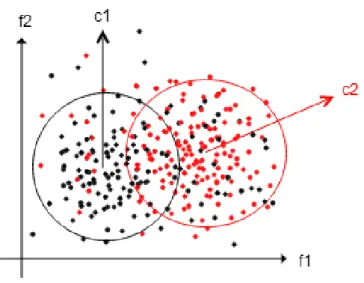
In K-Means Clustering method k cluster are determined and k sample are chosen as cluster centers, then by using Euclidean distance between each object and cluster center, instances are grouped according to closest center and cluster center recalculated. If the new cluster center is same with previous one, process ends, if not objects are grouped again and steps over. As an example of clustering you can see the Figure 3, instances have two features f1 and f2 and grouped into two cluster c1 and c2. Cluster centers are determined by using K-Mean clustering method and centers determined according to density of similar objects.

(23)

8

Figure 3: Unsupervised Learning/Clustering

We have four base collection or input sets. These are training dataset, training labels set, test dataset and test labels set. Because of having a label or a class set in our datasets, the method which we have used is supervised learning.

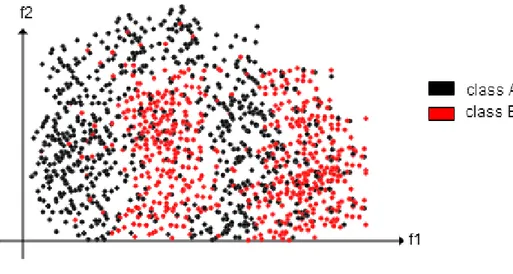
In supervised learning, a training algorithm is used with train data set and its class set. At the end of training part, the algorithm can be used to classify the data instance. When we apply a query from test dataset then the algorithm can make a guess what is the class of the test element. This prediction might be wrong or correct. We can compute the accuracy of the algorithm using test labels. Accuracy percentage of the algorithm depends on your algorithm and your training dataset. The dataset can contain fallacious information depending on missing or wrong value that decreases the accuracy of our classification and make the algorithm wrong guesses. Supervised learning has many different classification methods such as Decision trees, Naive Bayes, Random Forest and K-Nearest neighbor etc. In Figure 4, the collection of instances has two features as f1 and f2. Instances are grouped by their class information class A or B.

(24)

9

Figure 4: Supervised Learning/Classification

Supervised learning uses different model estimations to train and test the data set. These methods are Resubstitution Method, Hold-out Method, Leave one out Method and Rotation method.

1- ) Resubstitution Method: All the available data are used for training as well as for testing which means that the training and testing sets are the same. This method is preferred in real-world applications.

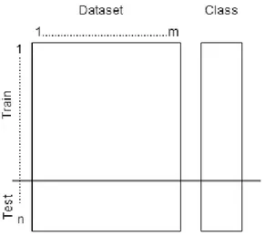
2- ) Hold-out Method: Half of the data or two-third of the data is used for training and the remaining data for testing as seen in Figure 5. Training and testing sets independent and the error estimation is pessimistic.

(25)

10

Figure 5: Model Estimation

3- ) Leave one out Method: A model is created using (n-1) samples for training and testing on the one remaining sample. This is iterated n times with different training sets of size (n-1). This approach needs large computational, because n different set must be created and computed.

4- ) Rotation Method (K-fold cross validation): This approach is an agreement between holdout and leave one out methods. It divides the available samples into p disjoint subsets, where 1 ≤ p ≤ n, (p-1) subsets for training and the remaining subsets for testing. This is the most popular method in practice. We create same number of model with the fold number as seen in Figure 6.

(26)

11

Figure 6: K-fold cross-validation

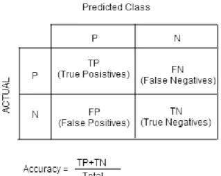
Assume that we have two classes in terms of positive samples versus negative samples. After training dataset, we measure how much the method learn this set and how much of test samples’ classification are guessed correctly. The ratio of correct classified samples over total classification gives the accuracy of out classification method (see Figure 7).

(27)

12 4.2 Methods

In this study, LSH and RF algorithms are considered. LSH is produced from K-NN so it is necessary to identify K-NN algorithm first. LSH and RF algorithms are also described in the following sections.

4.2.1 K-Nearest Neighbors Method

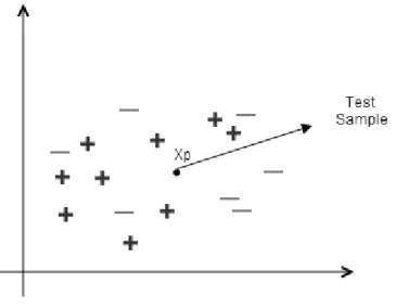
One of the most famous solution methods for the classification problem is finding the nearest neighbors of a specific query element. This method is also known as K-NN. K-Nearest Neighbors method was described by T. M. Cover and P. E. Hart in 1967. In this method, a distance metric can be defined such as Euclidean, cosine, hamming or Levenshtein. In the set of negatives and positives we consider the nearest neighbors in terms of distance metric which we use. See the Figure 8 in Euclidean space.

(28)

13

Indyk et al. [1] gives a definition of that method: Let T be a set of point for training data and assume that its size is n. We can denote T as T = { }. We need to specify a metric space and let S be our metric space. We can define a distance function df in our metric space S. Each element of T has got a class related to df in the metric space S. K-NN algorithm as pseudo code, can be given as follows:

Name: K-NN

Data: q is the query element, T is the training set, L is the training label set, n is size of the training set, k is the number of neighbors

Result: label of q initialization; distanceList ← ∅; for i ← 1 to n do t ← ; distanceList[i]←df(q, t); end for sortedElementsIncOrder ← sort(distanceList); labelCount ← {∅}; for i ← 1 to k do l ← L[index(sortedIncOrder[i])];

(29)

14

labelCount[l] ← labelCount[l] + 1;

end for

sortedLabels ← sortDecOrder(labelCount);

return sortedLabels[0];

Pseudo code 1: K-NN Algorithm

As shown as pseudo code of K-NN, the algorithm uses a distance function df. If our metric space S is Euclidean space, df can be defined as follows:

df =

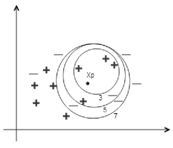
The K-NN algorithm calculates distance between query point and each training element using df function, and each distance is stored into distanceList. In the second step of the algorithm, all elements in the distanceList are sorted in increasing order according to their distances from q. After this step, the labels of the first k elements of the sortedElementsIncOrder are counted and counts of labels for the first k elements are stored in the labelCount map. In the last step of the K-NN algorithm, the labelCount map is sorted in a decreasing order as sortedLabels and the algorithm returns the first element of the sortedLabels. Actually the algorithm draws an imaginary circle around q which covers nearest neighbors (See Figure 9). K-NN algorithm is a brute force algorithm and it works in a reasonable time for small datasets. Thus it is not efficient for high dimensional and big datasets.

(30)

15

Figure 9: K-NN in Euclidean Space 4.2.2 Locality Sensitive Hashing (LSH) Method

Locality Sensitive Hashing finds the nearest neighbors in sublinear time. A function which runs in linear time needs to perform operations as its input size. In contrast to sublinear time, the function performs operations as less than its input size and functions which run in sublinear time grow slower than the functions which run in linear time for sufficient large input size. When LSH and NN are compared, K-NN needs to operate N operations for the dataset whose size is N but LSH can perform operations less than N for the same dataset.

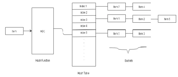
LSH is a learning algorithm which is based on hashing mechanism. Generally, hashing is common and very useful method in computer science. However hashing mechanism of LSH is different from general hashing. In general hashing methods have three parts: a hash function, a hash table and bucket(s). A hash function tries to generate unique integer or index value for a vector. For example, let w be a 1xd vector and it is sent to the hash function as a parameter, then the hash function

(31)

16

generates an integer for the vector w. A general hash function can be described as follows for vector w:

Let P be nine or ten digit prime number and ∈ Z Let T be an integer

h(w) = ( ( * + … + ) mod P ) mod T

However, generating a unique integer or index is impossible in every time. This case is called as collision. To overcome this problem, there is an associative data structure for hashing. This data structure called as hash table. Hash tables can be described as a contiguous memory block as an array and it contains a linked list at each index and these lists are called as buckets. When a collision occurs for a data element, the data element is stored into the linked list in generated index (See Figure 10).

(32)

17

LSH is separated into two parts: training and querying. For the training part, the similar elements are grouped into buckets in hash tables using a bunch of hash functions. In LSH, a hash function can be defined as follows for a data element t (it is assumed to be 1xd vector) in the training dataset:

Let P is nine or ten digit Prime number and ∈ is the finite set of prime numbers

Let M be number of hash tables

h(t) = ( ( * + … + ) mod P ) mod M

Format of each hash function in the function list is as function h(t). This function list is called as hash function family. A hash function family HF is defined as follows in LSH [1]:

Let df be the distance measure and and be two distance value according to df. We can define sensitivity parameters such as ( , , , ) and for every h in HF: if df(x, y) ≤ , then the probability h(x) = h(y) is at least .

if df(x, y) ≥ , then the probability h(x) = h(y) is at most . if > and < then Sim is a dissimilarity measure. if > and > then Sim is a similarity measure.

These functions are selected from the hash functions list randomly. Each element in training dataset is indexed by selected hash function and inserted into a bucket which is placed in that index. Indyk et al. [1] describes LSH such as pseudo code:

(33)

18 Name: LSH_Training

Data: T is the training dataset, L is the training label set, l is number of hash tables Result: Hash tables trained with T

H ← { , , …, }; //hash function family

B ← { , , …, }; //hash tables

foreach p in T do

← choose randomly from H; foreach table in B do hashIndex ← ; [hashIndex] ← p; end foreach end foreach return B;

Pseudo code 2: LSH Training Part Algorithm Name: LSH_Query

Data: q is a query point

candidates ← ∅;

foreach table in B do

← get from H;

(34)

19

append [hashIndex] to candidates;

end foreach

K ← k ;//constant number

label ← K-NN(q, candidates, K); // K-NN uses Euclidean distance in this implementation for df function.

return label;

Pseudo code 3: LSH Query Part Algorithm

LSH makes a bunch of buckets which contain similar data elements. For example, when two similar or equal class objects are hashed with randomly chosen hash functions they are in the same bucket with high probability. Then we can apply K-NN method to a much smaller dataset than the original dataset. If we compare LSH to general hashing methods, we can observe basic principles of LSH.

(35)

20

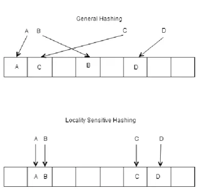
Figure 11: LSH vs. General Hashing Principle

In general hashing methods all items can be randomly placed to any indexes despite of their similarity (See Figure 11). In contrast to LSH, an index refers to a bucket or list of items which contain similar items with high probability. A randomly chosen hash function is responsible to generate these indexes according to similarity of items. That means all training data elements are inserted to the buckets with related to indexes. Thus, at the end of the training part we have got subsets of the original train dataset as many as number of hash tables.

When a query item comes from a test dataset, candidates are found for each table via hashing query item. The bucket which contains possible candidates is found using this index at O(1) time complexity. This is the power of all hashing methods. Now LSH algorithm knows that the query item belongs to a group of items. However it is not enough to classify the query data. Although all items in the same group are

(36)

21

assumed to be similar to each other, their classes or labels can be different. To classify the query element, we can apply the K-NN algorithm to that candidate set which contains similar items with the query point with a high probability in sublinear time. In big datasets, sublinear search performance has got a very important role. At the same time LSH algorithm can be considered as an algorithm to reduce dimension of dataset.

4.2.3 Random Forest (RF) Method

Decision trees are well known methods in machine learning and data mining. We can use decision trees to classify any object or data point. The most important issue for solving a classification problem using a decision tree is the construction of the correct tree. In contrast to decision tree method, Brieman et al. [2] described a new method which was named random forest (RF). RF is an ensemble technique in machine learning and it is very useful for categorical datasets. In RF, there is a bunch of decision trees which create a forest structure. Each decision tree in the forest has got a maximum depth and nodes which contain split features. Let N be the feature number of each data sample in our dataset and maximum split feature for each tree in the forest should be .

In training part of RF, each split features is picked from a random subset of the features. Instead of using the most discriminative thresholds, a random subset of features is used. Because of this randomness, the bias of the forest increases. RF has got an essential method for maintains accuracy when a large amount of data are missing and RF does not need to cross validation because it uses the out of bag error estimation. In the out of bag error estimation method, one out of three of the training dataset is dedicated for testing for created estimators or trees. After creating trees, each tree is tested with samples which are not in the tree and an error rate is estimated for each tree. The out of bag error estimation has proven to be unbiased. In

(37)

22

RF, each tree can enlarge as much as possible because RF does not prune any tree in the forest.

Information gain is the most important part of RF. We need to determine the best split for sub trees according to information gain calculation. Thus we calculate information gain for each leaf before splitting. Each leaf contains the result of classification, so we use entropy based calculation for each leaf and split to calculate information gain. Entropy can be given as follow:

entropy =

We used these four methods to construct a random forest following as: function constructTree(T, L, mD, mSF)

function split(leaf l, L)

function bestSplit(leaf l)

function informationGain(leaf l, split sp)

T is the train dataset, L is the train label set, mD is the maximum depth parameter, mSF is the number of maximum split features. We can define constructTree method

in a pseudo code format such that:

Name: constructTree

Data: T is the training set, L is the label list, mD is the maximum depth, mSF is the number of maximum split feature

(38)

23 if root is NULL do

S ← sample from T;

choose features SF randomly len(S) ≤ mSF; make a node N from SF ;

root ← N; end if

while depth of tree ≤ mD do

foreach sample s in T - S do

choose features SF randomly len(s) ≤ mSF; make a node l from SF

l’, l’’ ← split(l, L);

if l’ is left node do

attach l’ to left node of root;

end if

if l’’ is right node do

attach l’’ to right node of root;

end if end foreach end while

return root;

(39)

24 Name: split

Data: node l, set of label L

Result: left and right node with appropriate label BS ← bestSplit(l); if BS ≠ ∅ do lc ← makeLeftChild(l, L for BS); rc ← ∅; else rc ← makeLeftChild(l, L for BS); lc ← ∅; end if return lc, rc;

Pseudo code 5: Split Algorithm

Name: bestSplit Data: node l

BS ← ∅

for b ∈ possible splits for l do

(40)

25 if isValidSplit(l, b) do BS ← b; end if end if end for return BS;

Pseudo code 6: Best Split Algorithm Name: informationGain

Data: node l, split sp

lc ← makeLeftChildren(sp); rc ← makeRightChildren(sp);

return entropy(L[sp], l) – entropy(L[sp], lc) – entropy(L[sp], rc);

Pseudo code 7: Information Gain Algorithm

As shown as pseudo code for creating a decision tree, a split feature is selected randomly for each sample in the training dataset. The constructTree algorithm has got a criterion to halt the execution. If the tree has reached the maximum depth, it means that leaves have been constructed. Thus the algorithm is halted; otherwise a new node is created and the best split is calculated for the created node. The split function tries to find the best split for the node using bestSplit function. The bestSplit function calculates a best split score for the node with the current sub split feature set using informationGain function. In the informationGain function, an information gain is calculated creating possible right and left child node with a based on the

(41)

26

entropy calculation. At the end of the constructTree, a decision tree has been created dynamically.

Name: randomForest

Data: N is the number of tree, mD is the maximum depth for each tree, mSF is the number of maximum split feature, T is the training dataset, L is the training label set

oobTestData ← T;// one out of three of T training dataset is dedicated for

calculation of out of bag error

oobTestLabels ← L; // one out of three of L training label set is dedicated for

calculation of out of bag error treeList ←∅; for i ← 1 to N do t = constructTree( ); append t to treeList; end for weightedTreeList ← ∅;

foreach tree in treeList do

rate = calculate the out of bag error rate for tree using oobTestData and oobTestLabels;

if rate < do // = 0.37

increase the weight of tree for voting;

else

(42)

27 end if

append tree to weightedTreeList;

end foreach

forest ← combine trees from weightedTreeList;

return forest;

Pseudo code 8: Random Forest Algorithm

In the above pseudo code, one out of three of the training dataset T and one out of three of training label set L are used for calculating the out of bag(OOB) error rate for each tree which has been constructed with two out of three of T and L. If a tree has got an OOB error rate which is less than 0.37, weight of tree is increased for voting. After this step, all trees are combined as a forest and the algorithm returns the forest. Creating decision trees and a random forest classifier is the training part of the algorithm.

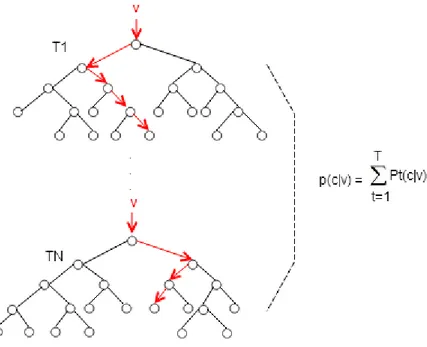
After creating the random forest classifier, we can ask class of an unknown element to the classifier. This part is called as querying. In the querying part, a query element in test dataset is classified by all trees in the forest. Then partial results are collected from all trees and top rated class is assigned to the query part. In addition to this, each tree returns the result class with a probability. When the votes for classes are equal, the classifier considers votes and probabilities for the query point q. Thus the classifier assigns the result class to the query point q according to its total votes and probabilities from all trees (See Figure 12).

(43)

28

Figure 12: Querying in Random Forest 4.3 Similarities between LSH and RF

In this unit, we talk about some similarities between LSH and RF algorithms. First of all two algorithms are related to classification problem. Thus both of them are supervised learning algorithm. Supervised learning means that an algorithm knows classes of each train data element before querying. The algorithm infers the class of a query element from previous knowledge which learned in the train part. In supervised learning, the algorithm creates a model (probabilistic or statistical) then in the query part, it uses this model to guess class of any data point. For example, when we ask an unknown data element to RF, RF algorithm creates forest as a model which contains class information and probabilities in leaves of each tree. After creating a model, the unknown element is searched in each tree in the forest and each tree returns a class and a probability for the unknown element. At the end

(44)

29

of the query part, RF determines the class of the query element according to numbers of classes which are collected from all trees in the forest if the numbers of classes are not equal, if they are equal then RF determines the class of the point according to the maximum probability of returned classes. Likewise, LSH also creates a model from train dataset. Hash table are probabilistic model for LSH. All data in the train dataset are inserted to hash tables which contain similar items with high probability. In query part of LSH algorithm, the algorithm tries to make a class guess for the query element using this hash tables. It applies K-NN to appropriate hash table for the unknown element.

The other similar characteristic of both algorithms is randomness. LSH and RF are randomized algorithms. LSH chooses a hash function from the hash function families or lists randomly. RF constructs all trees using random feature subsets from train dataset instead of a specific discriminative threshold value. These algorithms use randomness in their training part.

4.4 Implementation

We give a brief description about the implementation of core algorithms and some utility scripts for preparing datasets without going to details. We divided the implementation into two parts: implementation RF and LSH as core algorithms, implementation of data preprocessing scripts. In this section, some important points are mentioned to explain the reasons of choosing programming languages and third party tools.

4.4.1 Implementation of Core Algorithms

We implemented LSH and RF using Python programming language. Python is a scripting language and it is the most popular tools with MATLAB and R among data

(45)

30

scientists. Also many contributors develop numerous libraries for Python and one of them is Numpy(NP) [18]. We used standard Python library and NP array library. NP is an effective array library for Python. In Python, there is no C based array implementation. Instead of using contiguous memory blocks as an array in Python, we need to use a linked list implementation or primitive list data structure of Python. List data structure is not efficient enough for big datasets. Thus we preferred to use a C based array implementation for Python. NP is the most popular and the defacto standard in Python communities. NP has got also C based array structure and functions. Many benchmarks which are performed by NP developers show that NP is faster than primitive list data structure in standard Python library.

During the implementation time, we needed to perform some basic vector and matrix operations. These mathematical operators are implemented as an operator using operator overloading or a method in NP. It provides a clear interface to us for complex mathematical expressions when we implemented both two algorithms. The other third part library is Scikitlearn [19]. Scikitlearn has got many data mining algorithms. It also uses NP and dictionary data structures in Python. We used Scikitlearn for testing our RF implementation.

4.4.2 Implementation of Data Preprocessing Scripts

Another useful programming tool which we used data preprocessing is MATLAB. We created CSV files from MNIST and NOTMNIST datasets using MATLAB scripts. MNIST dataset has got a special file format to read all training and test datasets with their classes and the creator of MNIST dataset provides some third party MATLAB libraries to us. However, NOTMNIST dataset is a set of raw images. Thus we read all images and converted it to MAT objects. Finally we wrote

(46)

31

some utility functions to prepare training and test datasets for NOTMNIST in MATLAB.

(47)

32

Chapter 5 Experimental Results

In this section, experiment results are discussed. We examined the performance results of RF and LSH in terms of accuracy and running time for two different datasets. Results were calculated for 5000 and 10000 query or test elements. Moreover, both algorithms were trained with 60000 training data elements for both datasets.

LSH have got a sensitive parameter is called as number of tree, so this parameter was changed for all experiments. Although RF has got three different parameters, only one parameter was used in experiments. RF can be used for classification or regression. If RF is used for classification, maximum split feature parameter should be square root of the feature size. Thus the maximum split feature parameter was fixed for all experiments, so its value was equal to 28. The second fixed parameter of RF is maximum depth. This parameter was equal to 21, because RF reached a saturation point for accuracy when maximum depth was equal to 21. When it was changed, the accuracy did not change very much in our experiments.

Number of hash tables and number of estimators (trees) were chosen as equal. These values were 12, 16, 20, 24, 28 and 32. Performance of RF and LSH was measured with these values. In addition to these, resubstitution model was performed on RF and LSH using both datasets. Each performance experiment was performed 30 times for each number of hash tables and number of trees value. This is not a magic number. This value comes from the central limit theorem. According to this theorem, if the number of sample is greater than or equal to 30,

(48)

33

this sample size is sufficient to get approximate normal distribution for the distribution of the sample mean. Thus each experiment was tested 30 times. Processing and Analyzing Performance Results

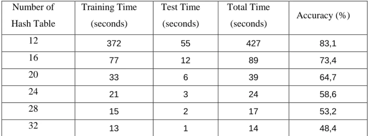
First of all, accuracy vs. execution time performance results of LSH for MNIST and NOTMNIST 5000 are shown in Table [1] and Table [2].

Number of Hash Table Training Time (seconds) Test Time (seconds) Total Time (seconds) Accuracy (%) 12 ₃₇₂ ₅₅ ₄₂₇ _83,1 16 ₇₇ ₁₂ ₈₉ _73,4 20 ₃₃ ₆ ₃₉ _64,7 24 ₂₁ ₃ ₂₄ _58,6 28 ₁₅ ₂ ₁₇ _53,2 32 ₁₃ ₁ ₁₄ _48,4

Table 1: LSH Running Time – Accuracy for 5000 MNIST Test Elements Number of Hash Table Training Time (seconds) Test Time (seconds) Total Time (seconds) Accuracy (%) 12 ₂₈₀ ₁₀₇ ₃₈₇ _81,2 16 ₁₄₀ ₃₀ ₁₇₀ _76,1 20 ₇₂ ₁₇ ₈₉ _70,4 24 ₄₈ ₉ ₅₇ _61,3 28 ₂₆ ₄ ₃₀ _54,7 32 ₂₂ ₂ ₂₄ _46,5

(49)

34 Number of Hash Table Training Time (seconds) Test Time (seconds) Total Time (seconds) Accuracy (%) 12 ₇₁₁ ₁₃₂ ₈₄₃ _92,8 16 ₁₂₈ ₁₇ ₁₄₆ _81,6 20 ₅₉ ₁₀ ₆₉ _73,5 24 ₃₅ ₆ ₄₁ _66,8 28 ₂₈ ₄ ₃₂ _61,2 32 ₂₅ ₃ ₂₈ _55,5

Table 3: LSH Running Time – Accuracy for 10000 MNIST Test Elements Number of Hash Table Training Time (seconds) Test Time (seconds) Total Time (seconds) Accuracy (%) 12 ₇₇₅ ₁₀₀ ₈₇₅ _90,7 16 ₃₅₁ ₂₄ ₃₇₅ _83,8 20 ₁₄₆ ₁₂ ₁₅₈ _70,3 24 ₅₉ ₇ ₆₆ ₆₃ 28 ₂₈ ₅ ₃₃ _56,1 32 ₂₄ ₄ ₂₈ _48,6

(50)

35

Figure 13: LSH MNIST – NOT MNIST 5000 & 10000 Accuracy – Execution Time

When the accuracy is maximum, the number of hash tables parameter of LSH is the minimum value for both datasets. For instance, when the number of hash

tables = 12, the accuracy of LSH equals to 83.1% and 81.2% for 5000 test

elements in Table [1] [2]. On the other hand, when the number of hash tables = 32, the accuracy of LSH equals to 48.4 and 46.5. It is below 50 percent. For 10000 query elements in Table [3] [4], this is true. Although the accuracy is decreasing, training, test and total execution time are decreasing with increase of number of hash tables. LSH returns the classification results for 10000 in 3 and 4 seconds. LSH behaves totally like K-NN for small number of hash tables, so the running time complexity of LSH converges to complexity of K-NN for a small number of hash tables and its accuracy is growing, in other words, LSH performs K-NN for a

(51)

36

set which contains more similar items. If the number of hash tables increases, each table contains less similar items. Thus LSH accuracy is decreasing and its execution time is decreasing, because each subgroup size is less than the original dataset size (See Figure 13).

Secondly, RF performances are shown in Table [5] [6] [7] [8] for MNIST-NOTMNIST 5000 and MNIST-MNIST-NOTMNIST 10000.

Number of Tree Training Time (seconds) Test Time (seconds) Total Time (seconds) Accuracy (%) 12 ₅₈ ₂ ₆₀ ₈₇ 16 ₇₂ ₃ ₇₅ _87,2 20 ₉₀ ₄ ₉₄ _87,4 24 ₁₀₂ ₄ ₁₀₆ _87,6 28 ₁₂₆ ₅ ₁₃₁ _87,7 32 ₁₅₂ ₅ ₁₅₇ _87,7

Table 5: RF Running Time – Accuracy for 5000 MNIST Test Elements Number of Tree Training Time (seconds) Test Time (seconds) Total Time (seconds) Accuracy (%) 12 ₁₀₃ ₅ ₁₀₈ _82,7 16 ₁₃₂ ₅ ₁₃₂ _83,2 20 ₁₅₄ ₇ ₁₅₄ _83,6 24 ₁₈₆ ₈ ₁₉₄ _83,8 28 ₂₃₅ ₁₀ ₂₄₅ _84,1 32 ₂₇₆ ₁₂ ₂₈₈ _84,2

(52)

37 Number of Tree Training Time (seconds) Test Time (seconds) Total Time (seconds) Accuracy (%) 12 ₁₀₁ ₃ ₁₀₄ _93,1 16 ₁₃₄ ₆ ₁₄₀ _93,6 20 ₁₆₆ ₆ ₁₇₂ _93,8 24 ₁₉₉ ₇ ₂₀₆ _93,8 28 ₂₃₅ ₈ ₂₄₃ _93,9 32 ₂₆₉ ₉ ₂₇₈ _93,9

Table 7: RF Running Time – Accuracy for 10000 MNIST Test Elements Number of Tree Training Time (seconds) Test Time (seconds) Total Time (seconds) Accuracy (%) 12 ₁₃₉ ₇ ₁₄₆ _90,1 16 ₁₈₉ ₉ ₁₉₈ _90,8 20 ₂₄₆ ₁₃ ₂₅₉ _91,2 24 ₂₉₄ ₁₇ ₃₁₁ _91,4 28 ₃₃₂ ₂₀ ₃₅₂ _91,4 32 ₃₇₅ ₂₆ ₄₀₁ _91,5

(53)

38

Figure 14: RF MNIST – NOT MNIST 5000 & 10000 Accuracy – Execution Time Accuracy of RF is increasing when the number of trees is increasing, because the forest converges to be unbiased. However, training and testing time are increasing. For example, RF accuracy, training and testing time are increasing when the number of trees increases from 24 to 28 in Table [5] [6] [7] [8]. Though its accuracy is increasing, the increment goes to a limit or saturation point as seen in Figure 14. The reason of increment in the training and testing time is that RF creates much more decision trees in the training part and a test element is classified by each tree in the forest in the testing part.

(54)

39

Figure 15: LSH- Training Performance for MNIST

(55)

40

Figure 17: RF- Training Performance for MNIST

(56)

41

When RF and LSH algorithms are compared with each other in terms of accuracy and execution time, some critical points occurs. For example, LSH is not fast as RF if accuracy of LSH is maximum value for both datasets (See Figure 13 and Figure 14). When LSH is faster than RF for number of table = 32, accuracy of the RF is greater than LSH as seen in Table [4] and Table [8].

Resubstitution model is applied to these two algorithms using MNIST and NOTMNIST datasets. RF and LSH are trained with MNIST and NOTMNIST 60000 and for the test part, number of hash tables and number of tree parameters are 30, 32, 34 and 38. This model shows that two algorithms are over trained. Accuracies of these algorithms are greater than 99% (Figure 15, 16, 17, 18). This case is called as overfitting in machine learning and data mining. Some learning algorithms can be affected negatively by overfitting and some algorithm cannot be affected, but LSH is affected. LSH learns every data items in the training dataset perfectly. When a new test element comes from test dataset, LSH cannot classify this query element correctly. One of the reasons of having less accuracy for LSH can be overfitting.

(57)

42

Chapter 6 Conclusion

In this thesis, we implemented two popular machine learning algorithms with their various parameters. After that we run these two algorithms on public datasets which are called MNIST and NOTMNIST. Our goal is that creating a main idea observing the pros and cons of these two algorithms to develop a new hybrid algorithm in the future. The datasets we worked on are myriads of digitized images digits and characters.

The scope of the thesis after observing mechanism of these two algorithms, a literature research has been done in-depth looking existing studies. In this research direction, we learned that there were practical applications of existing two classification algorithms RF and LSH in some important research areas such as image processing, pattern recognition and bioinformatics. We run these algorithms on the datasets which we mentioned in previous paragraph after implementing two algorithms using Python programming language in Linux environment. We did not encounter any problem during the running time of our application. We examined the results which were generated by our work in details in the related section. According to these results, our highlighted impressions are that both of two algorithms are successful in their using areas.

LSH algorithm is an approach which creates specific amount of subsets from the original dataset for big datasets. As a result of our experiments, we checked accuracy and running time of this algorithm via changing its number of hash table parameter. When we reached the optimal parameters of LSH, we observed that LSH was running faster than RF but was not successful to classify like RF in

(58)

43

terms of accuracy. As we mentioned before LSH was designed for big datasets so it was very fast but it was not accurate.

RF algorithm is a forest which contains many decision trees. As a supervised classification algorithm RF is more successful than LSH which is a hashing method in terms of accuracy. In order to that, it is running fast as LSH. On the contrary, we observed some cases that RF is slower than LSH because RF requires much more memory than LSH.

Finally, our belief became much stronger to create a hybrid algorithm which would be more accurate and faster combining both two algorithms in this work which we observed the pros and cons of these two algorithms. Moreover, we have another idea that determining automatically optimal parameters of these two parameter sensitive algorithms in the future.

(59)

44

References

[1] P. Indyk and R. Motwani, “Approximate nearest neighbors: Towards removing the curse of dimensionality,” in The 30th Annual ACM Symposium on Theory of Computing, 1998, p. 604.

[2] L. Breiman, “Random forests,” Machine Learning, vol. 45, no. 1, pp. 5–32, 2001.

[3] Y. Lin and Y. Jeon, “Random forests and adaptive nearest neighbors,” University of Wisconsin, Tech. Rep. 1055, 2002.

[4] Z. Yang, W. T. Ooi, and Q. Sun, “Hierarchical, non-uniform locality sensitive hashing and its application to video identification,” in IEEE International Conference on Multimedia and Expo (ICME), 2004, pp. 743–746.

[5] M. Datar, N. Immorlica, P. Indyk, and V. S. Mirrokni, “Locality-sensitive hashing scheme based on p-stable distributions,” in Proceedings of the 12th Annual Symposium on Computational Geometry, 2004, pp. 253–262.

[6] K. Terasawa and Y. Tanaka, “Locality sensitive pseudo-code for document images,” in The 9th International Conference on Document Analysis and Recognition (ICDAR), 2007, pp. 73–77.

[7] Y. Hua, B. Xiao, D. Feng, and B. Yu, “Bounded LSH for similarity search in peer-to-peer file systems,” in International Conference on Parallel Processing, 2008, pp. 644–651.

[8] Q. Wang, Z. Guo, G. Liu, and J. Guo, “Entropy based locality sensitive hashing,” in International Conference on Acoustics, Speech, and Signal Processing (ICASSP), 2012, pp. 1045–1048.

[9] S. Bernard, S. Adam, and L. Heutte, “Using random forests for handwritten digit recognition,” in Proceedings of the 9th International Conference on Document Analysis and Recognition (ICDAR), 2007, pp. 1043–1047.

(60)

45

[10] Y. Lecun, L. Bottou, Y. Bengio, and P. Haffner, “Gradient-based learning applied to document recognition,” in Proceedings of the IEEE, 1998, pp. 2278– 2324.

[11] S. Bernard, L. Heutte, and S. Adam, “On the selection of decision trees in random forests,” in International Joint Conference on Neural Networks (IJCNN), 2009, pp. 302–307.

[12] R. Caruana, N. Karampatziakis, and A. Yessenalina, “An empirical evaluation of supervised learning in high dimensions,” in International Conference on Machine Learning (ICML), 2008, pp. 96–103.

[13] S. Li, E. Harner, and D. Adjeroh, “Random knn feature selection - a fast and stable alternative to random forests,” BMC Bioinformatics, vol. 12, p. 450, 2011. [14] M. Zahedi and S. Eslami, “Improvement of random forest classifier through localization of Persian handwritten ocr,” ACEEE International Journal on Information Technology, vol. 2, no. 1, pp. 13–17, 2012.

[15] Y. Mu, J. Sun, T. H. , L. Cheong, and S. Yan, “Randomized locality sensitive vocabularies for bag-of-features model,” in Proceedings of the 11th European Conference on Computer Vision (ECCV), Heraklion, Crete, Greece, 2010, pp. 748– 761.

[16] Y. LeCun, C. Cortes, and C. Burges, “THE MNIST DATABASE of handwritten digit,” http://yann.lecun.com/exdb/mnist/.

[17] Y. Bulatov, “notMNIST Dataset,” http://yaroslavvb.blogspot.com/2011/ 09/notmnist-dataset.html, 2011, [Online; accessed 25-September-2013].

[18] Numpy, “Numpy,” http://www.numpy.org/, 2013, [Online; accessed 25-September-2013].

[19]Scikit-Learn, “Random Forest,”

http://scikit-learn.org/stable/modules/ensemble.html#forest, 2010, [Online; accessed 25-September-2013].

(61)

46

Curriculum Vitae

Aykut Çayır was born in August 26th, 1988, in Istanbul. He received his BS in Computer Engineering in 2011 at Kadir Has University. From 2011 to 2013, he worked as a graduate assistant at Kadir Has University. He worked as a software engineer at AGMLab between June and September 2013. Now he is a data engineer at HemTeknoloji.